Review

Steel Surface Defect Recognition: A Survey

1
School of Software, Shenyang University of Technology, Shenyang 110870, China
2
School of Mechanical Engineering & Automation, Northeastern University, Shenyang 110819, China
*
Author to whom correspondence should be addressed.
Coatings 2023, 13(1), 17; https://doi.org/10.3390/coatings13010017
Submission received: 17 October 2022 / Revised: 2 December 2022 / Accepted: 4 December 2022 / Published: 22 December 2022
(This article belongs to the Special Issue Solid Surfaces, Defects and Detection)

Abstract

:
Steel surface defect recognition is an important part of industrial product surface defect detection, which has attracted more and more attention in recent years. In the development of steel surface defect recognition technology, there has been a development process from manual detection to automatic detection based on the traditional machine learning algorithm, and subsequently to automatic detection based on the deep learning algorithm. In this paper, we discuss the key hardware of steel surface defect detection systems and offer suggestions for related options; second, we present a literature review of the algorithms related to steel surface defect recognition, which includes traditional machine learning algorithms based on texture features and shape features as well as supervised, unsupervised, and weakly supervised deep learning algorithms (Incomplete supervision, inexact supervision, imprecise supervision). In addition, some common datasets and algorithm performance evaluation metrics in the field of steel surface defect recognition are summarized. Finally, we discuss the challenges of the current steel surface defect recognition algorithms and the corresponding solutions, and our future work focus is explained.

1. Introduction

Steel is one of the most common metal materials in our daily life, where its uses are numerous, and steel is the perfect material in many fields. Steel is widely used in civil engineering infrastructure, aerospace, shipbuilding, automotive, machinery manufacturing, and the manufacture of various household tools. According to the World Steel Association, the global steel demand is expected to continue to rise by 0.4% in 2022, with annual production reaching 1840.2 billion tons, more than all the other metals combined [1]. Today, steel is a key material for manufacturing, infrastructure, and other industries. Since the quality of steel will directly affect the quality of manufactured products and infrastructure construction, it is particularly important to control the quality of the steel produced, as this is the first guarantee of qualified products.
For the recognition of steel surface defects, it mainly includes three functions: detection, classification, and the location of defects. The detection of defects is to determine whether the inspection object contains defects; the classification of defects is, as the name implies, the classification of defect categories; and the location of defects is to determine the location of defects in the inspection object. The result of this defect location will be different for different algorithms; most algorithms display a rough anchor frame to locate the defect, while there are more accurate methods that can directly describe the shape of the defect down to the pixel level.
However, the recognition of defects on the steel surface is more difficult, and the main reasons why it is difficult to identify are as follows. First, there is an inter-class similarity and intra-class diversity of defects on the steel surface [2]. Second, there are many types of steel surface defects and some of these defects may overlap, while most classification tasks can only find the defects with the highest confidence level in the defect category, resulting in imprecise classification results [3]. In the actual production environment, it is very difficult to obtain high quality datasets for training machine learning related algorithms because defects in steel production are originally small probability events, and it is very difficult to obtain many samples with various types of defects; the labeling of the data is also costly and labor intensive [4,5,6,7]. Since the classification of defect categories is based on human subjective classification and there is still no strict classification standard, these lead to difficulties in the progress of classification work. In addition, in the actual production environment, the interference of the environment is serious such as uneven lighting, light reflection, noise, motion blur, the existence of many false defects, and a low contrast of background clutter, resulting in the recognition effect being often less than ideal [8]. Although the introduction of more image sensors (depth and thermal infrared) [9] can effectively reduce the influence of various interference factors, it also creates a lot of redundant information. The contradiction between accuracy and speed is also one of the main problems faced by the defect recognition algorithm [10]; in the actual production environment, the speed of the assembly line is relatively fast, for flat steel products, the assembly line running speed is about 20 m/s, for long wire, its product production assembly line running speed is up to 100 m/s. To achieve real-time detection, the algorithm developed must have a high enough accuracy at the same time, and the recognition speed is also fast enough. However, these two points are often contradictory in the design process of the algorithm. In the recognition of some small defects, it can be found that the defect area is too small in relation to the whole detection object, which leads to the detection object defect characteristics not being obvious. In addition, the manufacturing industry may be different for different steel mills, which may lead to different types of defects in their products, so the generalization of the algorithm will not be ideal, and it will be more difficult to produce a high-quality general dataset, which needs to go to different steel mills to collect samples. Finally, the collection of image samples of the inspected objects is also difficult, because for some steels, multiple planes need to be inspected, which leads to the need for multiple cameras to ensure complete coverage of the steel surface, so the collection of images from multiple cameras is also difficult.
The most common steel products include hot/cold rolled strip, bar/wire rod, slab, billet, and plate, which cover most of the uses of steel as a basic application material. The study of hot/cold rolled steel strips has received the most attention, mainly because most of these products are finished products. In terms of shape, the steel surface can be divided into flat products and long products [11]. Among them, flat products can be subdivided into slab/billet, steel plate, hot/cold rolled strip, and coated strip. Strip products include rods/wires, which are made by a hot rolling process with an oxidized surface, and other products such as rails, angle steel, channel steel, etc., which have a complex cross section, so the detection is also more complex. The specific division structure of the steel surface types is shown in Figure 1.
The existence of different defects on the surface of different types of steel and the absence of an accepted standard for the classification of defects leads to the possibility of a certain irrationality in the classification of defects, which adds to the difficulties in their recognition. In this paper, the defect categories mainly detected in a large amount of literature are summarized, and the defect catalog published by Verlag Stahleisen GmbH [12] was used as a basis to summarize the defect categories contained in the steel surface for the types of the steel surface, and the specific defect categories are shown in Table 1.
The steel surface defect recognition methods go through three stages: manual recognition, the traditional machine learning algorithm, and deep learning algorithm. The milestones regarding the development of industrial surface defect technology are shown in Figure 2.
The first stage of manual recognition methods refer to the detection of steel surface defects by quality inspectors, mainly by virtue of manual experience and subjective judgment: there are low efficiency, labor intensity, low precision, poor real-time, and other defects [34]. In addition, the human eye observation range and speed are limited, generally requiring that the product width cannot exceed 2 m and the product movement speed cannot exceed 30 m/s, otherwise the human eye will not be able to make effective observations [35], so manual defect recognition can no longer meet the increasingly developed industrial practical production environment. The second is the traditional machine learning algorithm, which generally needs to manually design the feature extraction rules of the recognition object, which is extremely dependent on the expert’s knowledge judgment, so human experience plays a decisive role in these methods, resulting in poor robustness of the algorithm and insufficient generalization ability. Traditional machine learning methods generally combine feature extraction methods with classifiers such as SVM to realize defect recognition. Such methods are usually sensitive to defect size and noise, and are generally not end-to-end models that cannot meet the needs of automatic defect recognition [36]. In addition, conventional machine learning methods rely on certain assumptions to be valid [37], for example, the color depth of the defective part is not the same as the background part, which limits the scope of application of this type of algorithm. For deep learning algorithms, with the advancement in computing power, they have gradually started to become popular in the field of surface defect detection in recent years, and deep learning methods have gradually been introduced into steel surface defect recognition. These methods can autonomously extract image features in the dataset through neural network models, and the characterization capability is more powerful, avoiding the manual design of feature extraction rules, which can effectively overcome the shortcomings of traditional machine learning methods. However, deep learning methods also have some challenges in the actual application environment, as described in Section 5.
The rest of this paper is organized as follows. In Section 2, the key elements of the hardware architecture of the steel surface defect detection system will be discussed. In Section 3, the steel surface defect recognition algorithms are classified and summarized. In Section 4, the datasets and algorithm performance evaluation metrics used in recent papers are summarized. In Section 5, the existing challenges of the steel surface defect recognition algorithm are described, and suggestions for their solution are provided. In Section 6, the entire paper is summarized, and the future directions of our work are described.

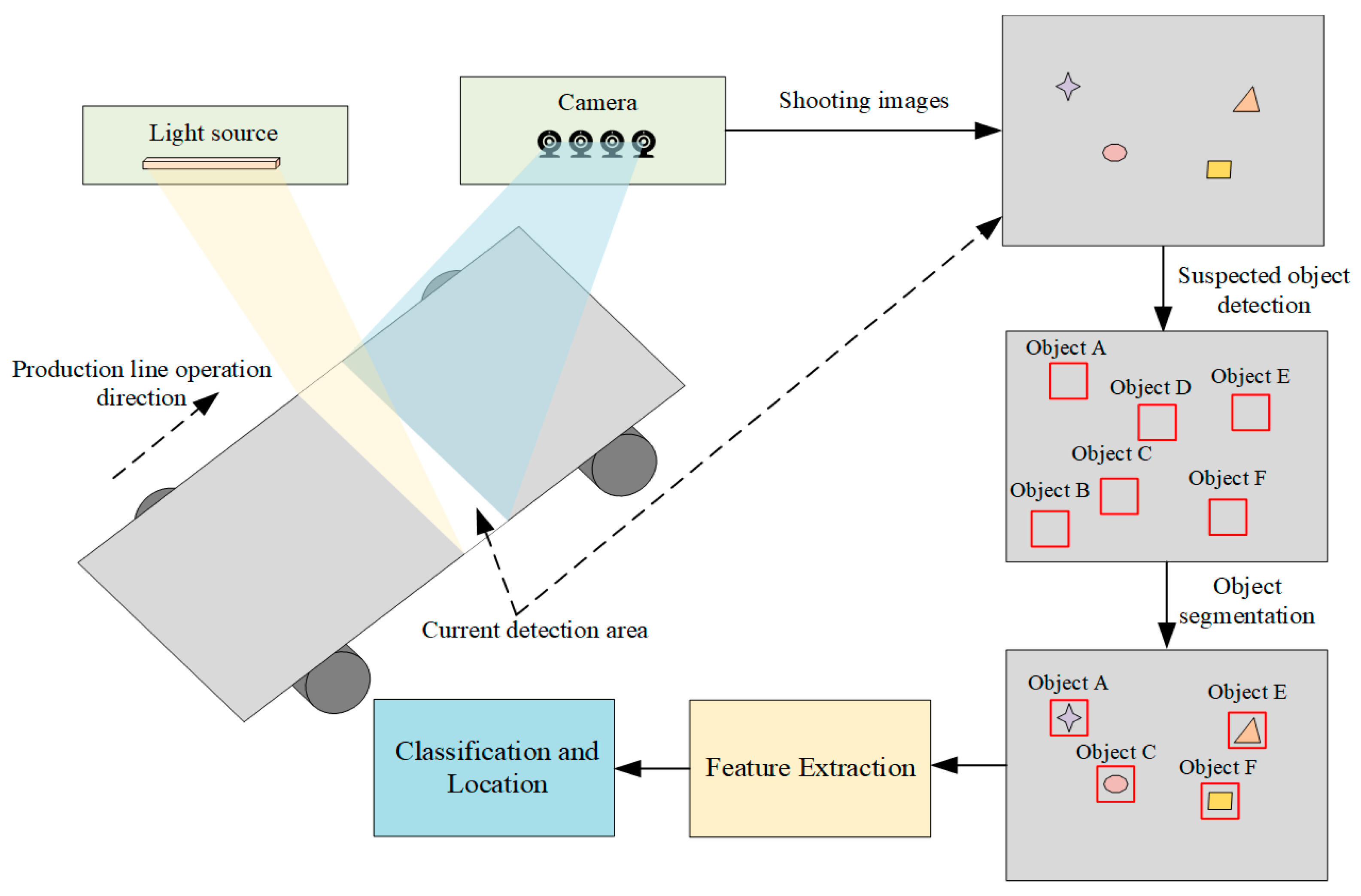
2. Key Hardware for Steel Surface Defect Recognition System

A complete steel surface defect recognition system consists of three parts: image acquisition, defect recognition, and quality control. The image acquisition aims to measure and capture the image information of the object to be inspected using an optical system that consists of a camera or analog camera and an illumination system. The camera is used to capture the image of the object to be detected, while the light source is used to assist the camera in capturing a higher quality image, which is beneficial for improving the detection accuracy and training efficiency. The defect recognition process is implemented by the software algorithm, and the specific description of the defect recognition algorithm is described in Section 3. The defect recognition section delivers the recognition results to the quality control section, thus displaying the strengths and weaknesses of the detected object as well as key information such as the type and location of the defect, etc. The quality control section only requires the reading and display of the information, so no detailed description is needed. A diagram of the steel surface defect recognition system is shown in Figure 3.

2.1. Camera

Industrial cameras can be classified according to the output mode and can be divided into two categories: analog cameras and digital cameras. As the output signal form of analog camera is a standard analog video signal, it needs to be equipped with a special image acquisition card to be converted into digital information that can be processed by a computer. Analog cameras are generally used in the field of TV cameras and surveillance, with the characteristics of good versatility and low cost, but generally lower resolution, slow acquisition speed, and the image transmission is susceptible to noise interference, resulting in image quality degradation, so it can only be used for machine vision systems with low requirements for image quality. In contrast, digital cameras are integrated with internal A/D conversion circuit, which can directly convert the analog image signal into digital information, which not only effectively avoids the problem of interference in the image transmission line, but also generates higher quality images. Compared with analog cameras, digital cameras also have higher resolution and frame rate, smaller size, and less power consumption requirements [38]. Therefore, digital cameras are more suitable for working in fast steel production lines and complex environments in real steel mills than analog cameras.
If divided by chip type, industrial cameras can be further divided into two categories: charge coupled device (CCD) cameras and complementary metal oxide semiconductor (CMOS) cameras. The difference between these two cameras lies in the way that light is converted into electrical signals. For CCD sensors, light striking the image element generates an electric charge that is transmitted and converted into the current, buffer, and signal output through a small number of output electrodes. For CMOS sensors, each image element completes its own charge-to-voltage conversion while generating digital signals. CCD cameras do not have an absolute advantage over CMOS cameras because CCD sensors can adapt to the brightness range of 0.1–3 lux, which is 3 to 10 times higher than the general CMOS cameras, so the current general CCD cameras have a higher imaging quality than CMOS cameras. However, because the CMOS sensor has a photosensitive element, amplifier, A/D converter, memory, digital signal processor, and computer interface control circuit integrated in a silicon chip, it has a simple structure, is fast, has a low power consumption, low cost, and other characteristics. With the development of technology, the CMOS camera’s poor image quality, small image sensitive unit size, and other problems have gradually been solved by the emergence of an “active image sensitive unit”, which increased the ability to resist noise. This means that CMOS sensors have an almost comparable sensitivity with CCD sensors, the image quality can be improved, and in terms of power consumption, the processing speed is better than that of CCD sensors. Therefore, many people believe that CMOS will become the leading sensor technology for machine vision in the future [39]. In light of the actual production environment in steel mills, CMOS cameras are more suitable for future defect detection systems. CMOS sensors do not require complex processing and directly convert the electrons generated by the image semiconductor into a voltage signal, so they are very fast, an advantage that makes CMOS sensors very useful for high frame cameras, where high frame speeds can easily reach over a thousand frames at speed, which is very suitable for high-speed production lines.
In summary, since the steel surface defect recognition process and the capture of dataset images are generally performed on steel mill production lines, and the actual steel mill needs to face the complex and harsh inspection environment of vibration, light, high temperature, fast, steam and oil, etc., CMOS type digital cameras are recommended as the actual image capture tool.

2.2. Light Source

As the camera exposure time is relatively short when shooting at high speed, in order to let enough light into the camera in a short time, proper fill light is essential. A suitable lighting system can help the camera capture sharper images, thus making the entire inspection system more efficient and accurate. Light sources often used in machine vision are fluorescent, incandescent, xenon, and light emitting diode (LED). Among them, the LED light source is the most widely used in the field of steel defect recognition [40,41,42]. This is because the LED lighting cycle is long, can generally be illuminated for up to 100,000 h, and with its lower heat, low power consumption, uniform and stable brightness, and variety of colors can be made into a variety of shapes and sizes and can set a variety of irradiation angles to meet a variety of lighting needs. In addition, the LED light source response is fast, can reach maximum brightness in 10 microseconds or less, has a power supply with an external trigger, can be controlled by computer, has fast start, low operating costs, and long life LED, which will reflect greater advantages in terms of the comprehensive cost and performance. Guidelines for setting up the LED light source can be found in [43]. Since some steel surfaces are relatively smooth, specular reflections need to be avoided as much as possible, so diffusers can be added to the light set to reduce the glare reflected from the metal samples.

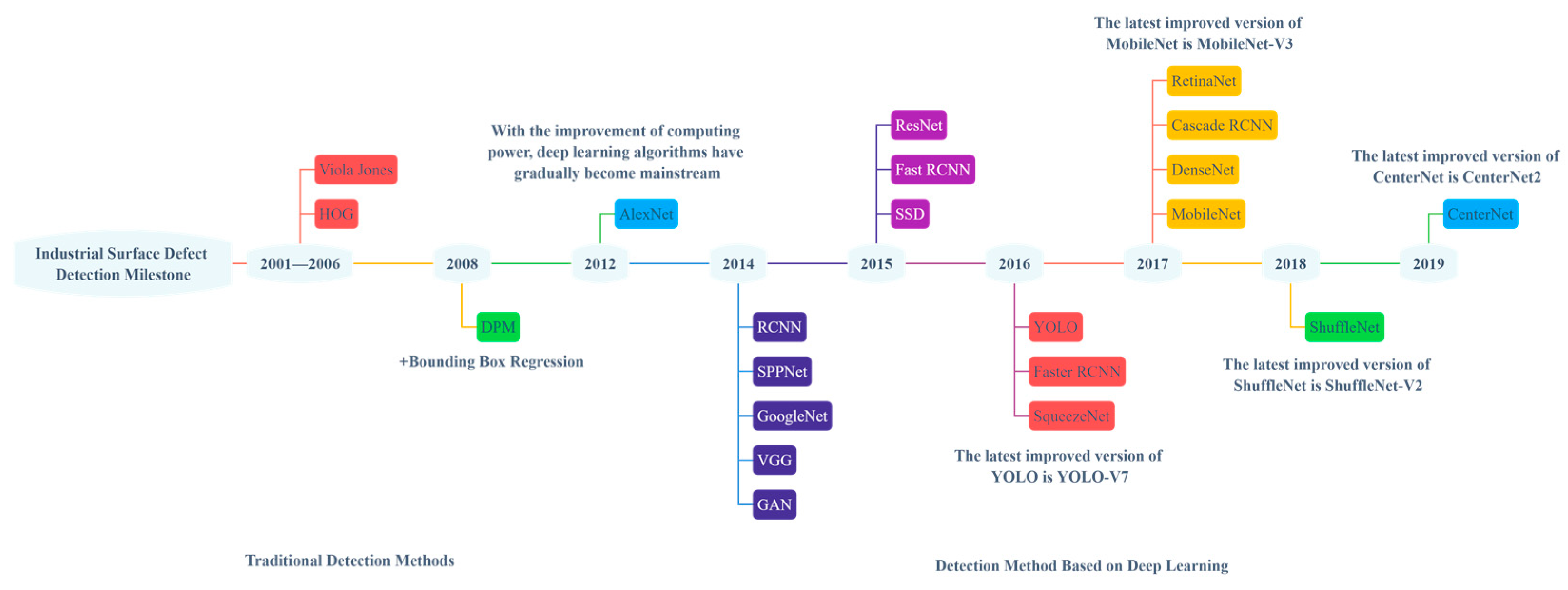
3. Algorithm Classification and Overview

Steel surface defect detection algorithms are classified according to whether deep learning techniques are applied and can be divided into traditional machine learning-based algorithms and deep learning-based algorithms. The traditional machine learning algorithms can be broadly classified into three categories: texture feature-based methods, color feature-based methods, and shape feature-based methods. The algorithms based on deep learning can be roughly divided into supervised methods, unsupervised methods, and weakly supervised methods. Of course, deep learning methods can also be classified according to the function of the selected neural network, which can be divided into image classification networks and object detection networks. Among them, image classification networks such as the classic AlexNet, ResNet, Visual geometry group (VGG), etc., and object detection networks can be divided into single-stage methods and two-stage methods, single-stage methods such as the well-known You only look once (YOLO) and Single shot multibox detector (SSD), and two-stage networks such as Fast R-CNN and Faster R-CNN.

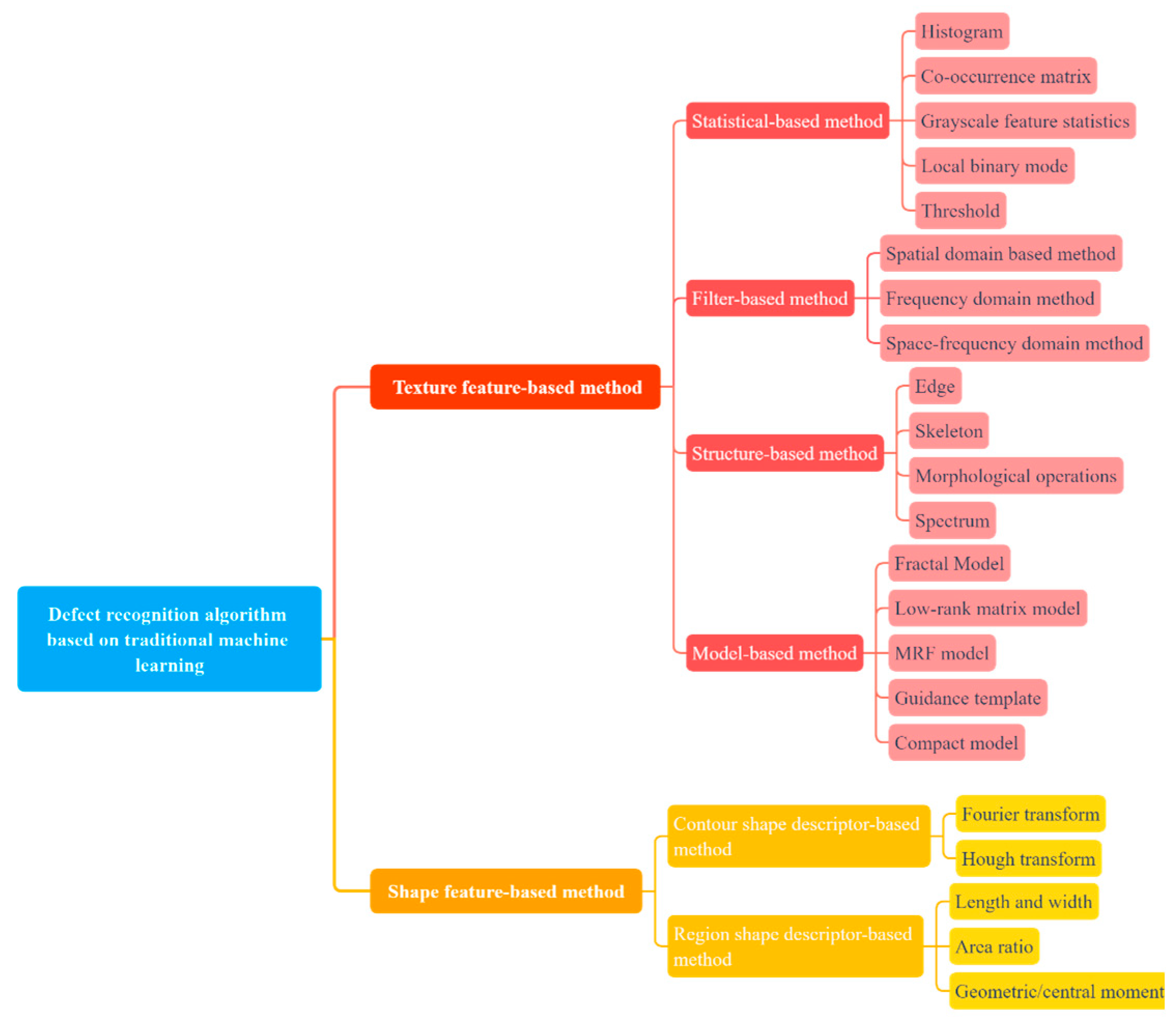
3.1. Defect Recognition Algorithm Based on Traditional Machine Learning

The traditional machine learning approach was an epoch-making advancement from manual inspection, and usually starts with the manual design of feature extraction rules, followed by feature extraction, and finally feeds the extracted features into the classifier to achieve the classification of defects. Because of the reliance on manually designed feature extraction rules, it leads to poor robustness and generalization ability of the algorithm and is susceptible to interference and the influence of noise, thus reducing the detection accuracy. The most traditional methods basically only provide a defect classification function and do not perform defect localization or segmentation, which is an incomplete defect recognition process. The machine learning algorithms used for steel surface defect recognition can be broadly classified into texture feature-based methods, shape feature-based methods, and color feature-based methods. However, in the field of steel surface defect detection, since color features mainly refer to grayscale features of the image, and the methods used to extract grayscale features are statistically based, the color feature-based methods were classified here under the texture feature-based methods. An illustration of the classification based on traditional machine learning methods in the field of steel surface defect recognition is shown in Figure 4.

3.1.1. Texture Feature-Based Methods

Texture feature-based methods are the most common methods in the field of steel defect detection, which reflects the homogeneity phenomenon in the image and can reflect the organization and arrangement characteristics of the image surface through the grayscale distribution of pixels and their nearby spatial neighborhood [44]. As shown in Figure 4, it can be subdivided into statistical-based methods, filter-based methods, structure-based methods, and model-based methods. These four methods can be used in combination or in conjunction with each other to achieve a higher performance. Regarding the literature on texture-based feature methods, these are shown in Table 2.
Statistical-based methods are used to measure the spatial distribution of pixel values, usually by using the grayscale distribution of image regions to describe texture features such as heterogeneity and directionality. Its common statistical methods include histogram, co-occurrence matrix, local binary patterns, etc. In 2015, Chu et al. [47] proposed a feature extraction method based on smoothed local binary patterns, which is insensitive to noise and invariant to scale, rotation, translation, and illumination, so the algorithm can maintain a high classification accuracy for the identification of strip surface defects. In 2017, Truong and Kim [48] proposed an automatic thresholding technique, which is an improved version of the Otsu method with an entropy weighting scheme that is able to detect very small defect areas. Luo et al. [49] proposed a selective local binary pattern descriptor, which was used to extract defect features, and then combined it with the nearest neighbor classifier (NNC) to classify strip surface defects; this algorithm pursued the comprehensive performance of recognition accuracy and recognition efficiency. The following year, Luo et al. [52] also proposed an improved generalized complete local binary pattern descriptor and two improved versions of the improved complete local binary pattern descriptor (ICLBP) and improved the complete noise-invariant local structure pattern (ICNLP) to obtain the surface defect features of the hot rolled steel strip, and then used the nearest neighbor classifier to achieve defect recognition classification, thus achieving high recognition accuracy. Zhao et al., in 2018 [51], designed a discriminative manifold regularized local descriptor algorithm to obtain steel surface defect features and complete matching by the manifold distance defined in the subspace to achieve the classification of defects in images. In 2019, Liu et al. [53] proposed an improved multi-block local binary pattern algorithm to extract the defect features and generate grayscale histogram vectors for steel plate surface defect recognition, and this work was able to recognize images at 63 FPS with a high detection accuracy at the same time.
Filter-based methods are also called spectrum based methods and can be divided into spatial domain based methods, frequency domain methods, and space–frequency domain methods. They aim to treat the image as a two-dimensional signal, and then analyze the image from the point of view of signal filter design. The filter-based methods include curvelet transform, Gabor filter, wavelet transform, and so on. Xu et al. [54] achieved the multiscale feature extraction of surface defects of a hot-rolled steel strip by curvilinear wave transform and kernel locality preserving projections (KLPP), thus generating high-dimensional feature vectors before dimensionality reduction, and finally, defect classification by SVM. In 2015, Xu et al. [55] designed a scheme that introduced Shearlet transform to provide effective multi-scale directional representation, where the metal surface image is decomposed into multiple directional sub bands by Shearlet transform, thus synthesizing high-dimensional feature vectors, which were used for classification after dimensionality reduction. Doo-chul CHOI et al. [57] used a Gabor filter combination to extract the candidate defects and preprocessed them with the double threshold method to detect whether there were pinhole defects on the steel plate surface. In 2018 [58], the classification of surface defects of a hot-rolled steel strip was achieved by extracting multidirectional shear wave features from the images and performing gray-level co-occurrence matrix (GLCM) calculations on the obtained features to obtain a high-dimensional feature set, before finally using principal component analysis (PCA) for dimensionality reduction followed by SVM for defect classification. Liu et al. [61] improved the contour wave transform based on the contour wave transform and the non-downsampled contour wave transform, and combined the multi-scale subspace of kernel spectral regression for feature extraction to achieve a relatively good recognition speed and the algorithm is applicable to a wide range of metallic materials.
The core goal of structure-based methods is to extract texture primitives, followed by the generalization of spatial placement rules or modeling, which is based on texture primitive theory. Texture primitive theory indicates that texture is composed of some minimal patterns (texture primitive) that appear repeatedly in space according to a certain rule. This method is applicable to textures with obvious structural properties such as texture primitives such as density, directionality, and scale size. In 2014, Song et al. [65] used saliency linear scanning to obtain oiled regions and then used morphological edge processing to remove oil interference edges as well as reflective pseudo-defect edges to enable the recognition of various defects in silicon steel. In 2016, Shi et al. [41] reduced the effect of interference noise on defect edge detection by improving the edge detection Sobel algorithm, thus achieving accurate and efficient localization of rail surface defects. Liu et al. [63] proposed an enhancement operator based on mathematical morphology (EOBMM), which effectively alleviated the influence of uneven illumination and enhanced the details of strip defect images. In 2016, [64] applied morphological operations to extract features of railway images and used Hough transform and image processing techniques to detect the track images obtained from the real-time camera to accurately recognize defect areas and achieve real-time recognition.
Model-based methods construct a representation of an image by modeling multiple attributes of a defect [71]. Some of the more common model-based approaches in the field of industrial product surface defect recognition are Markov models, fractal models, Gaussian mixture models, and low-rank matrix models, etc. In 2013, Xv et al. [69] introduced an environment-based multi-scale fusion method CAHMT based on the hidden Markov tree model HMT to achieve multi-scale segmentation of strip surface defects, which greatly reduced the error rate of fine-scale segmentation and the complexity of the algorithm. In 2018 [67], a saliency detection model of double low-rank sparse decomposition (DLRSD) was proposed to obtain the defect foreground image. Finally, the Otsu method was used to segment the steel plate surface defects, which improved the robustness to noise and uneven illumination. In 2019, [66] detected strip surface defects based on a simple guidance template. By sorting the gray level of the image, the sorted test image was subtracted from the guidance template to realize the segmentation of the strip surface defects. In the same year, Wang et al. [70] constructed a compact model by mining the inherent prior of the image, which provided good generalization for different inspection tasks (e.g., hot-rolled strip, rails) and had good robustness.
A summary of the characteristics of the commonly used texture feature-based methods is shown in Table 3 for the reference of future researchers.

3.1.2. Shape Feature-Based Methods

Shape feature-based methods are also very effective defect detection methods. These methods obtain image features through shape descriptors, so the accuracy of the shape description becomes the key to the merit of the image defect recognition algorithm. A good shape descriptor should have the characteristics of geometric invariance, flexibility, abstraction, uniqueness, and completeness. The commonly used shape descriptors can be divided into two categories: one is the contour shape descriptor, which is used to describe the outer edge of the object area, and the other is the area shape descriptor, which is used to describe the whole object area. The common methods based on contour shape descriptors are Fourier transform and Hough transform, etc. For the method using Fourier transform, it mainly uses the closure and periodicity of the region boundary to convert the two-dimensional problem into a one-dimensional problem. For example, Yong-hao et al [72] enables the detection of longitudinal cracks on the surface of the continuous casting plate in a complex background by calculating the Fourier magnitude spectrum of each sub-band to obtain features with translational invariance. In addition, Hwang et al. [73] used linear discriminant analysis using short-time Fourier transform pixel information generated from ultrasound guided wave data to achieve defect detection on 304SS steel plates. The Hough transform methods use the global features of the image to connect the edge pixels to form a regionally closed boundary. For example, Wang et al. in 2019 [74] achieved the detection of product surface defects by using the fast Hough transform in the region of interest (ROI) extraction stage to detect the boundary line of the light source. Regional shape features include the length and width, elongation, area ratio, and other aggregate shape parameter methods, which is a simple shape expression method. In addition, moments are a more reliable and complex region shape feature including geometric moments, central moments, etc. As Hu invariant moments [75], moment expressions are commonly used to describe the shape of steel surface defect regions. As Hu et al. [76] used both Fourier descriptors and moment descriptors to extract the shape features of steel strip surface defect images, in addition to the grayscale features and geometric features of the images, and finally support vector machine (SVM) was used to classify the defects in the steel strip surface images. For shape feature extraction, it must be built on image segmentation and is extremely dependent on the accuracy of image segmentation. For both methods, based on texture features and shape features, they can also be used in combination. For example, Hu et al. [77] proposed a classification model based on the hybrid chromosome genetic algorithm (HCGA) and combined geometric, shape, texture and grayscale features to identify and classify steel strip surface defects.

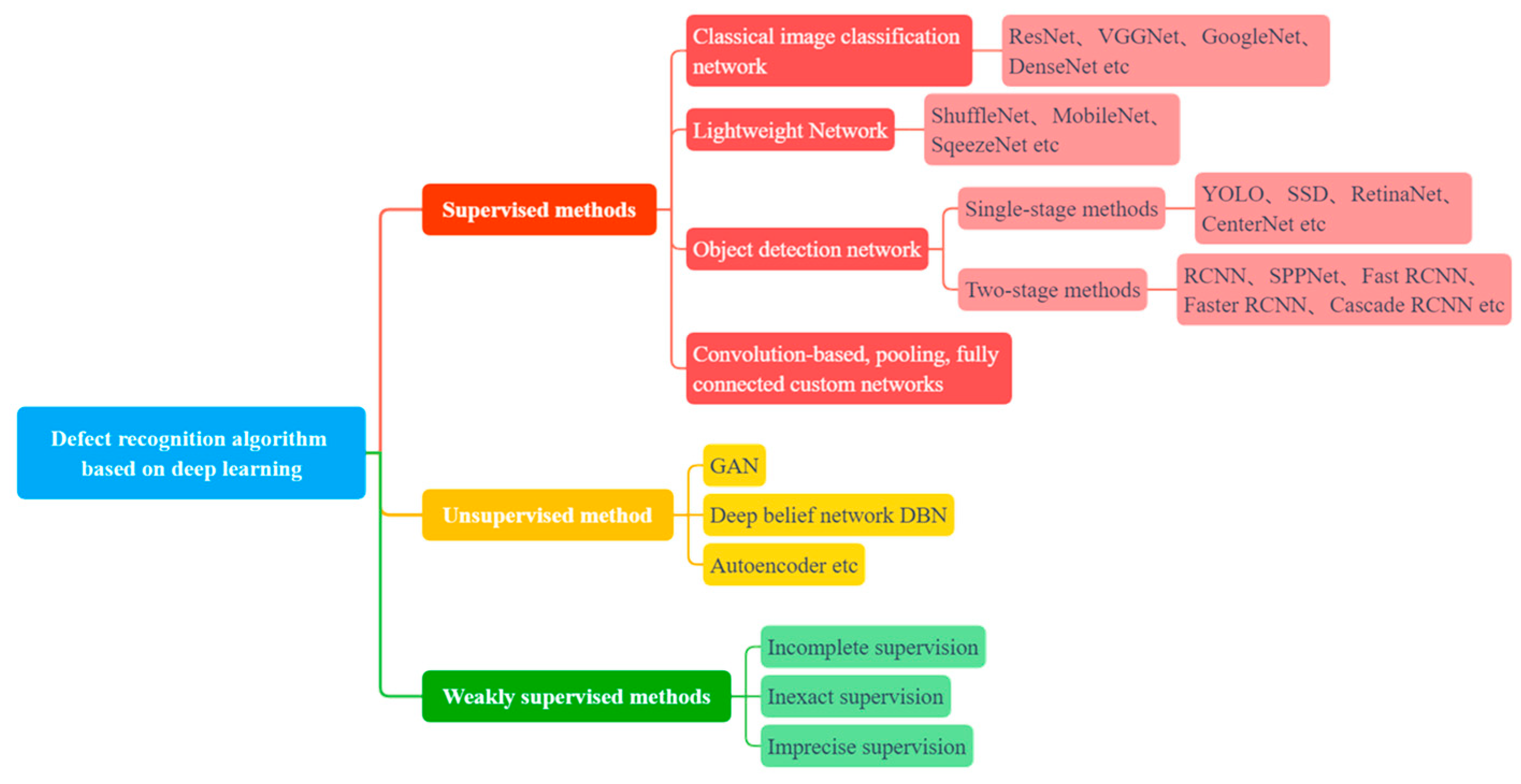
3.2. Defect Recognition Algorithm Based on Deep Learning

With the increase in computing power and the excellent performance of deep learning methods, many researchers have applied deep learning methods to various industrial inspection scenarios, and they have become the mainstream defect detection methods. Compared with traditional machine learning methods, deep learning methods can extract deeper and more abstract image features through operations such as convolution and pooling, and thus have more powerful characterization capabilities and do not require human-designed feature extraction rules, allowing for end-to-end model design. Convolutional neural networks use convolutional operations to extract features from input images, which can capture different levels of semantic information, thus effectively learning feature representations from a large number of samples and making the model have more powerful generalization capabilities. In addition, CNNs using pooling layers and sparse connections can reduce the model parameters while ensuring the efficiency of computational resources and network performance [78]. A detailed classification based on deep learning methods is shown in Figure 5.

3.2.1. Supervised Methods

Supervised methods of deep learning require well-labeled training sets and test sets to verify the performance of the methods, which are generally more stable and accurate than other types of methods. However, the quality of the training set directly affects the performance of the algorithm and in a real industrial defect detection scenario, it is very difficult to produce a well-labeled and large dataset. Fu et al. [79] proposed a fast and robust lightweight network model based on SqueezeNet, which emphasizes the learning of low-level features and adds an MRF module, thus achieving accurate recognition of defect types using a small number of defect samples, and it is worth mentioning that the recognition efficiency of this work exceeded 100 fps. The classification-first framework proposed by He et al. [80] in 2019 consists of two networks: the classification network MG-CNN and YOLO, where the MG-CNN is used to detect defect categories, and then the set of feature maps with defects present is fed to the YOLO network to determine the defect locations based on the results of the classification. In 2020, Ihor et al. [81] verified through experiments that the pre-trained model ResNet50 was the best choice as a classification network for detecting steel surface defects and used binary focus loss to alleviate the problem of data sample imbalance to realize the recognition of steel surface defects. Li et al. [82] designed a scheme combining domain adaptive and adaptive convolutional neural networks, DA-ACNN, for the identification of steel surface defects. In 2021, Feng et al. [83] adopted a scheme combining the RepVGG algorithm and spatial attention mechanism to realize the recognition of surface defects of a hot rolled strip. A new defect dataset X-SDD for a hot rolled strip was proposed. However, the recognition efficiency was not high because of the large number of parameters. In the same year, [4] trained Unet and Xception separately as classifiers to detect surface defects on rolled parts using synthetic datasets, and the normal dataset training was used as a reference to verify the feasibility and effectiveness of manually generated datasets. In 2021, Wang et al. [35] improved the VGG19 model, which is shown in Figure 6, and the scheme was divided into two parts: online detection and offline training. The online part extracts the ROI regions of the defect images using the improved grayscale projection algorithm, and then detects the strip surface defects using the improved VGG19 model; the offline part adds the extracted ROI regions to the defect dataset and performs ROI image augmentation, adds the results to the balanced mixed dataset, and then uses the mixed dataset training to improve the performance of VGG19, thus effectively solving the problem of few samples or an unbalanced dataset.
Pan, Y et al. [37] incorporated the dual-attention module into DeepLabv3+, and Xception was selected as the network to achieve accurate to pixel-level defect localization segmentation. The edge-aware multilevel interaction network proposed by Zhou et al. in 2021 [84] used the ResNet network as the base backbone and adopted a U-shaped architecture composed of encoder decoders to recognize strip surface defects. In 2022, Liu et al. [85] designed the lightweight network CASI-Net, whose structure is shown in Figure 7. The network uses a lightweight feature extractor to extract image features, and then uses a collaborative attention mechanism and self-interaction module based on a biological vision to modify the features. Finally, multilayer perceptron (MLP) was used to classify the surface defects of the steel strip.

3.2.2. Unsupervised Methods

Unsupervised methods, as opposed to supervised methods, do not require their training sets to be labeled, or are even just trained with enough defect-free samples, making up for the disadvantage that supervised methods have difficulty in producing datasets. However, in contrast, the detection accuracy of unsupervised methods is generally lower than that of supervised methods, and there is instability in the training results. The commonly used unsupervised methods include autoencoder, GAN, deep belief network [86,87], and self-organizing graph [88], etc. In 2017, Liu et al. [89] used an anisotropic diffusion model to eliminate the interference of pseudo-defects, then proposed a new HWV unsupervised model to characterize the texture distribution of each local block in the image, and finally invoked the adaptive thresholding technique to achieve the segmentation of the defects and background. Mei et al. (2018) [90] also used only defect-free samples to train the model, and the method was constructed based on the convolutional denoising autoencoder (CDAE) architecture of Gaussian pyramids to distinguish between defective and defect-free parts. In 2019, [91] proposed a single classification method based on GAN for steel strip surface defect detection, which could only detect the presence or absence of defects and cannot distinguish the categories. In the same year, [92] used convolutional autoencoder convolutional autoencoder (CAE) and sharpening processing to extract the defect features of the missing input image, and finally used Gaussian blurring and thresholding as post-processing to clarify the defects to achieve the segmentation of defects. In 2020, Niu et al. [93] proposed a global low-rank non-negative reconstruction algorithm with background constraints to fuse the detection results of 2D significant maps and 3D contour information to achieve the detection of rail surface defects.

3.2.3. Weakly Supervised Methods

Weakly supervised methods between supervised and unsupervised methods, which have three categories, namely, incomplete supervision, inexact supervision, and imprecise supervision [94]. The first two of these methods have both been well validated in the field of surface defect detection. Among them, inexact supervision refers to the use of a small amount of labeled data mixed with a large amount of unlabeled data for training, so that a more desirable accuracy can be obtained while avoiding the difficulty of producing a large number of labeled datasets. Uncertain supervision is the use of a small amount of fully labeled data (pixel-level labeling) mixed with a large amount of weakly labeled data (image-level or box-level), which showed a performance almost as good as that of fully supervised methods and reduced the trouble of producing fully labeled datasets. Finally, inaccurate supervision means that the given data samples may contain partially incorrect labeling information. The scheme proposed by He et al. [95] in 2019 combined a convolutional autoencoder with a semi-supervised GAN and introduced a passthrough layer in the CAE to extract fine-grained features, resulting in excellent recognition accuracy. In 2019, the Google Institute [96] designed a new algorithm MixMatch by unifying the current mainstream semi-supervised algorithms, and conducted extensive detection experiments using this algorithm, which will have a significant performance improvement compared with other weakly supervised methods. He et al. [97] proposed a multiple learning algorithm based on the GAN and ResNet18 networks, which could generate data samples by itself and provide labels for the samples, enabling the expansion of the dataset, thus further enhancing the recognition of defects with few samples. Jong et al., 2020 [98] proposed a new convolutional variational autoencoder, convolutional variational autoencoder (CVAE), which was used to generate defect images and then used these images to train the proposed CNN classifier to achieve high accuracy defect detection. The model designed by Jakob et al. (2021) [99] had two sub-network architectures [100,101], a segmentation sub-network that learns from pixel-level labels, and a classification sub-network that learns from weak image-level labels and combines these two networks to achieve hybrid supervision, and experimentally demonstrated that hybrid supervised training with only a few fully annotated samples added to weakly labeled image samples could yield comparable performance to the fully supervised model. Zhang et al. [102] proposed a weakly supervised learning method named CADN, which was implemented by extracting the category perception spatial information from the classification pipeline, only used weak image labels for training, and could simultaneously realize image classification and defect localization.
To facilitate the understanding of the characteristics of the three deep learning methods, a pipeline diagram of the deep learning methods is summarized in Figure 8 and the characteristics of the deep learning methods are shown in Table 4.

3.3. Object Detection Methods

The counterpart of the image classification network is the object detection network, which mainly contains single-stage methods and two-stage methods, each of which has its own advantages and disadvantages. The main difference between the single-stage and two-stage methods is whether there is a clear candidate box generation stage within the algorithm. The single-stage object detection algorithm directly calculates the image to generate the detection result, which is fast, but the detection accuracy is relatively low; the two-stage object detection algorithm first extracts the candidate box from the image, and then conducts the secondary correction based on the candidate region to obtain the detection point result, which has a higher detection accuracy, but slower detection speed. Therefore, what needs to be done in the field of object detection is to continuously optimize the mainstream object detection algorithms to achieve the best balance of detection accuracy and speed.

3.3.1. Single-Stage Methods

The most popular single-stage algorithms include SSD [24], YOLO [27], RetinaNet [28], CenterNet [33], etc. Li et al. [103] used a fully convolutional YOLO network to achieve the classification and localization of surface defects in steel strip with high recognition accuracy and speed. Yang et al. [104] proposed a deep learning algorithm for the defect detection of tiny parts based on a single short detector network SSD and speed model with a maximum detection accuracy of 99%. In 2021, Cheng et al. [105] proposed a steel surface defect recognition scheme based on RetinaNet with differential channel attention and adaptive spatial feature fusion (ASFF). Kou et al. [106] proposed an end-to-end defect detection model based on YOLO-V3 and combined it with anchor free feature selection to reduce the computational complexity of the model. However, this work could only detect defects in the normal size range, and very small defects in high-resolution images could not be detected. In 2022, Chen et al. [107] proposed a real-time surface defect detection method based on YOLO-V3 with a lightweight network MobileNeV2 selected for its backbone network, an extended feature pyramid network (EFPN) was proposed to detect multi-size objects, a feature fusion module was also designed to capture more regional details, and the scheme achieved high detection speed and accuracy. Tian et al. [108] proposed a steel surface defect detection algorithm called DCC-CenterNet, which not only focused on the center of the defect, but also extracted the overall information without drawing false attention.

3.3.2. Two-Stage Methods

In the field of industrial defect detection, common two-stage classical methods include RCNN [21], SPPNet [20], Fast RCNN [23], Faster RCNN [26], and Cascade RCNN [29], etc. The method proposed by Rubo et al. in 2020 [109] was based on Faster R-CNN and proposed three important improvements of weighted ROI pooling, FPN-based multi-scale feature extraction network, and strict-NMS to achieve more accurate defect recognition. Wang et al. in 2021 [36] proposed a combination of ResNet50 and an improved Faster R-CNN algorithm to detect steel surface defects and proposed three important improvements to the Faster R-CNN with spatial pyramid pooling (SPP), enhanced feature pyramid network (FPN), and matrix NMS algorithm to achieve higher detection accuracy. Zhao et al. [110] proposed an improved Faster R-CNN based network model, whose model structure is shown in Figure 9, where ResNet50 is used as the feature extraction network. First, the ResNet-50 network is reconstructed using deformable convolution. Second, the feature pyramid network is used to fuse multi-scale features and replace the fixed region of interest pooling layer with a variable pooling layer. Finally, the soft non-maximum value suppression algorithm (SNMS) is used to suppress detection frames that have significant overlap with the highest score detection frames, thereby enhancing the network’s ability to identify defects. The method proposed by Li et al. [8] in 2022 is based on the improved YOLOV5 and Optimized-Inception-ResNetV2 models, where the first stage is to locate defects with the improved YOLOV5, and the second stage is to extract defect features and classify them with Optimized-Inception-ResNetV2. A summary of deep learning-based methods for identifying steel surface defects is shown in Table 5.

4. Datasets and Performance Evaluation Metrics

4.1. Datasets

Datasets are the basis of research work on steel surface defect recognition. A good dataset is more conducive to problem identification, thus facilitating problem solving. With the improvements at the industrial manufacturing level, the number of defective products is becoming smaller and smaller, so it is very challenging to create a high-quality dataset for the training of aa defect recognition algorithm. In addition, the labeling of data samples is also more labor-intensive. A high-quality dataset is very important for the defect recognition algorithm, which will directly affect the final performance of the algorithm. Therefore, the commonly used publicly available datasets have been summarized in the field of steel surface defect recognition. Most of the selected datasets were steel surface defect datasets, but they also contain some texture datasets of various materials for future researchers. A summary of the datasets in the field of industrial product defect detection is shown in Table 6.

4.2. Defect Recognition Algorithm Performance Evaluation Metrics

The performance evaluation metrics of defect recognition algorithms were used to measure the performance of the designed algorithms, and the selection of the algorithm performance evaluation metrics should be comprehensive because the selection of different evaluation metrics may present different results. This paper summarizes some of the algorithm performance evaluation metrics commonly used in the field of steel defect detection, which can be broadly divided into two categories: the precision class metrics and the efficiency class metrics.

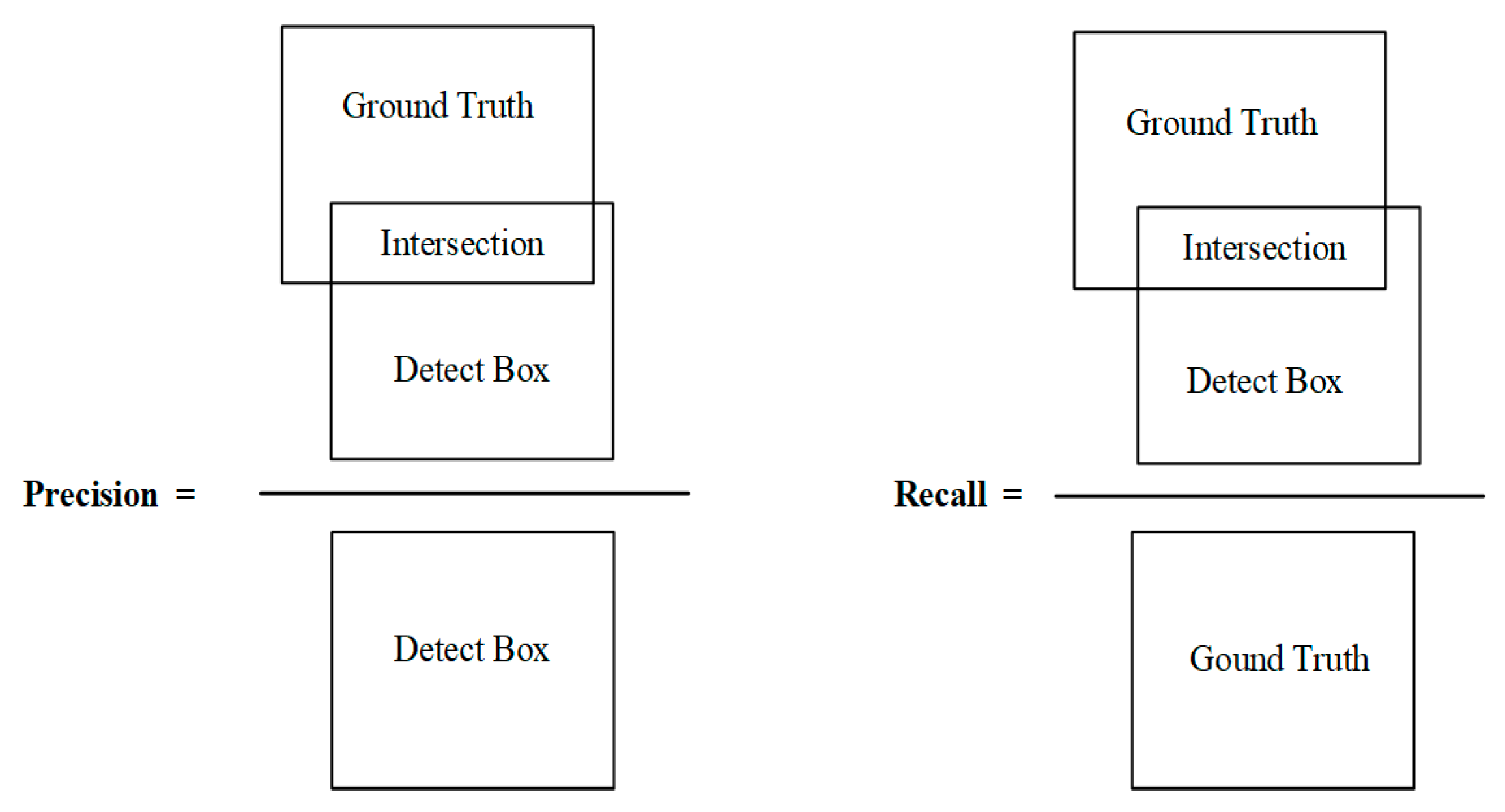
4.2.1. The Precision Class Metrics

The precision class evaluation metrics were used to evaluate the precision of the relevant algorithms for the classification of defect categories and the precision of the defect localization segmentation.
The first and most basic evaluation metrics are TP, TN, FP, and FN, where TP indicates the true positive, the number of correctly classified positive samples; TN indicates the true negative, the number of correctly classified negative samples; FP indicates the false positive, the number of negative samples classified as positive; and FN indicates the false negative, the number of positive samples classified as negative. Based on the above four basic evaluation metrics, evaluation metrics such as PRE, RECALL, ACC, false escape rate, and false alarm rate evolved. Among them, PRE represents the ratio of the number of correctly predicted positive samples to the number of predicted positive samples, the classification precision of the algorithm, with the following equation:
P R E = T P T P + F P ,
A higher PRE means a smaller random error, a smaller variance, describing the perturbation of the prediction results. RECALL indicates the ratio of the number of correctly predicted positive samples to the number of actual positive samples, which is given by the following formula:
R E C A L L = T P T P + F N ,
A higher value of RECALL means that the algorithm is more capable of detecting the object algorithm. ACC indicates the proportion of the total number of correctly predicted samples to the total number of samples, which is given by the following formula:
A C C = T P + T N T P + T N + F P + F N ,
A higher value of ACC represents a smaller systematic error, a smaller deviation, and describes the degree of deviation of the predicted result from the actual value. For the error escape rate, EE is defined as the number of negative samples judged to be positive as a proportion of the total number of negative samples in the sample, calculated as follows:
E E = F P T N + F P ,
For the false alarm rate, FA is defined as the ratio of the number of positive samples incorrectly determined as negative to the number of all positive samples, calculated as follows:
F A = F N T P + F N ,
It should be noted that the above metrics, if the values of the evaluation metrics of a single category are calculated in the multi-classification algorithm, it is necessary to take any of the classes in the multi-classification as a positive sample and combine the other classes into one class as a negative sample, so that the TP, TN, FP, and FN of each class can be calculated separately, and thus the other evaluation metrics of each class can be calculated. The formula of PRE and RECALL shows that the higher the PRE indicator, the higher the accuracy of predicting positives, but this indicator does not take into account the wrong prediction of negative samples, while the RECALL indicator is exactly the opposite situation, that is, it does not take into account the wrong prediction of positive samples, so it is possible that there is an algorithm with very high and very low PRE and RECALL metrics. A good algorithm also needs to have both a high PRE and RECALL. Therefore, a metric that integrates PRE and RECALL is needed, and the F-measure can meet this requirement with the following formula:
F m e a s u r e = ( 1 + β 2 ) P R E R E C A L L β 2 P R E + R E C A L L ,
When β = 1, the F-measure is the F1-score. The evaluation metric WF is the weighted F-measure, which is calculated as follows:
W F = ( 1 + β 2 ) P R E w × R E C A L L w β 2 P R E w + R E C A L L w ,
For the AP and mAP metrics, they are also calculated based on PRE and RECALL, where the AP average precision is defined by calculating the area under the P–R curve, and by changing different confidence thresholds, multiple pairs of PRE and RECALL, values can be obtained where the P–R curve is defined by putting the RECALL value on the X-axis and the PRE value on the Y-axis, resulting in a PRE–RECALL curve, referred to as the P–R curve. For the AP calculation method, the average accuracy calculation method is generally calculated by 11-point interpolation, and the calculation formula is as follows:
A P = 1 11 × i { 0 , 0.1 , , 1 } A P r ( i ) ,
Once the AP for all categories have been calculated, the value of the average precision mAP for all categories can be calculated with the following formula:
m A P = i = 1 K A P i K ,
where K refers to the number of categories. Similar to the AP calculation is the AUC, which means the area under the ROC curve, and a higher value of AUC means a better effect of the corresponding classifier. The ROC curve is also called the perceptivity curve, and the horizontal coordinate of the curve is the FPR, which is the false positive rate, and the vertical coordinate is the TPR, which is the true positive rate. The AUC calculation formula is as follows:
A U C = i p o s i t i v e c l a s s r a n k i M × ( M + 1 ) 2 M × N ,
where i p o s i t i v e c l a s s r a n k i refers to the summation of each positive sample serial number located in the position after the subtraction operation (according to the probability of the score from the small to reach the ranking, ranked in the rank position); M   and N are the number of positive and negative samples, respectively. MAE and MSE represent the average absolute error and mean square error, respectively, and when both two-evaluation metrics are smaller, it represents the better performance of the algorithm, where the MAE is calculated as follows:
M A E = 1 n i = 1 n | y ^ i y i | ,
The MSE calculation formula is as follows:
M S E = 1 n i = 1 n ( y ^ i y i ) 2 ,
where y ^ i indicates actual value and y i indicates the predicted value.
For the object detection algorithm, PRE and RECALL are defined in a different way to that in the above statement. The PRE in the object detection algorithm is the percentage of the ratio of the overlapping area size of Ground Truth and the actual localization result to the area size of the actual localization result. RECALL is the percentage of the ratio of the overlapping area size of Ground Truth and the actual localization result to the area size of Ground Truth. The calculation process is shown in Figure 10.
In addition, the calculation of MAE and MSE is slightly different from the above description, but the meaning is the same, so the MAE and MSE calculation formulae are as follows:
M A E = 1 W × H i = 1 W × H | S ( i ) G T s ( i ) | ,
M S E = 1 W × H i = 1 W × H ( S ( i ) G T s ( i ) ) 2
where W and H denote the height and width of the localized segmentation area, respectively; S denotes the area of the localized segmentation area; and G T S denotes the actual defect area. The Dice coefficient, IoU, is also used as an evaluation metric in the object detection algorithm. The Dice coefficient is used to compare the pixel consistency between the predicted segmentation results and their corresponding G T S , and is calculated as follows:
D i c e ( X , Y ) = 2 × | X Y | | X | + | Y | ,
IoU, which reflects the detection effect of the predicted detection frame and the real detection frame, has a very good characteristic of scale invariance, that is, it is scale insensitive, and the calculation formula is as follows:
I o U = | X Y | | X Y | ,
where X denotes the segmentation result and Y denotes G T S . SM [126] can evaluate the structural similarity between the saliency map S and GTs by considering both the values of region perception Sr and object perception So, which can be defined as:
S M = α × S o + ( 1 α ) × S r ,
where α denotes the balance parameters, which are typically set to 0.5. Finally, PFOM [127] visualizes the boundary quality of the segmentation result, which is commonly used in the edge detection region and can be defined as:
P F O M = 1 max ( N G , N S ) k = 1 N S 1 1 + α d k 2 ,
where N G denotes the number of ideal edge points extracted from the GTS and N S denotes the actual number of edge points of the segmentation result. α denotes the scaling constants that are typically set to 0.1 or 1/9; d k denotes the Euclidean distance between the kth true edge point and the detected edge point.

4.2.2. The Efficiency Class Metrics

The efficiency metric is used to evaluate the speed of the relevant algorithm to recognize defects, which can directly reflect whether the algorithm can achieve the ability to identify the product surface defects in real-time on the production line as well as the complexity of the algorithm design.
Commonly used efficiency class metrics include training duration, testing duration, parameters Params, Inference Time, FPS, FLOPs, etc. Among them, training duration and testing duration are the most easily to obtain and intuitive data in the process of algorithm experiments. However, due to the different hardware environment of each work, even if the same method is used, the length of time measured is also different when training and testing on different hardware conditions, which needs to be considered by other efficiency evaluation metrics. Params refers to the number of parameters involved in the calculation of the designed method. This index reflects the amount of memory occupied by the designed method, and its unit is generally represented by M. The Inference Time and FPS are the corresponding evaluation metrics. The former refers to the time spent to detect an image, the unit of which is generally MS; the latter is the number of images that can be detected within one second, also known as the number of frames. FLOPs represents the computing complexity, which describes the complexity of the algorithm and reflects the hardware requirement of the designed algorithm. The unit of FLOPs is usually denoted by B.

5. Challenges and Solutions

This section presents four challenges in the field of steel surface defect detection: the problem of insufficient data samples, the problem of unbalanced data samples, the problem of real-time detection, and the problem of small object detection, and gives appropriate recommendations for solving them.

5.1. The Problem of Insufficient Data Samples

In terms of deep learning algorithms, generally the deeper the level, the better the performance of deep neural networks, but they require a large amount of data for training, otherwise they are prone to overfitting due to the high number of parameters in very deep networks. However, the quality of datasets in the real environment is generally not high and the number of types is not complete, resulting in deep neural networks not being able to give full play to their performance when performing defect detection. To address this problem, there are four effective solutions that can be used in combination with the following. The first is the use of transfer learning methods, which use transfer learning techniques to migrate pre-trained models (e.g., ResNet, VGG, etc.) that have been trained in large datasets to the object detection problem (which usually has a smaller training dataset). Transfer learning relaxes the assumption that the training data must be independent and identically distributed with the test data [128], but it may affect the final algorithm performance because the initial training dataset of the pre-trained model has a large gap with the images for defect detection. Next, unsupervised or weakly supervised methods can be chosen as a way to alleviate the problem of an insufficient and incomplete number of defect samples in the dataset. Detailed descriptions of unsupervised and weakly supervised methods can be found in Section 3.2.2 and Section 3.2.3 in this paper. Data augmentation techniques can also be used to expand the dataset to alleviate the problem of insufficient dataset. Data augmentation techniques are very flexible and can be used in the preparation phase of the dataset prior to training or can be performed automatically during training [129]. Common methods of data augmentation include performing image transformation operations such as random cropping, scaling, color shifting, flipping, mirroring, and scaling to pre-process the original image for the purpose of extending the original dataset. Finally, the problem of insufficient data samples is solved by optimizing the network structure such as the proposed GAN network model, which generates the image closest to the test image by continuously optimizing the parameters of the iterative generator G. Then, the defect recognition algorithm is trained based on this, so in the field of surface defect recognition, there are many methods based on GAN networks for image defect recognition methods such as in [130,131].

5.2. The Problem of Unbalanced Data Samples

In deep learning-based defect detection algorithms, when performing model training, the required dataset usually requires the number of sample sets of each category in the dataset to be almost the same. However, the actual situation is that the number of defect-free samples in the dataset is the largest, and the defective samples only account for a small portion, or the number of samples in the defective samples is very unevenly distributed among the various defective categories, and the number of easily collected defective samples accounts for the majority, a situation known as data sample imbalance. This imbalance exists in supervised learning methods, which will directly lead the algorithm to put more attention on the categories with more sufficient samples in the dataset and less recognition ability for the categories with smaller data volume, thus affecting the recognition ability of the algorithm for each type of defect. To address the problem of data sample imbalance, the following methods can be used to solve it. First, at the dataset level, data augmentation, data resampling [132], and GAN networks can be used to change the sample distribution of the training set to a balanced state. Second, at the model level, the attention to small samples can be adjusted by assigning appropriate weights to each sample in the training set, assigning higher weights to a smaller number of sample categories, and lower weights to a larger number of sample categories, and then the objective function can be optimized by increasing the loss term for small classes of misclassified samples in the objective function. In addition, the anomaly detection algorithm can be referred to build a single classifier for anomalies (categories with small sample size) to detect them, thus solving the data sample imbalance problem.

5.3. Real-Time Detection of Problems

In many real industrial scenarios of defect detection tasks, real-time detection is required such as online analysis and online monitoring, which requires a millisecond response speed. Therefore, the ability to perform real-time detection is a very important consideration for the practicality of the algorithm, but the defect recognition algorithm still faces the contradiction of accuracy and speed. For the time being, increasing the detection efficiency of the model can be considered from two aspects: the algorithm and hardware. In terms of algorithms, there is an option to use and develop some lightweight detection algorithms such as SqueezeNet [25], MobileNet [31], and ShuffleNet [32], etc. by trying to improve the recognition speed of the two-stage algorithm or the recognition accuracy of the single-stage algorithm, aiming to achieve the lowest balance between the lowest computational cost and the highest accuracy. In addition, model acceleration can be performed by using optimized convolutional operations or by using distillation, pruning and dropout techniques. On the hardware side, GPUs, FPGAs, DSPs, and Google’s TPUs can be used to speed up the model computation.

5.4. The Problem of Small Object Detection

For small object detection, there are two definitions: first, the absolute size is small, and it is generally considered that the object size to be detected is smaller than 32 × 32 pixels will be recognized as small; the other is the relative size is small, that is, the ratio of the object size to the original image size to be detected is less than 0.1, and it will be recognized as small. The problem of small object detection can be optimized from the following aspects: first, feature fusion technology can be used to fuse deep semantic information into shallow feature maps, while using the rich semantic information of deep features and shallow features to achieve the detection of small objects. Second, one can choose to set the input size of the image by scaling the input image to an appropriate scale and then inputting it into the network for detection. Context information can also be used to establish a connection between the object and its context. Finally, one can also choose to reduce the downsampling rate of the network to reduce the loss of detection objects on the feature map; this reduction in the loss of information is beneficial to the detection of small objects, and common methods are to reduce the pooling layer and use the null convolution.

6. Summary and Future Work

Steel is the core material of the world’s industrial production, and the development of steel surface defect recognition technology promotes the high-quality production of steel. Therefore, the research on steel surface defect recognition technology is of great importance worldwide. The various types of defect recognition methods summarized in Section 3 of this paper have been published in the last 10 years, and most of them have been published in the last 5 years and represent the best performance methods in this field. First, this paper summarized the difficulties of steel surface defect recognition, and then counted the surface types of steel and the corresponding surface defect categories. Second, we presented a detailed comparison of the key hardware of the surface defect detection system. This paper presented a systematic classification of steel surface defect recognition algorithms, a literature review for each category, and a summary of the characteristics of each technique. Since there is a lack of large and uniform datasets in the field of steel surface defect recognition, and many methods have different performance evaluation metrics, several commonly used public datasets were summarized and more than 20 performance evaluation metrics were aggregated. Finally, the challenges faced by the current steel surface defect recognition technology are summarized and corresponding solutions are proposed. The goal of this paper was to facilitate the future research efforts of those studying steel surface defect recognition techniques.
In future work, we aim to create a public algorithm performance evaluation platform for steel surface defect recognition, where researchers can make a fair and comprehensive comparison of various steel surface defect recognition algorithms, which will greatly contribute to the development of steel surface defect recognition technology. The platform will provide a complete steel surface defect dataset, a code based on current mainstream public algorithms, a comprehensive set of algorithm performance evaluation metrics, and a software toolkit and interface for researchers to upload new algorithm codes for testing on their own. In addition to building an algorithm evaluation platform, we will design a weakly supervised learning algorithm. We believe that the weakly supervised learning algorithm will become the mainstream algorithm for steel defect recognition in the future because it maintains a similar accuracy and stability of training results to the supervised learning algorithm while significantly reducing the demanding dataset requirements. We will focus our research on weakly supervised learning algorithms in two directions: reducing the algorithm complexity and improving the defect detection efficiency.

Author Contributions

Conceptualization, X.W.; Methodology, J.S.; Validation, J.S. and X.W.; Formal analysis, Y.H.; Investigation, J.S. and X.W.; Resources, K.S.; Data curation, K.S.; Writing—original draft preparation, X.W., J.S., Y.H. and K.S.; Writing—review and editing, X.W., J.S., Y.H. and K.S.; Visualization, J.S. and Y.H.; Supervision, K.S.; Project administration, X.W.; Funding acquisition, X.W. All authors have read and agreed to the published version of the manuscript.

Funding

This research was funded by Liaoning Provincial Department of Education Scientific Research Project, grant number LQGD2020023.

Institutional Review Board Statement

Not applicable.

Informed Consent Statement

Not applicable.

Data Availability Statement

Not applicable.

Conflicts of Interest

The authors declare no conflict of interest.

References

  1. Basson, E. World Steel in Figures 2022. Available online: https://worldsteel.org/steel-topics/statistics/world-steel-in-figures-2022/ (accessed on 30 April 2022).
  2. Jain, S.; Seth, G.; Paruthi, A.; Soni, U.; Kumar, G. Synthetic data augmentation for surface defect detection and classification using deep learning. J. Intell. Manuf. 2020, 33, 1007–1020. [Google Scholar] [CrossRef]
  3. He, Y.; Song, K.; Meng, Q.; Yan, Y. An end-to-end steel surface defect detection approach via fusing multiple hierarchical features. IEEE Trans. Instrum. Meas. 2019, 69, 1493–1504. [Google Scholar] [CrossRef]
  4. Luo, Q.; Fang, X.; Su, J.; Zhou, J.; Zhou, B.; Yang, C.; Liu, L.; Gui, W.; Lu, T. Automated Visual Defect Classification for Flat Steel Surface: A Survey. IEEE Trans. Instrum. Meas. 2020, 69, 9329–9349. [Google Scholar] [CrossRef]
  5. He, Y.; Wen, X.; Xu, J. A Semi-Supervised Inspection Approach of Textured Surface Defects under Limited Labeled Samples. Coatings 2022, 12, 1707. [Google Scholar] [CrossRef]
  6. Ma, S.; Song, K.; Niu, M.; Tian, H.; Yan, Y. Cross-scale Fusion and Domain Adversarial Network for Generalizable Rail Surface Defect Segmentation on Unseen Datasets. J. Intell. Manuf. 2022, 1–20. [Google Scholar] [CrossRef]
  7. Wan, C.; Ma, S.; Song, K. TSSTNet: A Two-Stream Swin Transformer Network for Salient Object Detection of No-Service Rail Surface Defects. Coatings 2022, 12, 1730. [Google Scholar] [CrossRef]
  8. Li, Z.; Tian, X.; Liu, X.; Liu, Y.; Shi, X. A Two-Stage Industrial Defect Detection Framework Based on Improved-YOLOv5 and Optimized-Inception-ResnetV2 Models. Appl. Sci. 2022, 12, 834. [Google Scholar] [CrossRef]
  9. Song, K.; Wang, J.; Bao, Y.; Huang, L.; Yan, Y. A Novel Visible-Depth-Thermal Image Dataset of Salient Object Detection for Robotic Visual Perception. IEEE/ASME Trans. Mechatron. 2022. [Google Scholar] [CrossRef]
  10. Sun, G.; Huang, D.; Cheng, L.; Jia, J.; Xiong, C.; Zhang, Y. Efficient and Lightweight Framework for Real-Time Ore Image Segmentation Based on Deep Learning. Minerals 2022, 12, 526. [Google Scholar] [CrossRef]
  11. Neogi, N.; Mohanta, D.K.; Dutta, P.K. Review of vision-based steel surface inspection systems. EURASIP J. Image Video Process. 2014, 2014, 50. [Google Scholar] [CrossRef]
  12. Verlag Stahleisen GmbH, Germany. Available online: www.stahleisen.de (accessed on 13 June 2022).
  13. Viola, P.; Jones, M.J. Robust real-time face detection. Int. J. Comput. Vis. 2004, 57, 137–154. [Google Scholar] [CrossRef]
  14. Dalal, N.; Triggs, B. Histograms of oriented gradients for human detection. In Proceedings of the 2005 IEEE Computer Society Conference on Computer Vision and Pattern Recognition (CVPR’05), San Diego, CA, USA, 20–25 June 2005; IEEE: Piscatevi, NJ, USA, 2005; 1, pp. 886–893. [Google Scholar]
  15. Felzenszwalb, P.F.; Girshick, R.B.; McAllester, D.; Ramanan, D. Object detection with discriminatively trained part-based models. IEEE Trans. Pattern Anal. Mach. Intell. 2010, 32, 1627–1645. [Google Scholar] [CrossRef] [PubMed] [Green Version]
  16. Krizhevsky, A.; Sutskever, I.; Hinton, G.E. Imagenet classification with deep convolutional neural networks. Commun. ACM 2017, 60, 84–90. [Google Scholar] [CrossRef] [Green Version]
  17. Goodfellow, I.; Pouget-Abadie, J.; Mirza, M.; Xu, B.; Warde-Farley, D.; Ozair, S.; Courville, A.; Bengio, Y. Generative adversarial networks. Commun. ACM 2020, 63, 139–144. [Google Scholar] [CrossRef]
  18. Simonyan, K.; Zisserman, A. Very deep convolutional networks for large-scale image recognition. arXiv 2014, arXiv:preprint,1409,1556. [Google Scholar]
  19. Szegedy, C.; Liu, W.; Jia, Y.; Sermanet, P.; Reed, S.; Anguelov, D.; Rabinovich, A. Going deeper with convolutions. In Proceedings of the IEEE Conference on Computer Vision and Pattern Recognition, Boston, MA, USA, 7–12 June 2015; pp. 1–9. [Google Scholar]
  20. He, K.; Zhang, X.; Ren, S.; Sun, J. Spatial pyramid pooling in deep convolutional networks for visual recognition. IEEE Trans. Pattern Anal. Mach. Intell. 2015, 37, 1904–1916. [Google Scholar] [CrossRef] [Green Version]
  21. Girshick, R.; Donahue, J.; Darrell, T.; Malik, J. Rich feature hierarchies for accurate object detection and semantic segmentation. In Proceedings of the IEEE Conference on Computer Vision and Pattern Recognition, Columbus, OH, USA, 23–28 June 2014; pp. 580–587. [Google Scholar]
  22. He, K.; Zhang, X.; Ren, S.; Sun, J. Deep residual learning for image recognition. In Proceedings of the IEEE Conference on Computer Vision and Pattern Recognition, Las Vegas, NV, USA, 27–30 June 2016; pp. 770–778. [Google Scholar]
  23. Girshick, R. Fast r-cnn. In Proceedings of the IEEE International Conference on Computer Vision, Santiago, Chile, 7–13 December 2015; pp. 1440–1448. [Google Scholar]
  24. Liu, W.; Anguelov, D.; Erhan, D.; Szegedy, C.; Reed, S.; Fu, C.Y.; Berg, A.C. Ssd: Single shot multibox detector. In European Conference on Computer Vision; Springer: Cham, Switzerland, 2016; pp. 21–37. [Google Scholar]
  25. Iandola, F.N.; Han, S.; Moskewicz, M.W.; Ashraf, K.; Dally, W.J.; Keutzer, K. SqueezeNet: AlexNet-level accuracy with 50x fewer parameters and<0.5 MB model size. arXiv 2016, arXiv:preprint. 1602.07360. [Google Scholar]
  26. Ren, S.; He, K.; Girshick, R.; Sun, J. Faster r-cnn: Towards real-time object detection with region proposal networks. Adv. Neural Inf. Process. Syst. 2015, 28. [Google Scholar] [CrossRef] [Green Version]
  27. Redmon, J.; Divvala, S.; Girshick, R.; Farhadi, A. You only look once: Unified, real-time object detection. In Proceedings of the IEEE Conference on Computer Vision and Pattern Recognition, Las Vegas, NV, USA, 27–30 June 2016; pp. 779–788. [Google Scholar]
  28. Lin, T.Y.; Goyal, P.; Girshick, R.; He, K.; Dollár, P. Focal loss for dense object detection. In Proceedings of the IEEE International Conference on Computer Vision, Venice, Italy, 22–29 October 2017; pp. 2980–2988. [Google Scholar]
  29. Cai, Z.; Vasconcelos, N. Cascade r-cnn: Delving into high quality object detection. In Proceedings of the IEEE Conference on Computer Vision and Pattern Recognition, Los Alamitos, CA, USA, 18–22 June 2018; pp. 6154–6162. [Google Scholar]
  30. Huang, G.; Liu, Z.; Van Der Maaten, L.; Weinberger, K.Q. Densely connected convolutional networks. In Proceedings of the IEEE Conference on Computer Vision and Pattern Recognition, Honolulu, HI, USA, 21–26 July 2017; pp. 4700–4708. [Google Scholar]
  31. Howard, A.G.; Zhu, M.; Chen, B.; Kalenichenko, D.; Wang, W.; Weyand, T.; Adam, H. Mobilenets: Efficient convolutional neural networks for mobile vision applications. arXiv 2017, arXiv:preprint 1704.04861. [Google Scholar]
  32. Zhang, X.; Zhou, X.; Lin, M.; Sun, J. Shufflenet: An extremely efficient convolutional neural network for mobile devices. In Proceedings of the IEEE Conference on Computer Vision and Pattern Recognition, Los Alamitos, CA, USA, 18–22 June 2018; pp. 6848–6856. [Google Scholar]
  33. Duan, K.; Bai, S.; Xie, L.; Qi, H.; Huang, Q.; Tian, Q. Centernet: Keypoint triplets for object detection. In Proceedings of the IEEE/CVF International Conference on Computer Vision, Long Beach, CA, USA, 16–20 June 2019; pp. 6569–6578. [Google Scholar]
  34. Zheng, X.; Zheng, S.; Kong, Y.; Chen, J. Recent advances in surface defect inspection of industrial products using deep learning techniques. Int. J. Adv. Manuf. Technol. 2021, 113, 35–58. [Google Scholar] [CrossRef]
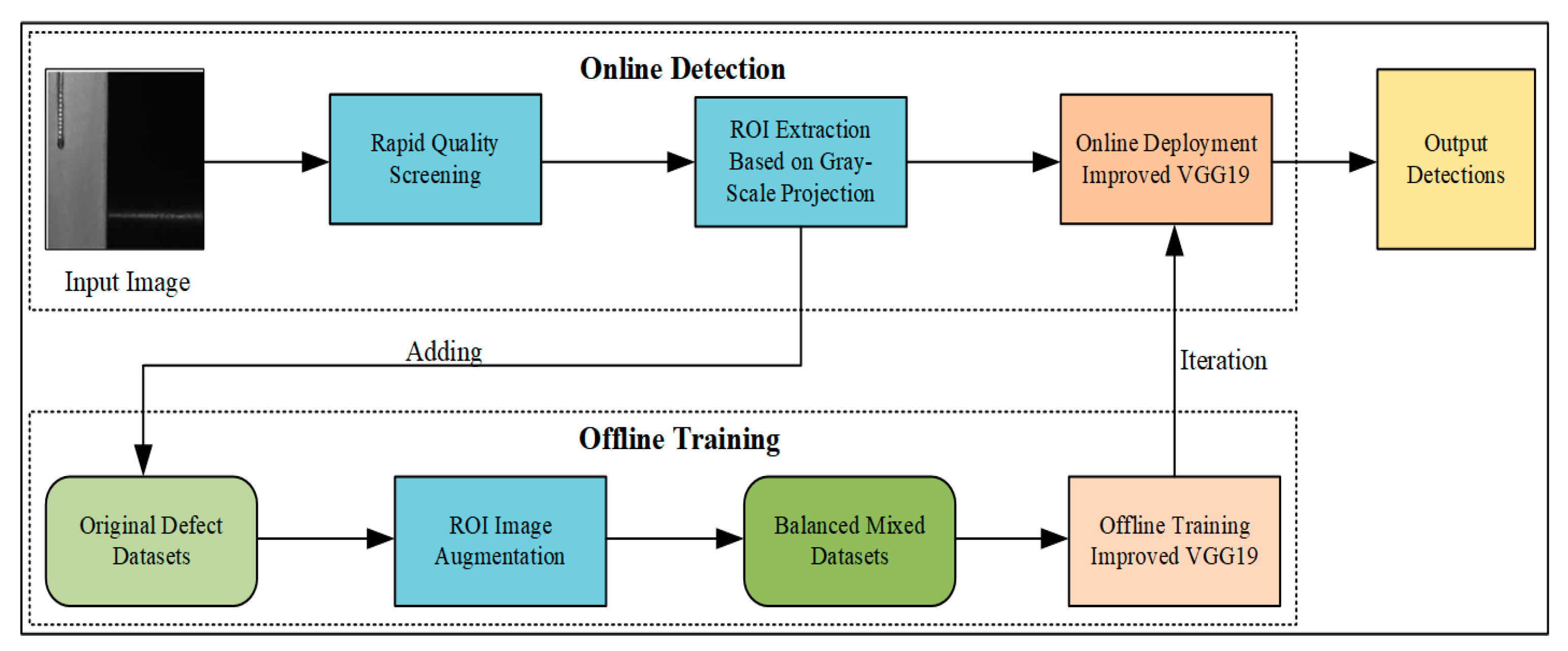
  35. Wan, X.; Zhang, X.; Liu, L. An Improved VGG19 Transfer Learning Strip Steel Surface Defect Recognition Deep Neural Network Based on Few Samples and Imbalanced Datasets. Appl. Sci. 2021, 11, 2606. [Google Scholar] [CrossRef]
  36. Wang, S.; Xia, X.; Ye, L.; Yang, B. Automatic detection and classification of steel surface defect using deep convolutional neural networks. Metals 2021, 11, 388. [Google Scholar] [CrossRef]
  37. Pan, Y.; Zhang, L. Dual attention deep learning network for automatic steel surface defect segmentation. Comput.-Aided Civ. Infrastruct. Eng. 2022, 37, 1468–1487. [Google Scholar] [CrossRef]
  38. Steger, C.; Ulrich, M.; Wiedemann, C. Machine Vision Algorithms and Applications; John Wiley & Sons: Hoboken, NJ, USA, 2018. [Google Scholar]
  39. Hornberg, A. Handbook of Machine and Computer Vision: The Guide for Developers and User; John Wiley & Sons: Hoboken, NJ, USA, 2017. [Google Scholar]
  40. Lian, J.; Jia, W.; Zareapoor, M.; Zheng, Y.; Luo, R.; Jain, D.K.; Kumar, N. Deep-learning-based small surface defect detection via an exaggerated local variation-based generative adversarial network. IEEE Trans. Ind. Inform. 2019, 16, 1343–1351. [Google Scholar] [CrossRef]
  41. Shi, T.; Kong, J.; Wang, X.; Liu, Z.; Zheng, G. Improved Sobel algorithm for defect detection of rail surfaces with enhanced efficiency and accuracy. J. Cent. South Univ. 2016, 23, 2867–2875. [Google Scholar] [CrossRef]
  42. Lin, H.I.; Wibowo, F.S. Image data assessment approach for deep learning-based metal surface defect-detection systems. IEEE Access 2021, 9, 47621–47638. [Google Scholar] [CrossRef]
  43. Shreya, S.R.; Priya, C.S.; Rajeshware, G.S. Design of machine vision system for high speed manufacturing environments. In Proceedings of the 2016 IEEE Annual India Conference (INDICON), Bangalore, India, 16–18 December 2016; IEEE: Piscatevi, NJ, USA, 2016; pp. 1–7. [Google Scholar]
  44. Chen, Y.; Ding, Y.; Zhao, F.; Zhang, E.; Wu, Z.; Shao, L. Surface defect detection methods for industrial products: A review. Appl. Sci. 2021, 11, 7657. [Google Scholar] [CrossRef]
  45. Song, K.; Yan, Y. A noise robust method based on completed local binary patterns for hot-rolled steel strip surface defects. Appl. Surf. Sci. 2013, 285, 858–864. [Google Scholar] [CrossRef]
  46. Chu, M.; Wang, A.; Gong, R.; Sha, M. Strip steel surface defect recognition based on novel feature extraction and enhanced least squares twin support vector machine. ISIJ Int. 2014, 54, 1638–1645. [Google Scholar] [CrossRef] [Green Version]
  47. Chu, M.; Gong, R. Invariant feature extraction method based on smoothed local binary pattern for strip steel surface defect. ISIJ Int. 2015, 55, 1956–1962. [Google Scholar] [CrossRef] [Green Version]
  48. Truong MT, N.; Kim, S. Automatic image thresholding using Otsu’s method and entropy weighting scheme for surface defect detection. Soft Comput. 2018, 22, 4197–4203. [Google Scholar] [CrossRef]
  49. Luo, Q.; Fang, X.; Sun, Y.; Liu, L.; Ai, J.; Yang, C.; Simpson, O. Surface defect classification for hot-rolled steel strips by selectively dominant local binary patterns. IEEE Access 2019, 7, 23488–23499. [Google Scholar] [CrossRef]
  50. Wang, Y.; Xia, H.; Yuan, X.; Li, L.; Sun, B. Distributed defect recognition on steel surfaces using an improved random forest algorithm with optimal multi-feature-set fusion. Multimed. Tools Appl. 2018, 77, 16741–16770. [Google Scholar] [CrossRef]
  51. Zhao, J.; Peng, Y.; Yan, Y. Steel surface defect classification based on discriminant manifold regularized local descriptor. IEEE Access 2018, 6, 71719–71731. [Google Scholar] [CrossRef]
  52. Luo, Q.; Sun, Y.; Li, P.; Simpson, O.; Tian, L.; He, Y. Generalized Completed Local Binary Patterns for Time-Efficient Steel Surface Defect Classification. IEEE Trans. Instrum. Meas. 2018, 63, 667–679. [Google Scholar] [CrossRef] [Green Version]
  53. Liu, Y.; Xu, K.; Xu, J. An improved MB-LBP defect recognition approach for the surface of steel plates. Appl. Sci. 2019, 9, 4222. [Google Scholar] [CrossRef] [Green Version]
  54. Xu, K.; Ai, Y.; Wu, X. Application of multi-scale feature extraction to surface defect classification of hot-rolled steels. Int. J. Miner. Metall. Mater. 2013, 20, 37–41. [Google Scholar] [CrossRef]
  55. Jeon, Y.J.; Choi, D.; Yun, J.P.; Kim, S.W. Detection of periodic defects using dual-light switching lighting method on the surface of thick plates. ISIJ Int. 2015, 55, 1942–1949. [Google Scholar] [CrossRef] [Green Version]
  56. Xu, K.; Liu, S.; Ai, Y. Application of Shearlet transform to classification of surface defects for metals. Image Vis. Comput. 2015, 35, 23–30. [Google Scholar] [CrossRef]
  57. Choi, D.; Jeon, Y.J.; Kim, S.H.; Moon, S.; Yun, J.P.; Kim, S.W. Detection of pinholes in steel slabs using Gabor filter combination and morphological features. ISIJ Int. 2017, 57, 1045–1053. [Google Scholar] [CrossRef] [Green Version]
  58. Ashour, M.W.; Khalid, F.; Abdul Halin, A.; Abdullah, L.N.; Darwish, S.H. Surface Defects Classification of Hot-Rolled Steel Strips Using Multi-directional Shearlet Features. Arab J. Sci. Eng. 2019, 44, 2925–2932. [Google Scholar] [CrossRef]
  59. Ghorai, S.; Mukherjee, A.; Gangadaran, M.; Dutta, P.K. Automatic defect detection on hot-rolled flat steel products. IEEE Trans. Instrum. Meas. 2012, 62, 612–621. [Google Scholar] [CrossRef]
  60. Choi, D.C.; Jeon, Y.J.; Lee, S.J.; Yun, J.P.; Kim, S.W. Algorithm for detecting seam cracks in steel plates using a Gabor filter combination method. Appl. Opt. 2014, 53, 4865–4872. [Google Scholar] [CrossRef]
  61. Liu, X.; Xu, K.; Zhou, D.; Zhou, P. Improved contourlet transform construction and its application to surface defect recognition of metals. Multidimens. Syst. Signal Process. 2020, 31, 951–964. [Google Scholar] [CrossRef]
  62. Borselli, A.; Colla, V.; Vannucci, M.; Veroli, M. A fuzzy inference system applied to defect detection in flat steel production. In Proceedings of the International Conference on Fuzzy Systems, Barcelona, Spain, 18–23 July 2010; IEEE: Piscatevi, NJ, USA, 2010; pp. 1–6. [Google Scholar]
  63. Liu, M.; Liu, Y.; Hu, H.; Nie, L. Genetic algorithm and mathematical morphology based binarization method for strip steel defect image with non-uniform illumination. J. Vis. Commun. Image Represent. 2016, 37, 70–77. [Google Scholar] [CrossRef]
  64. Taştimur, C.; Karaköse, M.; Akın, E.; Aydın, I. Rail defect detection with real time image processing technique. In Proceedings of the 2016 IEEE 14th International Conference on Industrial Informatics (INDIN), Poitiers, France, 19–21 July 2016; IEEE: Piscatevi, NJ, USA, 2016; pp. 411–415. [Google Scholar]
  65. Song, K.C.; Hu, S.P.; Yan, Y.H.; Li, J. Surface defect detection method using saliency linear scanning morphology for silicon steel strip under oil pollution interference. ISIJ Int. 2014, 54, 2598–2607. [Google Scholar] [CrossRef] [Green Version]
  66. Wang, H.; Zhang, J.; Tian, Y.; Chen, H.; Sun, H.; Liu, K. A simple guidance template-based defect detection method for strip steel surfaces. IEEE Trans. Ind. Inform. 2018, 15, 2798–2809. [Google Scholar] [CrossRef] [Green Version]
  67. Zhou, S.; Wu, S.; Liu, H.; Lu, Y.; Hu, N. Double low-rank and sparse decomposition for surface defect segmentation of steel sheet. Appl. Sci. 2018, 8, 1628. [Google Scholar] [CrossRef] [Green Version]
  68. Gao, X.; Du, L.; Xie, Y.; Chen, Z.; Zhang, Y.; You, D.; Gao, P.P. Identification of weld defects using magneto-optical imaging. Int. J. Adv. Manuf. Technol. 2019, 105, 1713–1722. [Google Scholar] [CrossRef]
  69. Xu, K.; Song, M.; Yang, C.; Zhou, P. Application of hidden Markov tree model to on-line detection of surface defects for steel strips. J. Mech. Eng. 2013, 49, 34. [Google Scholar] [CrossRef]
  70. Wang, J.; Li, Q.; Gan, J.; Yu, H.; Yang, X. Surface defect detection via entity sparsity pursuit with intrinsic priors. IEEE Trans. Ind. Inform. 2019, 16, 141–150. [Google Scholar] [CrossRef]
  71. Kulkarni, R.; Banoth, E.; Pal, P. Automated surface feature detection using fringe projection: An autoregressive modeling-based approach. Opt. Lasers Eng. 2019, 121, 506–511. [Google Scholar] [CrossRef]
  72. Ai, Y.; Xu, K. Surface detection of continuous casting slabs based on curvelet transform and kernel locality preserving projections. J. Iron Steel Res. Int. 2013, 20, 80–86. [Google Scholar] [CrossRef]
  73. Hwang, Y.I.; Seo, M.K.; Oh, H.G.; Choi, N.; Kim, G.; Kim, K.B. Detection and classification of artificial defects on stainless steel plate for a liquefied hydrogen storage vessel using short-time fourier transform of ultrasonic guided waves and linear discriminant analysis. Appl. Sci. 2022, 12, 6502. [Google Scholar] [CrossRef]
  74. Wang, J.; Fu, P.; Gao, R.X. Machine vision intelligence for product defect inspection based on deep learning and Hough transform. J. Manuf. Syst. 2019, 51, 52–60. [Google Scholar] [CrossRef]
  75. Hu, M.K. Visual pattern recognition by moment invariants. IRE Trans. Inf. Theory 1962, 8, 179–187. [Google Scholar]
  76. Hu, H.; Li, Y.; Liu, M.; Liang, W. Classification of defects in steel strip surface based on multiclass support vector machine. Multimed. Tools Appl. 2014, 69, 199–216. [Google Scholar] [CrossRef]
  77. Hu, H.; Liu, Y.; Liu, M.; Nie, L. Surface defect classification in large-scale strip steel image collection via hybrid chromosome genetic algorithm. Neurocomputing 2016, 181, 86–95. [Google Scholar] [CrossRef]
  78. Zhang, H.; Zhu, Q.; Fan, C.; Deng, D. Image quality assessment based on Prewitt magnitude. AEU-Int. J. Electron. Commun. 2013, 67, 799–803. [Google Scholar] [CrossRef]
  79. Fu, G.; Sun, P.; Zhu, W.; Yang, J.; Cao, Y.; Yang, M.Y.; Cao, Y. A deep-learning-based approach for fast and robust steel surface defects classification. Opt. Lasers Eng. 2019, 121, 397–405. [Google Scholar] [CrossRef]
  80. He, D.; Xu, K.; Zhou, P. Defect detection of hot rolled steels with a new object detection framework called classification priority network. Comput. Ind. Eng. 2019, 128, 290–297. [Google Scholar] [CrossRef]
  81. Konovalenko, I.; Maruschak, P.; Brezinová, J.; Viňáš, J.; Brezina, J. Steel surface defect classification using deep residual neural network. Metals 2020, 10, 846. [Google Scholar] [CrossRef]
  82. Zhang, S.; Zhang, Q.; Gu, J.; Su, L.; Li, K.; Pecht, M. Visual inspection of steel surface defects based on domain adaptation and adaptive convolutional neural network. Mech. Syst. Signal Process. 2021, 153, 107541. [Google Scholar] [CrossRef]
  83. Feng, X.; Gao, X.; Luo, L. X-SDD: A new benchmark for hot rolled steel strip surface defects detection. Symmetry 2021, 13, 706. [Google Scholar] [CrossRef]
  84. Zhou, X.; Fang, H.; Fei, X.; Shi, R.; Zhang, J. Edge-Aware Multi-Level Interactive Network for Salient Object Detection of Strip Steel Surface Defects. IEEE Access 2021, 9, 149465–149476. [Google Scholar] [CrossRef]
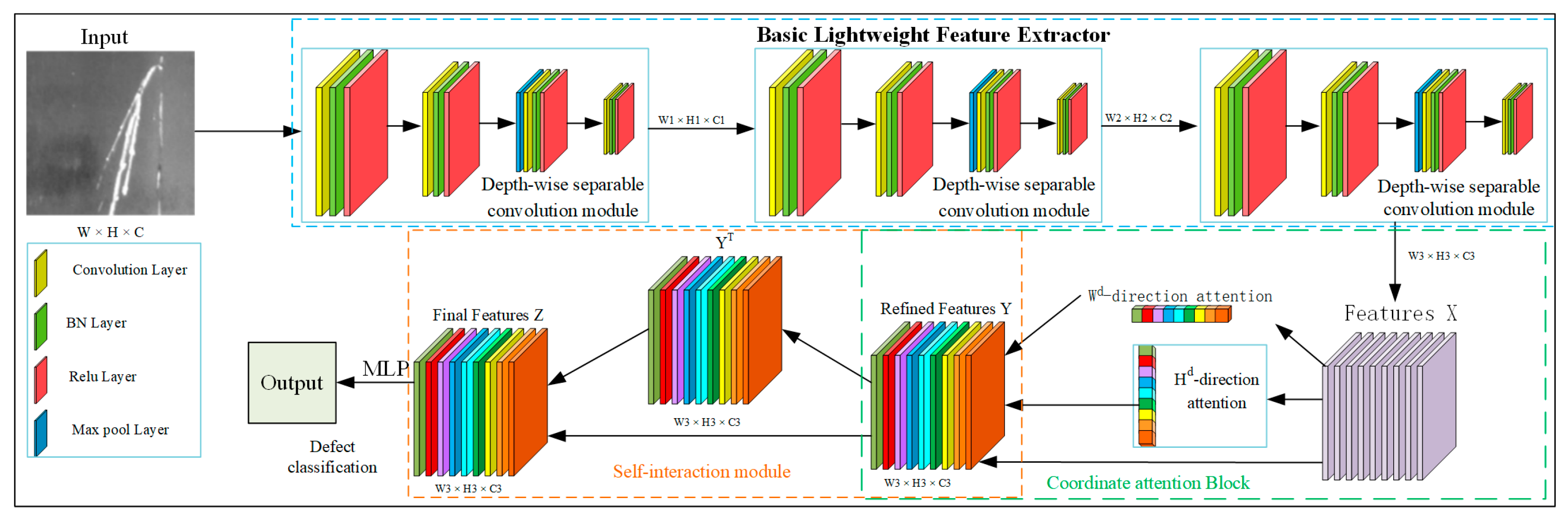
  85. Li, Z.; Wu, C.; Han, Q.; Hou, M.; Chen, G.; Weng, T. CASI-Net: A novel and effect steel surface defect classification method based on coordinate attention and self-interaction mechanism. Mathematics 2022, 10, 963. [Google Scholar] [CrossRef]
  86. Hinton, G.E.; Osindero, S.; Teh, Y.W. A fast learning algorithm for deep belief nets. Neural Comput. 2006, 18, 1527–1554. [Google Scholar] [CrossRef]
  87. Wang, X.B.; Li, J.; Yao, M.H.; He, W.X. Solar cells surface defects detection based on deep learning. Pattern Recognit. Artif. Intell. 2014, 27, 517–523. [Google Scholar]
  88. Shen, J.; Chen, P.; Su, L.; Shi, T.; Tang, Z.; Liao, G. X-ray inspection of TSV defects with self-organizing map network and Otsu algorithm. Microelectron. Reliab. 2016, 67, 129–134. [Google Scholar] [CrossRef]
  89. Liu, K.; Wang, H.; Chen, H.; Qu, E.; Tian, Y.; Sun, H. Steel surface defect detection using a new Haar-Weibull-variance model in unsupervised manner. IEEE Trans. Instrum. Meas. 2017, 66, 2585–2596. [Google Scholar] [CrossRef]
  90. Mei, S.; Yang, H. An unsupervised-learning-based approach for automated defect inspection on textured surfaces. IEEE Trans. Instrum. Meas. 2018, 67, 1266–1277. [Google Scholar] [CrossRef]
  91. Liu, K.; Li, A.; Wen, X.; Chen, H.; Yang, P. Steel surface defect detection using GAN and one-class classifier. In Proceedings of the 2019 25th International Conference on Automation and Computing (ICAC), Lancaster, UK, 5–7 September 2019; IEEE: Piscatevi, NJ, USA, 2019; pp. 1–6. [Google Scholar]
  92. Youkachen, S.; Ruchanurucks, M.; Phatrapomnant, T.; Kaneko, H. Defect segmentation of hot-rolled steel strip surface by using convolutional auto-encoder and conventional image processing. In Proceedings of the 2019 10th International Conference of Information and Communication Technology for Embedded Systems (IC-ICTES), Bangkok, Thailand, 25–27 March 2019; IEEE: Piscatevi, NJ, USA, 2019; pp. 1–5. [Google Scholar]
  93. Niu, M.; Song, K.; Huang, L.; Wang, Q.; Yan, Y.; Meng, Q. Unsupervised saliency detection of rail surface defects using stereoscopic images. IEEE Trans. Ind. Inform. 2021, 17, 2271–2281. [Google Scholar] [CrossRef]
  94. Zhou, Z.H. A brief introduction to weakly supervised learning. Natl. Sci. Rev. 2018, 5, 44–53. [Google Scholar] [CrossRef] [Green Version]
  95. Di, H.; Ke, X.; Peng, Z.; Dongdong, Z. Surface defect classification of steels with a new semi-supervised learning method. Opt. Lasers Eng. 2019, 117, 40–48. [Google Scholar] [CrossRef]
  96. Berthelot, D.; Carlini, N.; Goodfellow, I.; Papernot, N.; Oliver, A.; Raffel, C.A. Mixmatch: A holistic approach to semi-supervised learning. Adv. Neural Inf. Process. Syst. 2019, 32. [Google Scholar]
  97. He, Y.; Song, K.; Dong, H.; Yan, Y. Semi-supervised defect classification of steel surface based on multi-training and generative adversarial network. Opt. Lasers Eng. 2019, 122, 294–302. [Google Scholar] [CrossRef]
  98. Yun, J.P.; Shin, W.C.; Koo, G.; Kim, M.S.; Lee, C.; Lee, S.J. Automated defect inspection system for metal surfaces based on deep learning and data augmentation. J. Manuf. Syst. 2020, 55, 317–324. [Google Scholar] [CrossRef]
  99. Božič, J.; Tabernik, D.; Skočaj, D. Mixed supervision for surface-defect detection: From weakly to fully supervised learning. Comput. Ind. 2021, 129, 103459. [Google Scholar] [CrossRef]
  100. Tabernik, D.; Šela, S.; Skvarč, J.; Skočaj, D. Segmentation-based deep-learning approach for surface-defect detection. J. Intell. Manuf. 2020, 31, 759–776. [Google Scholar] [CrossRef] [Green Version]
  101. Božič, J.; Tabernik, D.; Skočaj, D. End-to-end training of a two-stage neural network for defect detection. In Proceedings of the 2020 25th International Conference on Pattern Recognition (ICPR), Milan, Italy, 10–15 January 2021; IEEE: Piscatevi, NJ, USA, 2021; pp. 5619–5626. [Google Scholar]
  102. Zhang, J.; Su, H.; Zou, W.; Gong, X.; Zhang, Z.; Shen, F. CADN: A weakly supervised learning-based category-aware object detection network for surface defect detection. Pattern Recognit. 2021, 109, 107571. [Google Scholar] [CrossRef]
  103. Li, J.; Su, Z.; Geng, J.; Yin, Y. Real-time detection of steel strip surface defects based on improved yolo detection network. IFAC-PapersOnLine 2018, 51, 76–81. [Google Scholar] [CrossRef]
  104. Yang, J.; Li, S.; Wang, Z.; Yang, G. Real-time tiny part defect detection system in manufacturing using deep learning. IEEE Access 2019, 7, 89278–89291. [Google Scholar] [CrossRef]
  105. Cheng, X.; Yu, J. RetinaNet with difference channel attention and adaptively spatial feature fusion for steel surface defect detection. IEEE Trans. Instrum. Meas. 2020, 70, 1–11. [Google Scholar] [CrossRef]
  106. Kou, X.; Liu, S.; Cheng, K.; Qian, Y. Development of a YOLO-V3-based model for detecting defects on steel strip surface. Measurement 2021, 182, 109454. [Google Scholar] [CrossRef]
  107. Chen, X.; Lv, J.; Fang, Y.; Du, S. Online Detection of Surface Defects Based on Improved YOLOV3. Sensors 2022, 22, 817. [Google Scholar] [CrossRef] [PubMed]
  108. Tian, R.; Jia, M. DCC-CenterNet: A rapid detection method for steel surface defects. Measurement 2022, 187, 110211. [Google Scholar] [CrossRef]
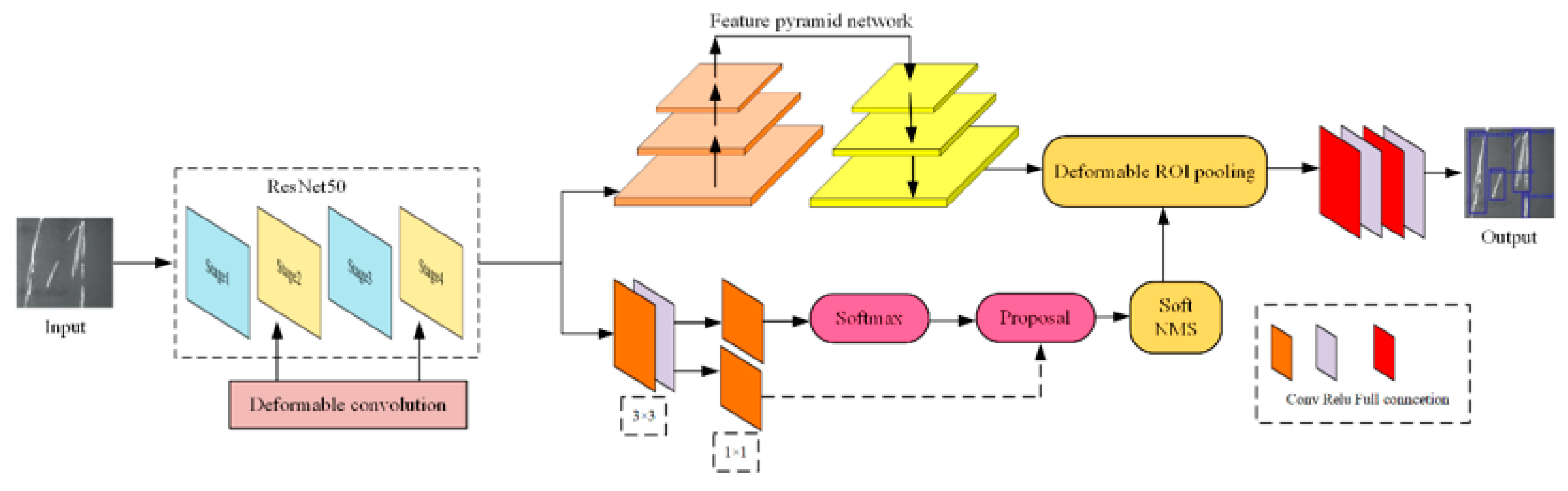
  109. Wei, R.; Song, Y.; Zhang, Y. Enhanced faster region convolutional neural networks for steel surface defect detection. ISIJ Int. 2020, 60, 539–545. [Google Scholar] [CrossRef] [Green Version]
  110. Zhao, W.; Chen, F.; Huang, H.; Li, D.; Cheng, W. A new steel defect detection algorithm based on deep learning. Comput. Intell. Neurosci. 2021, 2021. [Google Scholar] [CrossRef]
  111. Natarajan, V.; Hung, T.Y.; Vaikundam, S.; Chia, L.T. Convolutional networks for voting-based anomaly classification in metal surface inspection. In Proceedings of the 2017 IEEE International Conference on Industrial Technology (ICIT), Toronto, ON, Canada, 22–25 March 2017; IEEE: Piscatevi, NJ, USA, 2017; pp. 986–991. [Google Scholar]
  112. Ren, R.; Hung, T.; Tan, K.C. A generic deep-learning-based approach for automated surface inspection. IEEE Trans. Cybern. 2017, 48, 929–940. [Google Scholar] [CrossRef]
  113. Liu, Y.; Xu, K.; Xu, J. Periodic surface defect detection in steel plates based on deep learning. Appl. Sci. 2019, 9, 3127. [Google Scholar] [CrossRef] [Green Version]
  114. Song, L.; Lin, W.; Yang, Y.-G.; Zhu, X.; Guo, Q.; Xi, J. Weak micro-scratch detection based on deep convolutional neural network. IEEE Access 2019, 7, 27547–27554. [Google Scholar] [CrossRef]
  115. He, D.; Xu, K.; Wang, D. Design of multi-scale receptive field convolutional neural network for surface inspection of hot rolled steels. Image Vis. Comput. 2019, 89, 12–20. [Google Scholar] [CrossRef]
  116. Yang, H.; Chen, Y.; Song, K.; Yin, Z. Multiscale feature-clustering-based fully convolutional autoencoder for fast accurate visual inspection of texture surface defects. IEEE Trans. Autom. Sci. Eng. 2019, 16, 1450–1467. [Google Scholar] [CrossRef]
  117. Zhou, F.; Liu, G.; Ni, H.; Ren, F. A generic automated surface defect detection based on a bilinear model. Appl. Sci. 2019, 9, 3159. [Google Scholar] [CrossRef] [Green Version]
  118. Zhang, J.; Kang, X.; Ni, H.; Ren, F. Surface defect detection of steel strips based on classification priority YOLOv3-dense network. Ironmak. Steelmak. 2021, 48, 547–558. [Google Scholar] [CrossRef]
  119. Lin, C.Y.; Chen, C.H.; Yang, C.Y.; Akhyar, F.; Hsu, C.Y.; Ng, H.F. Cascading convolutional neural network for steel surface defect detection. In Proceedings of the International Conference on Applied Human Factors and Ergonomics, Washington, DC, USA , 24–28 July 2019; Springer: Cham, Switzerland, 2019; pp. 202–212. [Google Scholar]
  120. Song, K.; Yan, Y. Micro surface defect detection method for silicon steel strip based on saliency convex active contour model. Math. Probl. Eng. 2013, 2013, 1–13. [Google Scholar] [CrossRef]
  121. Buscema, M.; Terzi, S.; Tastle, W. A new meta-classifier. In Proceedings of the 2010 Annual Meeting of the North American Fuzzy Information Processing Society (NAFIPS), Toronto, ON, Canada, July 2010; pp. 1–7. [Google Scholar]
  122. Lv, X.; Duan, F.; Jiang, J.J.; Fu, X.; Gan, L. Deep metallic surface defect detection: The new benchmark and detection network. Sensors 2020, 20, 1562. [Google Scholar] [CrossRef] [Green Version]
  123. Gan, J.; Li, Q.; Wang, J.; Yu, H. A hierarchical extractor-based visual rail surface inspection system. IEEE Sens. J. 2017, 17, 7935–7944. [Google Scholar] [CrossRef]
  124. DAGM 2007 Datasets. Available online: https://hci.iwr.uni-heidelberg.de/node/3616 (accessed on 25 February 2021).
  125. Kylberg, G. The Kylberg Texture Dataset, V. 1.0. In Technical Report 35; Centre Image Anal., Swedish University of Agricultural Sciences: Uppsala, Sweden, 2011. [Google Scholar]
  126. Fan, D.P.; Cheng, M.M.; Liu, Y.; Li, T.; Borji, A. Structure-measure: A new way to evaluate foreground maps. In Proceedings of the IEEE International Conference on Computer Vision, Venice, Italy, 22–29 October 2017; pp. 4548–4557. [Google Scholar]
  127. Abdou, I.E.; Pratt, W.K. Quantitative design and evaluation of enhancement/thresholding edge detectors. Proc. IEEE 1979, 67, 753–763. [Google Scholar] [CrossRef]
  128. Tan, C.; Sun, F.; Kong, T.; Yang, C.; Liu, C. A survey on deep transfer learning. In International Conference on Artificial Neural Networks; Springer: Cham, Switzerland, 2018; pp. 270–279. [Google Scholar]
  129. Mujeeb, A.; Dai, W.; Erdt, M.; Sourin, A. Unsupervised surface defect detection using deep autoencoders and data augmentation. In Proceedings of the 2018 International Conference on Cyberworlds (CW), Singapore, 3–5 October 2018; IEEE: Piscatevi, NJ, USA, 2018; pp. 391–398. [Google Scholar]
  130. Niu, S.; Li, B.; Wang, X.; Lin, H. Defect image sample generation with GAN for improving defect recognition. IEEE Trans. Autom. Sci. Eng. 2020, 17, 1611–1622. [Google Scholar] [CrossRef]
  131. Schlegl, T.; Seebck, P.; Waldstein, S.M.; Langs, G.; Schmidt-Erfurth, U. f-AnoGAN: Fast unsupervised anomaly detection with generative adversarial networks. Med. Image Anal. 2019, 54, 30–44. [Google Scholar] [CrossRef] [PubMed]
  132. Li, M.; Xiong, A.; Wang, L.; Deng, S.; Ye, J. ACO Resampling: Enhancing the performance of oversampling methods for class imbalance classification. Knowl.-Based Syst. 2020, 196, 105818. [Google Scholar] [CrossRef]
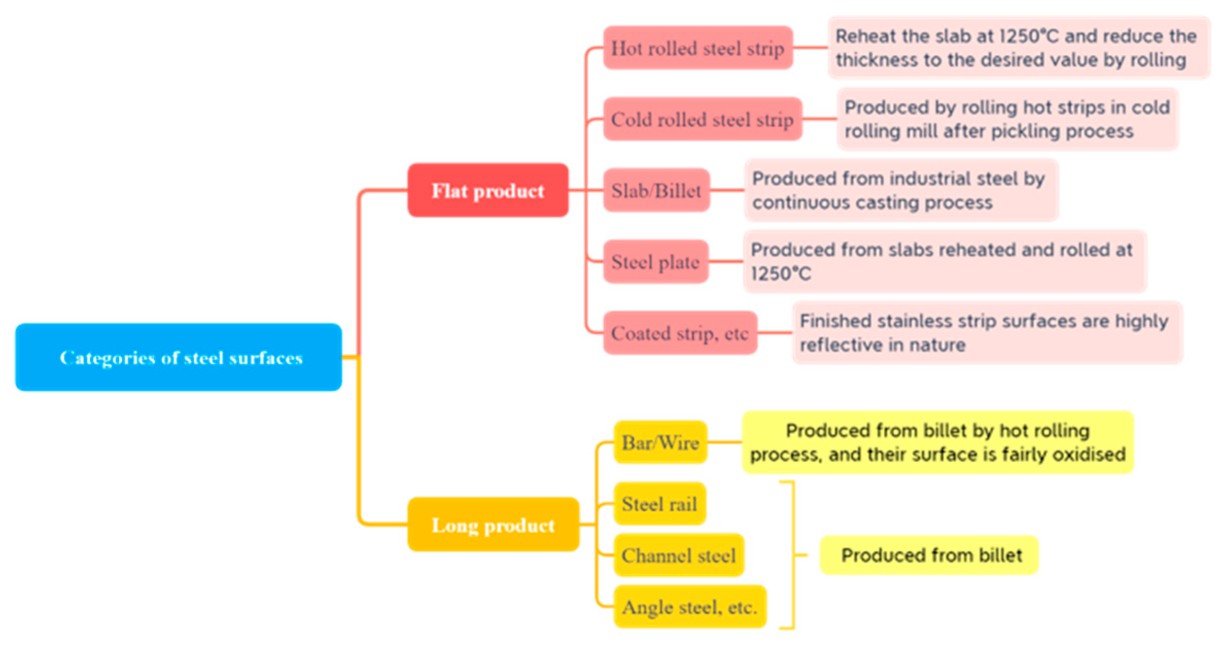
Figure 1. Categories of steel products.
Coatings 13 00017 g001
Figure 2. Development process of technologies related to industrial surface defect detection. Viola Jones [13], HOG [14], DPM [15], AlexNet [16], GAN [17], VGG [18], Google [19], SPPNet [20], RCNN [21], ResNet [22], Fast RCNN [23], SSD [24], SqueezeNet [25], Faster RCNN [26], YOLO [27], RetinaNet [28], Cascade RCNN [29], DenseNet [30], MobileNet [31], ShuffleNet [32], CenterNet [33].
Coatings 13 00017 g002
Figure 3. Steel surface defect recognition system.
Coatings 13 00017 g003
Figure 4. Classification of traditional machine learning methods.
Coatings 13 00017 g004
Figure 5. Defect recognition algorithm based on deep learning.
Coatings 13 00017 g005
Figure 6. Model outline diagram [35].
Coatings 13 00017 g006
Figure 7. Overview of the CASI-Net framework [85].
Coatings 13 00017 g007
Figure 8. Diagram of the outline of the deep learning methods.
Coatings 13 00017 g008
Figure 9. The improved method of Faster R-CNN [110].
Coatings 13 00017 g009
Figure 10. Calculation of PRE and RECALL in the object detection algorithm.
Coatings 13 00017 g010
Table 1. Statistics of the steel surface defect categories.
Steel Surface TypeDefect Category
SlabCrack, pitting, scratches, scarfing defect
PlateCrack, scratch, seam
BilletCorner crack, line defect, scratch
Hot rolled steel stripHole, scratch, rolled in scale, crack, pits/scab, edge defect/coil break, shell, lamination, sliver
Cold rolled steel stripLamination, roll mark, hole, oil spot, fold, dark, heat buckle, inclusion, rust, sliver, scale, scratch, edge etc.
Stainless steelHole, scale, scratch, inclusion, roll mark, shell, blowhole
Wire/BarSpot, dark line, seam, crack, lap, overfill, scratch etc.
Table 2. Summary of algorithms based on image texture features.
CategoryYearRef.ObjectFunctionMethodsPerformance
Statistical Based Methods2013[45]Hot rolled steel stripDefect ClassificationLocal binary patternSNR = 40, ACC = 0.9893
2014[46]Steel stripDefect ClassificationCo-occurrence matrixACC = 0.9600
2015[47]Steel stripDefect ClassificationLocal binary patternACC = 0.9005
2017[48]Steel stripDefect LocationAuto threshold-
2017[49]Hot rolled steel stripDefect ClassificationLocal binary patternACC = 0.9762, FPS = 10
2017[50]SteelDefect ClassificationHistogram, co-occurrence matrixACC = 0.9091
2018[51]SteelDefect ClassificationLocal descriptorsACC = 0.9982, FPS = 38.4
2018[52]Hot rolled steel stripDefect ClassificationLocal binary patternTPR = 0.9856, FPR = 0.2900, FPS = 11.08
2019[53]Plate steelDefect ClassificationLocal binary mode, gray histogramACC = 0.9440, FPS = 15.87
Filter Based Methods2012[54]Hot rolled steel stripDefect ClassificationCurved wave transformACC = 0.9733
2015[55]Thick steel plateDefect DetectionGaborACC = 0.9670, FPR = 0.75
2015[56]Continuous casting slabsDefect ClassificationShearletACC = 0.9420
2017[57]Steel slabsDefect DetectionGaborACC = 0.9841
2018[58]Hot rolled steel stripDefect ClassificationShearletACC = 0.9600
2013[59]Hot rolled steel stripDefect DetectionWavelet transformG-mean = 0.9380, Fm = 0.9040
2014[60]Plate steelDefect DetectionGaborTPR = 0.9446, FNR = 0.29
2019[61]Continuous casting slabsDefect ClassificationContour waveAP = 0.9787
Structure Based Methods2016[41]Steel railsDefect LocationEdge-
2010[62]Steel stripDefect LocationEdge-
2015[63]Steel stripDefect DetectionMorphological operationsME = 0.0818, EMM = 0.3100, RAE = 0.0834
2016[64]Steel railsDefect LocationSkeletonACC = 0.9473, FPS = 1.64
2014[65]Silicon SteelDefect SegmentationMorphological operations-
Model Based Methods2018[66]Steel stripDefect SegmentationGuidance templatePRE = 0.9520, RECALL = 0.9730, Fm = 0.9620, FPS = 28.57
2018[67]Steel sheetDefect SegmentationLow-rank matrix modelAUC = 0.835, Fm = 0.6060, MAE = 0.1580, FPS = 5.848
2019[68]High strength steel jointsDefect ClassificationFractal modelACC = 0.8833
2013[69]Steel stripDefect SegmentationMarkov modelCSR = 0.9440, WSR = 0.1880
2019[70]Hot rolled steelDefect SegmentationCompact modelFPR = 0.088, FNR = 0.2660, MAE = 0.1430
* SNR indicates Gaussian noise, ME indicates misclassification error, EMM indicates edge mismatch, RAE indicates relative foreground area error, CSR indicates correct segmentation rate, WSR indicates wrong segmentation rate, FNR indicates false negative rate, FPR indicates false positive rate, MAE indicates mean square error, AUC indicates area under the curve, TPR indicates true positive rate, FPS indicates frames per second.
Table 3. Summary of methods based on the image texture features.
CategoryMethodsRef.AdvantagesDisadvantages
Statistical Based MethodsThreshold technology[48]Simple, easy to understand and implement.It is difficult to detect defects that do not differ much from the background.
Clustering[49]Strong anti-noise ability and high computational efficiencyVulnerable to pseudo defect interference.
Grayscale feature statistics[50]Suitable for processing low resolution images.Low timeliness, no automatic threshold selection.
Co-occurrence matrix[46]The extracted image pixel space relationship is complete and accurate.The computational complexity and memory requirements are relatively high.
Local binary pattern[47]Discriminative features with rotation and gray scale invariance can be extracted quickly.Weak noise immunity, pseudo-defect interference.
Histogram[53]Suitable for processing images with a large grayscale gap between the defect and the background.Low detection efficiency for complex backgrounds, or images with defects similar to the background.
Filter Based MethodsGabor filter[55]Suitable for high-dimensional feature spaces with low computational burden.Difficult to determine optimal filter parameters and no rotational invariance.
Wavelet filters[59]Suitable for multi-scale image analysis, which can effectively compress images with less information loss.Vulnerable to correlation of features between scales.
Multi-scale geometric analysis[56]Optimal sparse representation for high-dimensional data, capable of handling images with strong noise background.The problem of feature redundancy exists.
Curvelet transform[54]High anisotropy with good ability to express information along the edges of the graph.Complex to implement and less efficient.
Shearlet and its variants[58]Multi-scale decomposition and the ability to efficiently capture anisotropic features.Difficult to retain original image detail information.
Structure Based MethodsEdge[41]It is suitable for extracting some low-order features of the image and is easy to implement.Vulnerable to noise and only suitable for low resolution images.
Skeleton[64]Almost distortion less representation of the geometric and topological properties of objects.Unsatisfactory image processing for complex backgrounds.
Morphological operations[63]Great for random or natural textures, easy to calculate.Only for non-periodic image defects.
Model Based MethodsGaussian mixture model[66]Correlation between features can be captured automatically.Large computational volume and slow convergence, sensitive to outliers.
Fractal model[68]The overall information of an image can be represented by partial features.Unsatisfactory detection accuracy and limitation for images without self-similarity.
Low-rank matrix model[67]Strong discriminatory ability and adaptive nearest neighbor.Unsatisfactory detection accuracy.
MRF model[69]Can combine statistical and spectral methods for segmentation applications to capture local texture orientation information.Cannot detect small defects. Not applicable to global texture analysis.
Table 4. Summary of the features of deep learning methods.
CategoryAdvantagesDisadvantages
Supervised methodsHigh precision, good adaptability, wide range of applications.Dataset annotation is heavy and difficult to make.
Unsupervised methodsIt can be trained directly using label-free data with simple techniques.Relatively low precision, unstable training results are easily affected by noise and initial parameters.
Weakly supervised methodsIt has the advantages of both supervised and unsupervised methods.The training process is tedious and the technical implementation is complicated.
Table 5. Summary of deep learning-based algorithms.
CategoryYearRef.MethodsObjectFunctionPerformance
Supervised Methods2017[111]CNNMetalDefect ClassificationACC = 0.9207
2017[112]DecayMulti-TypeDefect DetectionACC = 0.9400, FPS = 17, EE = 0.2100
2019[113]VGG + LSTMSteel plateDefect DetectionACC = 0.8620
2019[114]Du-NetMetalDefect SegmentationACC = 0.8345
2019[115]InceptionV4Hot rolled SteelDefect ClassificationRR = 0.9710
2019[79]SqueezeNetSteelDefect ClassificationACC = 0.9750, FPS = 100, Model size = 3.1 MB
2019[80]MG-CNNHot rolled SteelDefect classification and LocationCR = 0.9830, DR = 0.9600
2020[81]ResNet50SteelDefect ClassificationPRE = 0.8160, ACC = 0.9670, F1 = 0.6610, RECALL = 0.5670
2021[82]DA-ACNNSteelDefect ClassificationACC = 0.9900
2021[83]RepVGGHot rolled steel stripDefect ClassificationACC = 0.9510, RCALL = 0.9392, PRE = 0.9516, F1 = 0.9325, Params = 83.825 M
2021[4]Unet + XceptionRolled pieceDefect Classification and SegmentationPRE = 0.8400, RECALL = 0.9000, Dice score = 0.5950
2021[35]VGG19Steel stripDefect ClassificationACC = 0.9762, FPS = 52.1
2021[37]DAN-DeepLabv3+SteelDefect Precise SegmentationmIoU = 0.8537, PRE = 0.9544, RECALL = 0.9071, F1 = 0.9297
2021[84]ResNet34Steel stripDefect Precise Seg-mentationMAE = 0.0125, WF = 0.9200, OR = 0.8380, SM = 0.9380, PFOM = 0.9120, FPS = 47.6
2022[85]CASI-NetHot rolled steel stripDefect ClassificationACC = 0.9583, Params = 2.22 M
Unsupervised Methods2020[93]GLRNNRSteel railsDefect Detection and SegmentationMAE = 0.0900, AUC = 0.9400, PRE = 0.9481, RECALL = 0.8066, Fm = 0.8716
2017[90]MSCDAEMulti-TypeDefect Detection and SegmentationRECALL = 0.6440, PRE = 0.6400, FA = 0.6380
2019[92]CAEHot rolled steel stripDefect Segmentation--
2018[116]FCAEMulti-TypeDefect SegmentationPRE = 0.9200, FPS = 12.2
2019[91]GANSteel stripDefect DetectionPRE = 0.9410, RECALL = 0.9380, Fm = 0.9390
2017[89]HWVSteelDefect SegmentationFPS = 19.23, PRE = 0.9570, RECALL = 0.9680, Fm = 0.9620
Weakly Supervised Methods2019[40]GANMulti-TypeDefect Classification and SegmentationRECALL = 0.8710, ACC = 0.9920, AUC = 0.9140
2019[95]CAE + GANSteelDefect ClassificationCR = 0.9650
2019[117]D-VGG16Multi-TypeDefect Classification and SegmentationAP = 0.9913, PR = 0.9836, TPR = 0.9967, FPR = 0.0164, FNR = 0.0033
2019[97]GAN + ResNet18SteelDefect ClassificationACC = 0.9507
2020[102]CANDMulti-TypeDefect Classification and SegmentationACC = 0.8910, PRE = 0.5510, RECALL = 0.9200, F1 = 0.6900, mAP = 0.6120
2020[98]CVAEMetalDefect ClassificationACC = 0.9969, F1 = 0.9971
2021[99]Dual network modelSteelDefect Classification and SegmentationAP = 0.9573
Single-stage Methods2018[103]YOLOSteel stripDefect Classification and LocationACC = 0.9755, FPS = 83, mAP = 0.9755, RECALL = 0.9586
2020[118]YOLOV3-DenseSteel stripDefect Classification and LocationmAP = 0.8273, FPS = 103.3, F1 = 0.8390
2021[105]RetinaNetSteelDefect Classification and LocationmAP = 0.7825, FPS = 12, FLOPs = 105.3, Params = 42.2
2021[106]YOLOV3Steel stripDefect Classification and LocationmAP = 0.7220, FPS = 64.5
2022[107]YOLOV3Hot rolled steel stripDefect Classification and LocationPRE = 0.9837, RECALL = 0.9548, F1 = 0.9690, mAP = 0.8696, FPS = 80.96
2022[108]Center
Net
SteelDefect Classification and LocationmAP = 0.7941, FPS = 71.37
Two-stage Methods2020[119]SSD + ResnetSteelDefect Classification and LocationPRE = 0.9714, RECALL = 0.9214, Fm = 0.9449
2020[109]Faster RCNNSteelDefect Classification and LocationDR = 0.9700, FDR = 0.1680
2021[36]Faster RCNNSteelDefect Classification and LocationACC = 0.9820, FPS = 15.9, F1 = 0.9752
2021[110]Faster RCNN + FPNSteelDefect Classification and LocationmAP = 0.7520
2022[8]YOLOV5 + Optimized-Inception-ResNetV2Hot rolled steel stripDefect Classification and LocationmAP = 0.8133, FPS = 24, Param = 37.7, RECALL = 0.7630
* RR indicates recognition rates, CR indicates classification rate, DR indicates detection rate, OR indicates overlapping ratio, FDR indicates false detection rate.
Table 6. Summary of the datasets.
DatasetObjectDescriptionLink
NEU [45]Hot rolled steel strip1800 grayscale images of hot-rolled strip containing six types of defects, 300 samples of each.http://faculty.neu.edu.cn/songkc/en/zdylm/263265 (accessed on 9 November 2022)
Micro Surface Defect Database [120]Hot rolled steel stripMicrominiature strip defect data, with defects only about 6 × 6 pixels in size.http://faculty.neu.edu.cn/songkc/en/zdylm/263266 (accessed on 9 November 2022)
X-SSD [83]Hot rolled steel strip7 typical defects of hot-rolled steel strip, with 1360 defect images.https://github.com/Fighter20092392/X-SDD-A-New-benchmark (accessed on 9 November 2022)
Oil Pollution Defect Database [65]Silicon SteelOil-disturbed silicon steel surface defects datasethttp://faculty.neu.edu.cn/songkc/en/zdylm/263267 (accessed on 9 November 2022)
Severstal: Steel Defect DetectionSteel plateThere are 12,568 grayscale images of steel plates of size 1600 × 256 in the training dataset, and the images are divided into 4 categories.https://www.kaggle.com/c/severstal-steel-defect-detection/data (accessed on 9 November 2022)
UCI Steel Plates Faults Data Set [121]Steel stripThis dataset contains 7 types of strip defects. This dataset is not image data, but data of 28 features of strip defects.https://archive-beta.ics.uci.edu/dataset/198/steel+plates+faults (accessed on 2 May 2022)
SD-saliencySteel stripContains a total of 900 cropped images containing 3 types of defects, each with a resolution of 200 × 200.https://github.com/SongGuorong/MCITF/tree/master/SD-saliency-900 (accessed on 9 November 2022)
GC10-DET [122]Steel stripThe dataset contains 2257 images of steel strip with 10 defect types and an image resolution of 4096 × 1000https://github.com/lvxiaoming2019/GC10-DET-Metallic-Surface-Defect-Datasets (accessed on 2 May 2022)
RSDDs Dataset [123]Steel railsTwo types of orbital surface images (67 images and 128 images)http://icn.bjtu.edu.cn/Visint/resources/RSDDs.aspx (accessed on 2 May 2022)
DAGM [124]Multi-TypeIncludes 10 different computer-generated grayscale images of surfaces containing various defects.https://hci.iwr.uni-heidelberg.de/node/3616 (accessed on 2 May 2022)
KolektorSSD2 [99]Multi-TypeThis dataset training set test set contains a total of 3335 color images, more than 5 kinds of defects.https://www.vicos.si/resources/kolektorsdd2/ (accessed on 2 May 2022)
Kylberg Texture Dataset [125]Multi-TypeThe dataset contains 28 texture classes, each with 160 unique texture patches.http://www.cb.uu.se/~gustaf/texture/ (accessed on 2 May 2022)
Disclaimer/Publisher’s Note: The statements, opinions and data contained in all publications are solely those of the individual author(s) and contributor(s) and not of MDPI and/or the editor(s). MDPI and/or the editor(s) disclaim responsibility for any injury to people or property resulting from any ideas, methods, instructions or products referred to in the content.

