Multi-Scale Lightweight Neural Network for Steel Surface Defect Detection

Abstract

Defect classification is an important aspect of steel surface defect detection. Traditional approaches for steel surface defect classification employ convolutional neural networks (CNNs) to improve accuracy, typically by increasing network depth and parameter count. However, this approach overlooks the significant memory overhead of large models, and the incremental gains in accuracy diminish as the number of parameters increases. To address these issues, a multi-scale lightweight neural network model (MM) is proposed. The MM model, with a fusion encoding module as its core, constructs a multi-scale neural network by utilizing the Gaussian difference pyramid. This approach enhances the network’s ability to capture patterns at different resolutions while achieving superior model accuracy and efficiency. Experimental results on a dataset from a hot-rolled strip steel plant demonstrate that the MM network achieves a classification accuracy of 98.06% in defect classification tasks. Compared to networks such as ResNet-50, ResNet-101, VGG, AlexNet, MobileNetV2, and MobileNetV3, the MM model not only reduces the number of model parameters and compresses model size but also achieves better classification accuracy.

1. Introduction

Defect classification is an important industrial inspection task where defect images are analyzed and identified to determine their corresponding defect types [1]. Manual defect detection is commonly used to classify steel surface defects in traditional industries. It is an essential component of the industrial defect detection process. To replace manual operations, it is desired that machines can automatically detect steel surface defects using computer vision technology [2].

The task of classifying defects on steel surfaces using computer vision techniques poses a significant challenge due to the effects of illumination and material variations on defect images [3]. In addition, the appearance of defects varies dramatically not only within categories of steel surfaces but also between categories, thus further complicating the classification process. Therefore, designing an accurate and reliable defect classification algorithm to take these complexities into account is an ongoing research topic in the field of computer vision [4]. Current image classification methods are mainly of two types: traditional machine learning image classification algorithms and deep learning methods based on convolutional neural networks [5]. Traditional image classification algorithms are mainly implemented using two major steps of feature extraction and classifier design, such as the K-Nearest Neighbor algorithm [6], Support Vector Machine [7], and neural networks [8], which are widely used in computer vision. Various complex situations are faced in practical defect classification applications, and it is difficult to achieve the requirements in terms of accuracy using traditional image processing methods [9].

The identification of surface defects in steel undergoes three processes: manual human detection, prediction using machine learning algorithms, and automatic detection through deep learning [10]. In recent years, deep learning-based image classification methods have achieved good results, such as VGGNet (Visual Geometry Group Network) [11] and ResNet (Residual Network) [12]. U-Net is employed for the task of detecting and classifying welding defects using X-ray images, artificial neural networks, and image analysis methods [13,14]. We introduced a novel deep learning-based approach for detecting and classifying surface defects that occur during the steel production process. This method enhances classification performance through parallel training of residual and attention structures. LSHADE-SVC-PCD proposes an intelligent method for automatic detection of pitting corrosion by employing LSHADE metaheuristics, SVM machine learning, and image processing techniques [15,16]. We proposed a defect detection algorithm based on deformable networks combined with a multi-scale feature fusion algorithm leveraging a deformable convolutional neural network. However, state-of-the-art CNNs require billions of floating-point operations, which makes them unusable for mobile or embedded devices. For example, ResNet-101 has a complexity of 7.8 × 10⁹ FLOPs (floating-point operations per second), which makes real-time detection impossible even with powerful GPUs. Considering the huge computational cost of modern CNNs, lightweight neural networks have been proposed to be deployed on mobile or embedded devices. For example, MobileNetV1 [17] and MobileNetV2 [18] use depth-separable convolution to build lightweight networks. ShuffleNet [19] uses grouped convolution and depth-separable convolution to build lightweight networks. SqueezeNet [20] uses the core module Fire to compress the model parameters, reduce the depth of the network, and decrease the size of the model. SENet (Squeeze-and-Excitation Network) [21] proposes the SE module as a lightweight attention mechanism to adaptively calibrate the feature map by learning the channel importance; however, the SE module only focuses on the influence of the channel aspect of the feature map and ignores the importance of the spatial dimension.

Lightweight networks [22] can achieve relatively high accuracy with limited computational budgets. However, existing lightweight networks tend to use “sparsely connected” convolution, such as deep convolution and group convolution, rather than the standard “fully connected” convolution. This “sparsely connected” convolution, while reducing the number of parameters, can to some extent hinder the exchange of information between groups, resulting in a degradation of network performance. Since a practical steel defect classification algorithm needs to be deployed on CPUs or even embedded systems, an algorithm with low computational complexity and high classification accuracy that can avoid intergroup information loss is needed.

In this paper, a novel multiscale neural network model (MM) is proposed to build a multiscale neural network model with a fusion coding module as the core and a Gaussian difference pyramid to obtain better model accuracy and efficiency while improving the network’s ability to capture patterns of different resolutions. The feasibility and effectiveness of the model and method are verified through experiments on the surface defect detection of steel sheet products in a factory. By comparing the results with other methods, it can be concluded that the multiscale neural network model avoids the loss of information between groups, further reduces the number of parameters and computational effort, and significantly improves classification accuracy.

Our main contributions can be summarized as follows:

(1)

We propose a method that utilizes the Gaussian difference pyramid to construct a scale space by iteratively building a pyramid structure at different scales and effectively detecting key points in images through a scale-invariant feature transform.

(2)

We employ the multi-kernel fusion approach to capture both blurred and fine-grained features at different resolutions, enhancing the accuracy and efficiency of the model.

(3)

By integrating the fusion encoding and matching transformation of keypoints with the original network, we address the challenges of exchanging information, avoiding information loss, and improving performance in multi-scale space.

(4)

The proposed Multi-Scale Lightweight Neural Network (MM) achieves better classification accuracy while reducing model parameters and compressing model size.

The structure of this paper is as follows: Section 1 presents an overview of the proposed model’s overall structure. Section 2 discusses the method employed to address the overfitting issue. In Section 3, the dataset and evaluation of the proposed model are presented in detail, followed by a discussion of the results. Finally, Section 4 concludes the paper.

2. Construction of a Multi-Scale Neural Network Model

The problem of compression and acceleration of neural networks has become a hot research topic in the field of deep learning due to the large computational volume and model capacity of deep neural networks. As the demand for high-quality deep neural networks running on embedded devices increases, researchers are exploring the design of lightweight network models to reduce computational costs. These models often use “sparsely connected” convolutions, which can lower computational demands but may also inhibit information exchange between different groups within the network. In this paper, we propose a multiscale neural network by borrowing the idea of the Gaussian difference pyramid [23] and adding a fusion coding module [24]. The network improves classification accuracy while decreasing the computational cost.

2.1. Constructing Key-Point Feature Sets Based on Scale Space

In the steel slice dataset, the representation of images is represented at multiple scales. To effectively capture these features at different scales, we propose a method to construct the scale space using Gaussian [25] difference pyramids. In the scale space construction module, we construct the scale space by Gaussian blurring the image and calculating the difference between adjacent Gaussian blurred images. This process is iterated over different scales (i.e., the size or resolution of the image), forming a kind of pyramid structure. In this structure, each layer of the image is more blurred compared to the previous layer, and the resolution is reduced accordingly. By using this scale-space building block, we are able to effectively detect key points in the image during the scale-invariant feature transform (SIFT).

Gaussian differential pyramids provide an effective scale-space representation that captures the features of an image at different scales [26]. This is important for dealing with real-world image problems, as real-world objects can appear at a variety of different scales. In addition, the Gaussian difference pyramid offers the advantage of precise localization of feature points in images and provides multi-scale image information for analysis and processing. Furthermore, the downsampling of images in the pyramid reduces computational complexity, thereby enhancing computational efficiency. These characteristics make the Gaussian difference pyramid widely utilized in the fields of image processing, computer vision, and pattern recognition.

2.2. Convolution of Key-Point Features

The traditional convolutional layer in convolutional neural networks (CNNs) preserves global spatial information during the convolution process but may overlook crucial details. Due to the lack of explicit focus on key points, traditional convolutional layers may not be as effective as key-point feature convolution in extracting important features. Additionally, traditional convolutional layers do not specifically handle key points, leading to a lower sensitivity for accurately capturing significant key points in images. This limitation can restrict the performance of models on tasks related to key points. Key-point feature convolution is a group convolution of each key-point feature set into a separate set, which reduces the number of parameters and computational cost [27]. Using the idea of multi-core combination, convolution using different key point feature sets can enhance the model’s ability to adapt to varying levels of detail. The network needs both fuzzy key-point features to capture high-resolution patterns and fine key-point features to capture low-resolution patterns for better model accuracy and efficiency.

2.3. Key-Point Feature Set Mapping Fusion Module

The key-point feature set mapping fusion module has an advantage over traditional convolutional layers in convolutional neural networks (CNNs) as it explicitly focuses on key points and integrates their important information into the network, thereby enhancing the perception and utilization of crucial details in images and improving the robustness and accuracy of the model. On the other hand, traditional convolutional layers exhibit drawbacks in handling key details and tasks related to key points, such as disregarding fine details, a limited receptive field, and a lack of explicit attention to key points. To address issues related to information exchange, loss, and performance degradation of key-point features in multi-scale space [28], The paper suggests using key points to map and encode information from different scales, then combining it with the original network through matching transformations in order to enhance the discriminative features.

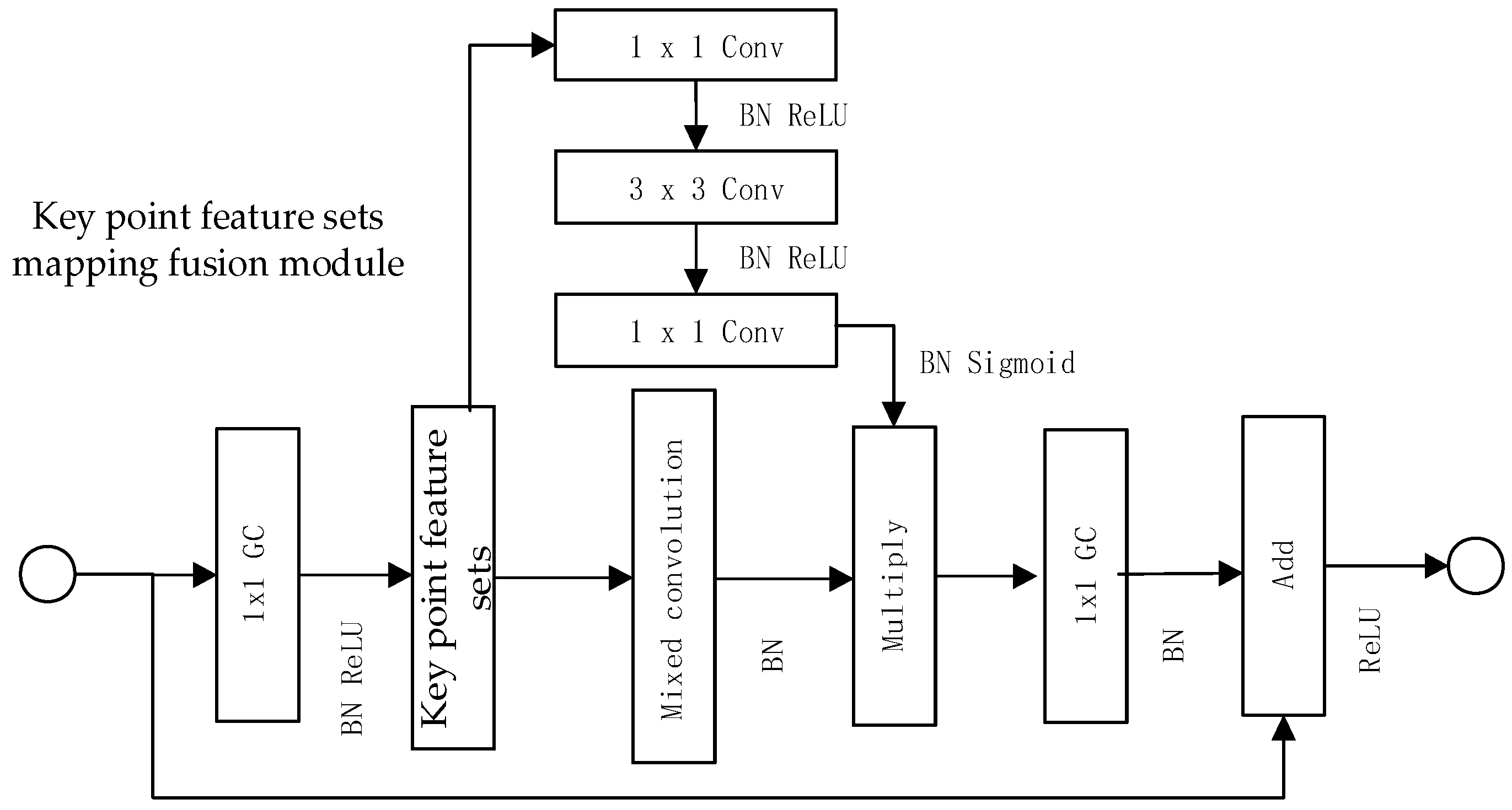
Key-point feature mapping fusion aims to combine essential feature points and incorporate information about their varying scales in order to create a comprehensive feature map, the process is shown in Figure 1. On top of the original feature map F ∈ RC × H × W generated by the Gaussian difference pyramid, the fusion module performs the fusion encoding transformation TF: RC × H × W → RCM × H × W to achieve the purpose of aggregating all key-point features. Where: C is the key-point feature of the original feature map; H and W are the width and height of the original feature map; CM is the key-point feature of the fused feature map.

The image is decomposed by a Gaussian differential pyramid to produce N different resolution images, and the Gaussian differential pyramid consists of multiple groups of pyramids, where each group of pyramids contains several layers, and the Gaussian differential pyramid consists of layer orders constructed on the basis of the Gaussian pyramid [29]. The process of decomposing a Gaussian image into its differential pyramid involves:

Step 1. Initialize i = 0;

Step 2. Standard image I(x,y) is sampled to obtain the first layer of the first set of Gaussian pyramid images g_0,0;

Step 3. Initialize j = 0 and x = 0;

Step 4. The Gaussian kernel Gx is convolved with image g_i,0 [30]:

$$G_x\left(x,y,{\sigma }_x\right)=\frac{1}{2\pi {\sigma }_x^2}{e}^{\frac{{\left(x-x_0\right)}^2+{\left(y-y_0\right)}^2}{2{\sigma }_x{}^2}}$$

(1)

$$g_{i,j+1}(x,y)=g_{i,j}(x,y)\otimes G_x\left(x,y,{\sigma }_x\right)$$

(2)

where ${\sigma }_x$ is the smoothing parameter.

Step 5. Differentiate the Gaussian image from the Gaussian image to obtain the Gaussian difference image [31]:

$$d_{i,x}(x,y)=g_{i,j}(x,y)-g_{i,j+1}(x,y)$$

(3)

Step 6. j = j + 1 and x = x + 1, iterate Steps 4 and 5, and when j > n − 1 and x > n − 2, perform Step 7;

Step 7. Downsample the image to get the Gaussian image of layer i + 1. When i = I + 1, go to Step 3, and the decomposition process ends when i > m − 1 is satisfied.

2.4. MM Network Construction

Based on Section 2.1 “Constructing Key-Point Feature Sets Based on Scale Space”, Section 2.2 “Convolution of Key-Point Features” and Section 2.3 “Key-Point Feature Set Mapping Fusion Module”, the MM network is proposed in this paper. The MM network is shown in Figure 2. The network consists of three branches from bottom to top: the standard branch, the dimension reduction branch, and the fusion branch. The standard branch directly maps the original feature map. The dimension reduction branch reduces computational costs and then performs Section 2.1 “Constructing Key-Point Feature Sets Based on Scale Space” operations to construct a set of key-point features. The fusion branch utilizes mixed convolutional kernels to obtain more stable feature maps at different resolutions, where the large convolutional kernel in the mixed convolution retains more feature information. It serves as a bridge connecting the dimension reduction branch and the fusion branch by combining the processed feature maps from the fusion branch. The final single-point group convolution is used to restore the channel dimension to match the standard branch. The fusion branch performs fusion encoding on the network and combines with the dimension reduction branch using element-wise multiplication before the single-point group convolution, which helps to reduce the loss of inter-group information during the convolution process. In this figure, “GC” represents Group Convolution, “Conv” represents Convolution, and “BN” represents Batch Normalization.

3. Solving the Overfitting Problem

To avoid overfitting problems, We perform batch normalization of the network as well as Dropout operations on the last two fully connected layers of the network [32]. Unlike L1 and L2 normalization, Dropout does not rely on the modification of the cost function; in Dropout, the network itself is changed. Assuming training data x and a corresponding target output y, the contribution to the gradient is normally determined by forward propagating x in the network and then back-propagating. However, using the Dropout operation, this paper starts by randomly removing half of the hidden neurons in the network while leaving the neurons in the input and output layers unchanged, after which the input x is forward propagated and the contribution to the gradient is determined by modifying the network, back-propagating the result, and repeating the process. The overall execution process is: first reset the neurons of Dropout; then select a new random subset of hidden neurons for deletion; and finally, update the weights and biases by estimating the gradient for a different small batch of data before determining.

Batch normalization is a normalization technique applied in hidden layers that normalizes the inputs of each layer by subtracting the batch mean and dividing by the batch standard deviation. This normalization process helps stabilize the distribution of activation values in the network, reducing the range of gradient variations, thereby accelerating training and improving the generalization ability of the network.

In practice, batch normalization not only improves training effectiveness but also has a certain regularization effect. By introducing randomness in each batch, it reduces reliance on dropouts. This is because the introduced randomness in batch normalization reduces the dependence of the network on individual neurons, thus reducing the risk of overfitting. Therefore, in networks with batch normalization, lower dropout rates can typically be used, or dropout operations may not be necessary at all.

Batch normalization plays a significant role in reducing dropout rates. By standardizing the inputs and stabilizing the distribution of activation values in the network, the reliance on Dropout operations is alleviated. This allows for a better balance between model capacity and the risk of overfitting, thereby improving the generalization ability and training effectiveness of the model.

4. Experiment

This section first describes the system that utilizes a CCD camera to capture images of the surface of hot-rolled steel strips, which are then subjected to normalization pre-processing. A sliding window approach is employed to extract image patches, which are used to construct a dataset of standard defect images. The dataset consists of six defect categories, including transverse cracks, wrinkles, longitudinal cracks, edge cracks, seams, and water stains. The training and validation of the system are performed using a multi-scale lightweight neural network model, and the performance of the model is evaluated and analyzed. Experimental results demonstrate that the proposed model achieves high accuracy and efficiency in detecting surface defects in hot-rolled steel strips. Compared to other classical and lightweight neural network models, the proposed model exhibits superior capability in detecting minor defects with high classification accuracy and performance.

4.1. Common Defects and Detection Process

The defect images are acquired based on a machine vision technology acquisition system, using a system consisting of CCD cameras as well as a deep neural network server. The images of the hot rolled strip surface are obtained through CCD cameras, and then the image data are received and transmitted to process the defect images of the hot rolled strip surface obtained within the cameras. The defect images are acquired based on a machine vision technology acquisition system, using a system consisting of CCD cameras as well as a deep neural network server. The images of the hot rolled strip surface are obtained through CCD cameras, and then the image data are received and transmitted to process the defect images of the hot rolled strip surface obtained within the cameras [33]. The data sets used in this paper are obtained through such image acquisition units, taken from a hot-rolled strip mill specializing in the production of cover hot-rolled strip surfaces, with more than 20,000 original sample images taken from different production batches.

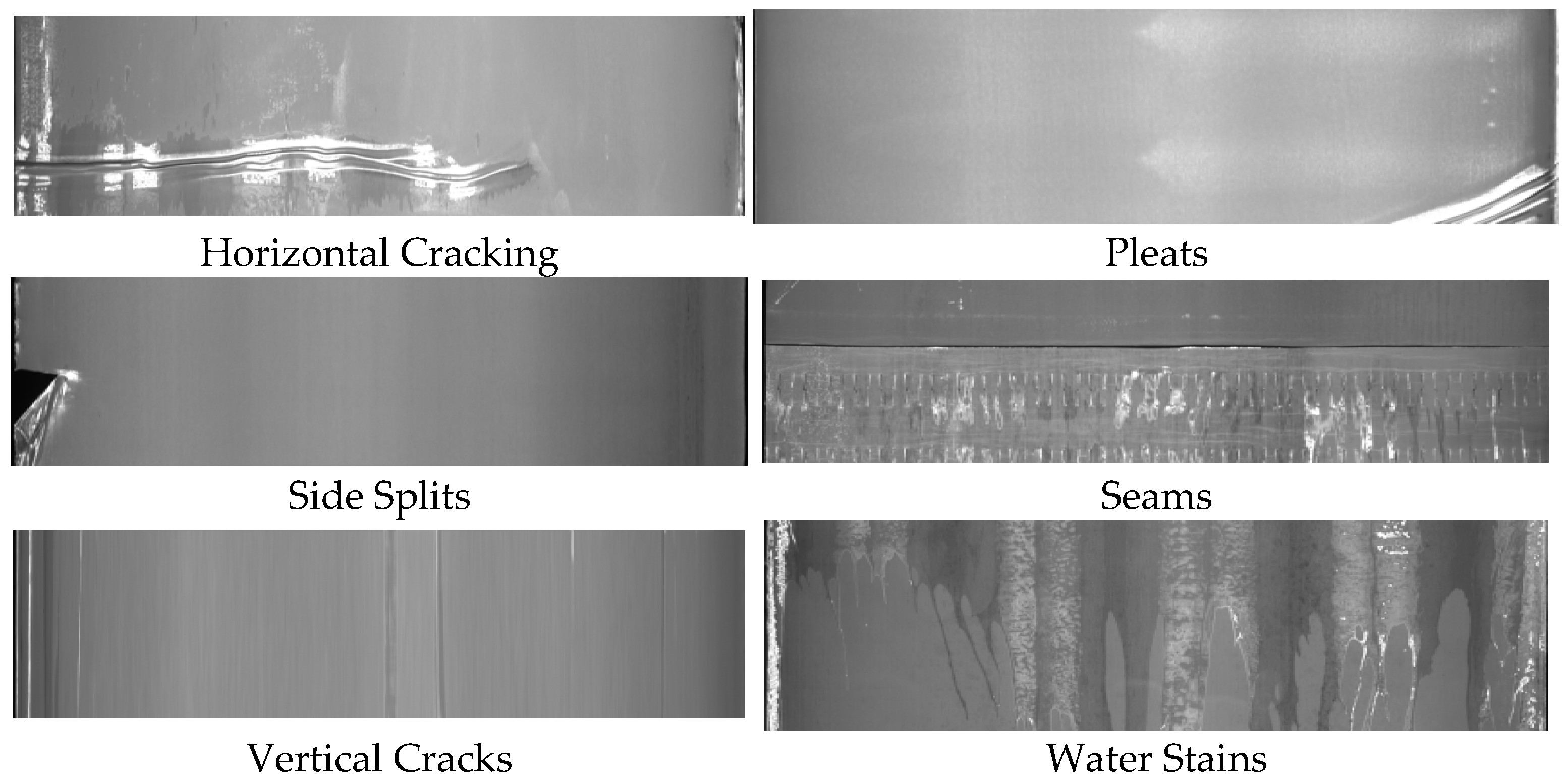
There are gaps in the images of hot-rolled strip steel surface defects acquired under different light intensities, light directions, etc. Therefore, the original images are normalized and pre-processed. In this paper, a sliding window of 128 × 128 pixels is used to intercept the whole CCD-captured hot-rolled strip surface defect images, and the complete defect as well as defect-free images are selected to establish a standard image dataset of hot-rolled strip surface defects, which reaches more than 60,000 standard sample images. This paper artificially augments the standard image dataset by adding rotated images to enhance model training quality, reaching a total of more than 120,000 standard sample images, which contain horizontal cracking, pleats, Side Splits, seams, vertical cracks, and water stains (as seen in Figure 3).

Among them, horizontal cracking has the greatest impact on the quality of hot-rolled strip and is the biggest safety hazard, while the effects of folds, pleats, side splits, seams, vertical cracks, and water stains decrease in order. The obtained standard sample image dataset was divided into 3 parts: partitioning the data into subsets based on a specific proportion (as shown in

Table 1. Standard defect image data set.

Dataset	Horizontal Cracking	Pleats	Vertical Cracks	Side Split	Seams	Water Stains	Total
Training set	20,000	20,000	15,000	15,000	15,000	15,000	100,000
Validation set	2000	2000	1500	1500	1500	1500	10,000
Test set	2000	2000	1500	1500	1500	1500	10,000

).

The dataset faces three main challenges: (1) defects within classes vary greatly in appearance; (2) defects between classes have similar aspects, and (3) the grayscale of defect images between classes can change due to the effect of defect images on illumination and material variations.

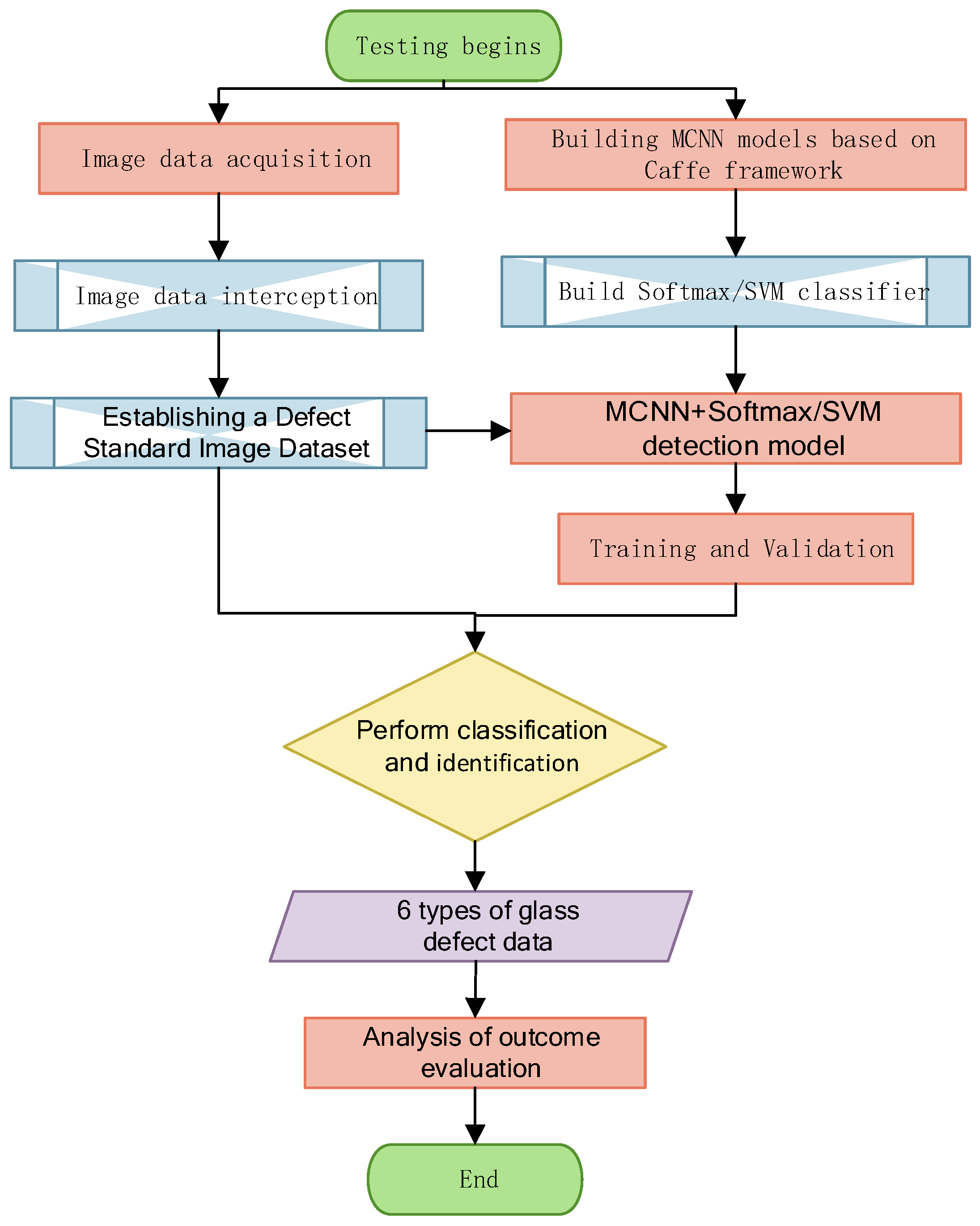
For the content and criteria of common defects on the surface of a hot-rolled strip of cover, this paper uses the constructed multi-scale convolutional neural network model to experimentally validate the detection of defects on the surface of a hot-rolled strip, and the main process is as follows:

Step 1. Selection of the Pytorch open-source framework for deep learning as the experimental environment for building multi-scale convolutional neural network models.

Step 2. While constructing the experimental environment, the CCD camera acquires image data of the surface of the hot rolled strip, and the images of the defects on the surface of the hot rolled strip obtained within the camera are processed and displayed on the monitor.

Step 3. Intercept the images of defects on the surface of the hot-rolled strip obtained in the camera, select the complete defective and defect-free images, normalize the detection of “defective images”, obtain the image size of 128 × 128, establish the defective standard image data set, and form the experimental sample.

Step 4. Training and validation of the samples based on a multiscale convolutional neural network model labeled with six types of defects.

Step 5. Randomly selected images from each category in the standard sample image dataset become the test samples, and the classification results and accuracy of the model to detect surface defects in images of hot-rolled strip steel are analyzed.

The whole process is shown in Figure 4.

4.2. Model Training

The MM models experimentally designed in this paper are performed based on the open-source framework of Pytorch deep learning, which provides a complete toolkit for training, testing, fine-tuning, and developing models. The models and corresponding optimizations are given in textual form rather than in code.

Steps during model training tests:

Step 1. Interception of the entire CCD-captured image of the hot-rolled strip surface defects using a sliding window of 128 × 128 pixels, selection of the complete defects, image normalization to obtain a standard defect picture, and collation into a standard defect data set.

Step 2. SIFT extraction of Gaussian differential pyramidal images from standard defect images to obtain a dataset for training a multi-scale convolutional neural network.

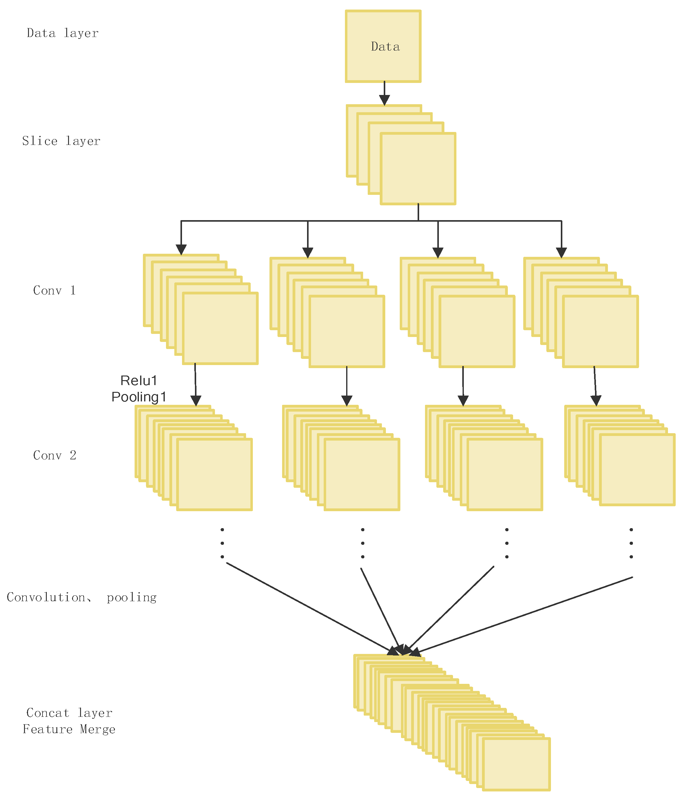
Step 3. The obtained multi-resolution image training data set is directly input to the network, and the four multi-scale images are divided by the slice layer and convolved separately to extract features. Initialize the network weights with “Gaussian”, where the bias is set to “Constant”.

Step 4. Select a batch training sample from the training set and input it into the network.

Step 5. Samples are propagated forward through the mapping between layers until Concat for feature merging, and then continue to propagate forward until the output layer to obtain the actual output vector.

Step 6. Calculates the error between the actual output vector and the label, and if the error is less than a predetermined threshold (or if the number of training iterations reaches a predetermined threshold), the network training is stopped; otherwise, the network continues.

Step 7. Tuning the weight parameters of the whole network model by backpropagation according to the principle of minimum error cost.

Step 8. Revert to Step 4 and continue the training.

Step 9. A randomly selected test dataset is fed into the trained model (convolutional kernel set, network weight parameters, etc.) for recognition detection.

The multi-scale defect image detection models constructed in this paper are all supervised training methods, and their training image sets are composed of vector pairs of (defect image, category label), where “defect image” is a normalized image, and the size of the image obtained after normalization is 128 × 128. The “category labels” represent the classification labels of the input defect images, which are divided into six categories: horizontal cracks, folds, vertical cracks, edge cracks, seams, and water stains.

In training, the experiments were conducted on the Ubuntu 20.04.2 LTS operating system, using the PyTorch deep learning framework and Python as the programming language. The CPU utilized was an Intel Core i7-9700F, while the GPU employed was an NVIDIA GeForce RTX 2080Ti. The images in the input layer are fixed-size 128 × 128 RGB images, and for the training set, the preprocessing is performed to subtract the average RGB value per pixel. The training network parameters are set as follows: The network uses the AdamW [34] optimization algorithm in the training phase to iteratively update the weights of the neural network based on the training data and the selected small batch training size; each batch contains 64 images. The weight decay is 0.005, the memory factor is 0.9, the learning rate is 0.001, and the learning strategy is STEP. The normalization factor is used to accelerate the training process in GPU mode, and the maximum number of training iterations is 1000.

4.3. Analysis of Results

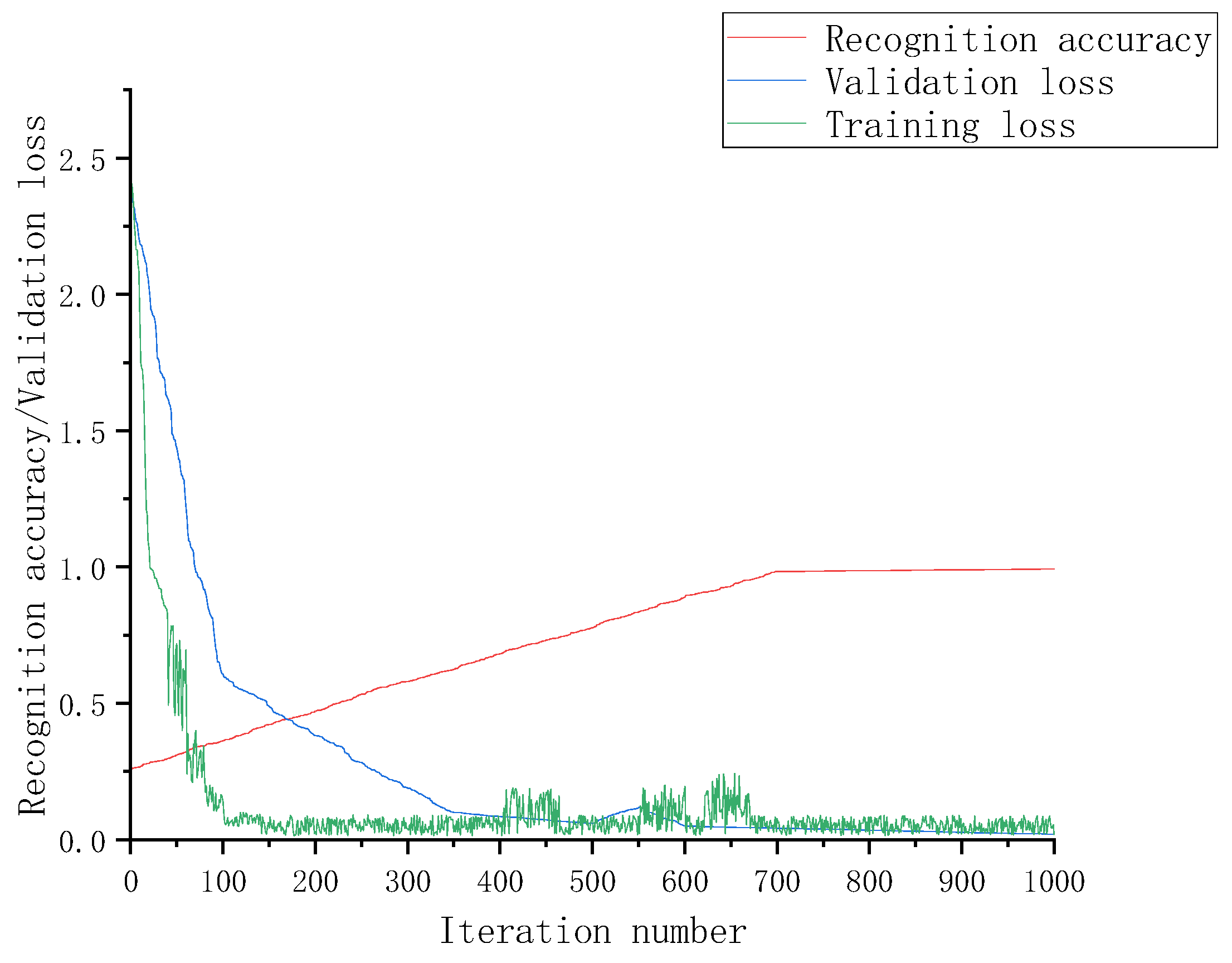
The Figure 5 illustrates the training process of the MM model network, including the curves for accuracy, training loss, and validation loss. It can be observed from the graph that with the increase in the number of iterations, the model’s accuracy on the validation set continues to rise while its loss decreases continuously. The model exhibits good convergence and achieves an accuracy of around 98.4% after 700 iterations.

To evaluate the performance of our classification model, we have introduced a confusion matrix, which serves as a valuable tool for assessing prediction accuracy. The confusion matrix is a square matrix that represents the relationship between actual and predicted classes. Rows of the matrix correspond to the true classes, while columns denote the predicted classes. Each element in the matrix represents the count of instances classified into a specific combination of true and predicted classes. As shown in

Table 2. Confusion matrices.

	Prediction of Horizontal Cracking	Prediction of Pleats	Prediction of Vertical Cracks	Prediction of Side Split	Prediction of Seams	Prediction of Water Stains
Actual Horizontal Cracking	1984	5	3	3	2	3
Actual Pleats	10	1987	1	1	0	1
Actual Vertical Cracks	6	5	1486	2	1	0
Actual Side Splits	4	4	1	1488	1	2
Actual Seams	5	2	1	2	1490	0
Actual Water Stains	2	0	0	1	3	1494

.

The first row represents the samples with the true label “horizontal cracking”. Among these samples, 1984 were correctly predicted as “horizontal cracking”, 5 were wrongly predicted as “pleats”, 3 were wrongly predicted as “vertical cracks “, 3 were wrongly predicted as “side splits”, 2 were wrongly predicted as “seams”, and 3 were wrongly predicted as “water stains”.

The second row represents the samples with the true label “pleats”. Among these samples, 10 were wrongly predicted as “horizontal cracking”, 1987 were correctly predicted as “pleats”, 1 was wrongly predicted as “vertical cracks”, 1 was wrongly predicted as “side splits”, 0 were wrongly predicted as “seams”, and 1 was wrongly predicted as “water stains”.

The following rows follow the same pattern, representing the remaining labels. This confusion matrix helps us understand the performance of the MM model for each defect type and the possible misclassification of the model situation.

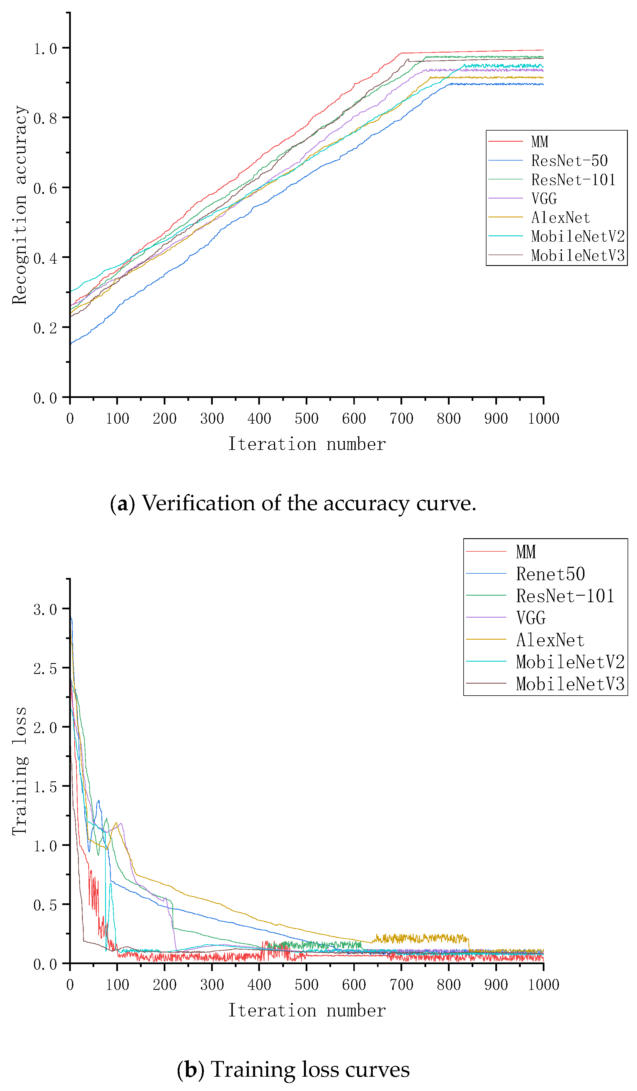
To verify the impact of different modules on network performance, five evaluation indices were introduced in this article: computing power, which refers to the number of floating-point operations executed per second (FLOPs), feature memory, recall, F1 score, and accuracy. The MM network was compared with four popular classical networks (ResNet-101, ResNet-50, VGG, and AlexNet) as well as the new lightweight neural networks MobileNetV2 and MobileNetV3.

Table 3. Comparison of the comprehensive performance of different networks.

Models	Precision	Feature Memory	Number of Floating-Point Operations (FLOPs)	Recall	F1
Resnet-50	89.7%	60 MB	10 GFLOPs	87.2%	0.92
ResNet-101	97.38%	155 MB	8 GFLOPs	92.6%	0.93
VGG	93.56%	96 MB	15.5 GFLOPs	93.7%	0.90
AlexNet	91.30%	300 MB	0.72 GFLOPs	91.6%	0.92
MobileNetV2	94.6%	57 MB	0.98 GFLOPs	94.6%	0.95
MobileNetV3	96.7%	52 MB	0.76 GFLOPs	95.4%	0.97
MM	98.06%	50 MB	0.67 GFLOPs	98.7%	0.99

shows the detailed comparison results.

After 1000 iterations, AlexNet, ResNet-50, and VGG achieved classification accuracies of 91.30%, 89.7%, and 93.56%, respectively, while ResNet-101, MobileNetV2, and MobileNetV3 achieved slightly better accuracies of 97.38%, 94.6%, and 96.7%, respectively. Compared to Resnet50, MM increased the accuracy by 8.36 percentage points, by 0.38 percentage points compared to ResNet-101, by 4.5 percentage points compared to VGG, by 6.76 percentage points compared to AlexNet, by 3.46 percentage points compared to MobileNetV2, and by 1.36 percentage points compared to MobileNetV3. Additionally, MM had a faster decrease in training loss compared to the other models, with a final loss value approaching zero as shown in Figure 6. Moreover, MM had smaller feature memory and fewer floating-point computations, while its recall and F1 metrics were relatively higher. These results fully demonstrate that the key-point feature convolutional operation reduces the number of network parameters and that the key-point feature set mapping fusion operation promotes information exchange between key points, making it effective in reducing performance losses.

From the comprehensive analysis of the experiments above, MM has the best performance in all indicators. Resnet-50, ResNet-101, VGG, AlexNet, MobileNetV2, and MobileNetV3 models lack the ability to detect small defects on the surface of steel. The MM proposed in this paper, with the fusion encoding module as the core, constructs a multiscale neural network model through the Gaussian difference pyramid. It not only improves the network’s capture ability for different resolution modes but also achieves better model accuracy and efficiency. The recognition accuracy on the steel surface defect dataset is the best. The recognition accuracy of various neural network models for different types of defects is shown in

Table 4. Accuracy of different networks for defect recognition in various categories.

Transverse Crack	ResNet-50	ResNet-101	VGG	AlexNet	MobileNetV2	MobileNetV3	MM
Horizontal Cracking	92.4%	91.6%	86.2%	92.1%	91.2%	92.6%	99.2%
Pleats	72.6%	98.2%	82.9%	97.2%	97.7%	97.2%	99.3%
Side Splits	93.2%	97.2%	92.6%	92.2%	98.6%	98.6%	99.2%
Seams	81.7%	98.9%	93.5%	93.2%	95.8%	93.5%	99.3%
Water Stains	91.2%	99.7%	92.4%	95.2%	96.6%	99.2%	99.6%
Vertical cracks	93.9%	93.2%	97.9%	96.2%	94.2%	98.7%	99.0%

.

5. Conclusions

To address the issues of increasing parameter count and computational cost in convolutional neural networks as well as the challenge of preserving key-point feature information in existing lightweight networks, this paper proposes a novel lightweight network, referred to as MM. The core of this model is a fusion encoding module that leverages Gaussian difference pyramids to construct a multi-scale neural network model. By enhancing the network’s ability to capture patterns at different resolutions, the proposed model achieves higher model accuracy and efficiency. Experimental results show that the network avoids the loss of feature information at key points, improves the classification accuracy, and significantly improves the overall performance compared with other networks, which provides strong support for the mobile classification task of steel surface defects. It provides strong support for the mobile deployment of steel surface defect classification tasks. In the future, we plan to improve the model’s ability to perform well on new data and optimize it to meet the requirements for commercialization. Furthermore, the proposed model can be applied to real-time object detection and tracking tasks, mobile device applications, and image super-resolution reconstruction. These directions leverage the lightweight nature and multi-scale capabilities of MM, offering possibilities for real-time image analysis, edge computing, and enhanced image processing in various domains.