A Distribution-Preserving Under-Sampling Method for Imbalance Defect Recognition in Castings

Abstract

Data imbalance is a crucial factor that limits the performance of automatic defect recognition systems in castings. The bias and deterioration of the model are generated by massive normal samples and minor defect samples. Traditional re-sampling methods randomly change the data distribution and ignore the significant intra-class difference among all normal samples. Therefore, this paper proposes a distribution-preserving under-sampling method for imbalance defect-recognition in castings. In detail, our method divides all normal samples into several sub-groups by cluster analysis and reassembles them into some balance datasets, which makes the normal samples in all balance datasets have an identical distribution with the original imbalance dataset. Finally, experiments on our dataset with 3260 images indicate that the proposed method achieves a 0.816 AUC (area under curve) score, which demonstrates significant advantages compared to cost-sensitive learning and re-sampling methods.

1. Introduction

Casting is an important forming means to achieve high-efficiency and low-cost manufacture and is an irreplaceable process for metal parts with complex structure. A large number of core components are formed by the casting process in the high-end manufacturing industry. Unfortunately, castings inevitably have different internal defects because of casting materials and processes. These internal defects will seriously affect the mechanical properties of castings, even directly leading to scrap.

To obtain the internal information of castings, digital radiography (DR) technology is utilized and gradually became the first choice for nondestructive testing. DR utilizes X-ray to penetrate the castings and directly produces a digital image through the digital detector array (DDA). Then, the inspectors judge whether there is a defect in the casting by observing the change of gray level in the digital image. However, manual visual inspection not only is laborious and inefficient but also easy to be affected by the ability and experience of the inspectors. Consequently, automatic defect recognition (ADR) has collected much attention and became one of the research hot points. Early research about ADR mainly focused on handcrafted feature extraction and traditional machine learning. Mery et al. [1] utilized a single filter to track potential defects in image sequences. Hernandez et al. [2] used the neuro-fuzzy method to classify the defect and normal samples. Zhao et al. [3] proposed a defect recognition framework for automobile wheels, which employed the gray arranging pairs method to segment the defects, then their randomly distributed triangle features were extracted and fed into a sparse representation classifier to achieve defect classification. Overall, these approaches heavily rely on the handcrafted features designed by experts. Unfortunately, the handcrafted features usually have poor robustness, which fails to adapt to the change of position, structure, and ray intensity.

As deep learning develops, current ADR systems in casting mainly realize defect recognition through a convolutional neural network (CNN). Du et al. [4] used the Faster-RCNN [5] with feature pyramid networks (FPN) [6] to locate the defect. Yu et al. [7] proposed an adaptive CNN model to realize multi-class defect segmentation. A variable attention nested UNet++ network [8] was introduced for defect segmentation in the X-ray image.

The above research aims to achieve end-to-end defect location and segmentation, which can provide more comprehensive information about the defect. However, they also have a slow detection speed. In actual detection, the number of images without defects is far more than the number of images with defects. Thus, the image-level recognition method can be deployed at the front of the entire detection process to improve detection efficiency. Mery et al. [9] extensively tested the combined performance of multiple features and classifiers in the GDX-ray [10] dataset. This work crops the original image into enormous, small patches (32 × 32). Because of low resolution, deep learning methods perform worse than traditional machine learning. Subsequently, Mery [11] used GAN and physical simulation methods to produce more virtual defect images and boost accuracy. Tang et al. [12] combined spatial attention mechanisms and bi-linear pooling into a CNN model to increase the representation power. Similar to [12], Hu et al. [13] presented a two-stage training procedure, which firstly forces the network to classify the casting type and then to classify the defect and normal samples. Jiang et al. [14] presented the mutual-channel loss and an attention-guided data augmentation method to boost the original VGG network.

Regrettably, the above research is dedicated to designing higher performance CNN on balance datasets and sidestepping the fact of class imbalance that significantly impacts the recognition accuracy. At present, there are two main solutions to solve the imbalance classification: the re-weighting and the re-sampling method. The re-weighting method is also called cost-sensitive learning. It adopts re-weighting strategies to adjust the loss of minor class samples. Weighted cross-entropy loss is the simplest way whose weight is the inverse class frequencies. Seesaw loss [15] adaptively re-balances gradients of minor-class and major-class samples with mitigation factor and the compensation factor. Focal loss [16] is proposed to solve the class imbalance in object detection. It inversely re-weights classes by prediction probabilities, so that it can give higher weights to the minor classes but lower weights to the major classes. The re-sampling method [17,18] directly changes the data distribution and forms some balance datasets by randomly over-sampling the minority class or under-sampling the majority class.

However, the random re-sampling method ignores the intra-class difference in defect recognition. As shown in Figure 1, these normal samples are different in gray level, texture, and so on. In Figure 1a, this kind of image is brighter than others. In Figure 1b, such images have some false defects because of the concave-convex surface of castings. Figure 1c stands for the rest of the samples whose background lacks detail. Based on the previous analysis, the random under-sampling method will change the original distribution information in all normal samples and lead to the variability of balance datasets generated by re-sampling. It will break the important assumption in deep learning: independent identical distribution. Considering this, a distribution-preserving under-sampling method is proposed for imbalance defect recognition in castings. By cluster analysis, we divide all normal samples into several groups and reassemble them into some balance datasets. The normal samples in these balance datasets follow a similar distribution to the original data. Benefitting from the above improvement, our methods achieve a better accuracy under imbalanced data.

2. Methods

2.1. Overview

In this section, we present our method for imbalance defect recognition. Our method firstly extracts the image features of normal samples by a pre-trained network, and then clusters them into some groups based on k-means++ [19] approach. Some normal samples belonging to each group are selected and recombined to form several new subsets. Each new subset is combined with all defect samples, resulting in some balance training datasets. We train our deep learning model by each training dataset and obtain some network weights. Through model fusion, our method produces better performance under an imbalanced dataset. The details are shown in Figure 2.

2.2. Distribution-Preserving Under-Sample

Assume that a class-imbalanced dataset D = {D_n ∪ D_d} includes normal samples (D_n) and defect samples (D_d). The numbers of the D_n, D_d are N_n, N_d. N_n is far larger than N_d. Our goal is to build some balanced datasets through under-sample methods for relieving the imbalance.

Traditional under-sample methods select some samples randomly. However, this method will change the prior distribution information in the normal class because of large intra-class differences. We believe that the subsets obtained after under-sampling should maintain the same distribution as the original dataset. Motivated by this, a distribution-preserving under-sample method is proposed to acquire multiple subsets that are identically distributed with the original normal class.

For our method, a ResNet18 [20] pre-trained by ImageNet [21] is first employed to extract the high-dimension features of normal samples because it has been proven to be a good feature extractor. These features are then PCA-reduced to 128 dimensions, whitened, and L2-normalized. K-means++, a standard clustering approach, is widely used and can be regarded as a baseline clustering method. It takes the reduced dimension features as input and clusters them into K distinct groups (G₁, G₂, …, G_k) based on an Euclidean distance. Each group represents the sub-class of the normal sample.

To ensure the same distribution between each subset and the original dataset, we randomly select p% of the samples from each group and repeat t times, so several sub-groups (G₁₁, G₁₂, …, G_1t, …, G_kt) are formed. Finally, t balanced datasets (BD₁, BD₂, …, BD_t) are aggregated by:

BD_i = {G_1i ∪ G_2i ∪, …, G_ki ∪ D_d}, i = 1, 2, …, t,

(1)

The number of normal samples in each BD can be computed as follows:

N_BD = N_n × p%,

(2)

In general, CNN does not need a totally balanced dataset, so we set the N_BD slightly larger than N_d by adjusting p.

2.3. Network

CNN has demonstrated impressive ability in many computer vision tasks. It can automatically extract general and robust features from the input data by back-propagation. CNN is usually composed of convolution, activation functions, and fully connected layers. Through careful designing of network architecture, a multiple classical CNN model is proposed. In this work, we consider the network performance and inference time comprehensively; ResNet18 and MobileNetV2 [22] are selected for defect recognition.

ResNet is used to solve the gradient disappearance with the increase in network depth. The main idea of ResNet is to introduce a residual block that forces the network to learn identity mapping rather than fitting ground truth directly. Through stacking some residual blocks, multiple versions of ResNet are produced, such as ResNet18, ResNet50 ResNet101, and so on. MobileNetV2 is improved based on ResNet to make it lighter, which proposed the inverted residual block. Different from the residual block, this module first expands the channel of input features to a high dimension and filters it with a lightweight depth-wise convolutional layer. The features are subsequently projected back to a low dimension with a 1 × 1 convolution. The details of the residual block and inverted residual block are shown in Figure 3.

In this study, ResNet18 and MobileNetV2 are modified to adapt to this task. We employ the pre-trained weight from ImageNet as an initialization and remove their all fully connected layers. Then, a new fully connected layer is added to the network. The softmax layer transfers the output of the fully connected layer into a probability distribution. Finally, we train t CNN models based on t balanced datasets.

2.4. Model Fusion

Although our under-sample method can produce several balanced and identically distributed datasets, it just includes part of the whole normal samples. The model trained by different datasets must have some bias which is harmful to generalization performance. Thus, we employ the model fusion strategy to solve it. Suppose $f_i$ is the CNN model trained by BD_i, ${\theta }_i$ is the parameter of it. $f_i(x,{\theta }_i)$ stands for the CNN output of the sample $x$. By averaging the output of multiple CNN, the result $y$ without bias can be obtained.

$$y={\displaystyle \sum _{i=1}^t{f}_i}(x,{\theta }_i)$$

(3)

3. Experimental Setup

3.1. Datasets

We collect 3260 X-rays whose resolution is 480 × 480 of aluminum alloy castings from the line for evaluating our method. There are 630 defective samples and 2630 normal samples in the total dataset. The training dataset is imbalanced to keep consistent with the actual task for defect recognition. The evaluation and test datasets are balanced for a better comparison.

Table 1. The number of samples in this dataset.

Dataset	Normal	Defect	Total
Train	2430	430	2860
Validation	100	100	200
Test	100	100	200

shows the detailed number. Figure 4 shows some typical normal and defect samples.

3.2. Implementation Details

The computation platform used in this work was Intel Core i9-9920X, 64G memory, and TITAN-RTX with 24G GPU memory. All the models were implemented by the MindSpore frame framework. The optimizer is Adam. The batch size and the learning rate were 16 and 0.001, respectively.

3.3. Evaluation Metric

Accuracy is usually used for evaluating the balance classification task. However, the tolerance for normal samples to be detected as defective samples is far greater than that for defective samples to be detected as normal samples. So, accuracy is not entirely suitable for evaluating it. In this task, AUC (area under curve) score is the main evaluation metric. AUC score is obtained by calculating the area under the ROC (receiver operating characteristic) with multi-thresholds. When the threshold is 0.5, precision and recall are also reported. The specific calculation formula of precision and recall are as follows:

$$\mathit{Presicion}=\frac{TP}{TP+FP}$$

(4)

$$Recall=\frac{TP}{TP+FN}$$

(5)

TP and FN are the numbers of defect samples classified correctly or not. FP represents the number of normal samples classified incorrectly.

4. Results and Discussion

4.1. Compare with Other Methods

In order to illustrate the advancement of our method, we compare it to other methods of imbalance classification including cost-sensitive learning and re-sampling method. At the same time, we test our method under two different backbone networks to prove its generalization. Every method is tested five times and the results are shown in

Table 2. The quantification results of different methods towards class-imbalance classification.

Backbone	Method	Precision	Recall	AUC
ResNet18	CE loss	0.5005 ± 0.001	0.996 ± 0.008	0.5509 ± 0.0735
	WCE loss	0.668 ± 0.0333	0.846 ± 0.0301	0.7437 ± 0.0291
	Focal loss	0.538 ± 0.0571	0.494 ± 0.2463	0.5613 ± 0.0435
	Seesaw loss	0.668 ± 0.0098	0.89 ± 0.0482	0.74 ± 0.0232
	Over-sample	0.6534 ± 0.0163	0.824 ± 0.0508	0.7797 ± 0.0202
	Under-sample	0.6537 ± 0.0757	0.75 ± 0.1838	0.7408 ± 0.035
	Ours	0.6326 ± 0.0227	0.84 ± 0.0562	0.7891 ± 0.0168
MobileNetV2	CE loss	0.5 ± 0.0	1 ± 0	0.5101 ± 0.075
	WCE loss	0.709 ± 0.0256	0.846 ± 0.0287	0.7864 ± 0.0355
	Focal loss	0.529 ± 0.0208	0.598 ± 0.0838	0.5408 ± 0.0194
	Seesaw loss	0.675 ± 0.037	0.868 ± 0.0343	0.7656 ± 0.0236
	Over-sample	0.6712 ± 0.0316	0.84 ± 0.0701	0.7786 ± 0.0153
	Under-sample	0.6674 ± 0.0203	0.8224 ± 0.0528	0.7859 ± 0.0069
	Ours	0.6398 ± 0.0155	0.9080 ± 0.0192	0.8158 ± 0.0160

. The baseline is the CNN model trained with standard cross-entropy loss. The baseline considers all samples as normal samples and produces the worst result due to extreme imbalance. Cost-sensitive learning improves it by giving less weight to normal samples. Simple weight cross-entropy loss performs better than focal and seesaw loss. Re-sampling methods also achieve higher accuracy. When ResNet18 is used as the backbone network, the over-sample method performs better than the under-sample, but when the backbone network is MobileNetV2, under-sample performs better than the over-sample method. In general, re-sampling methods are more suitable for our dataset than cost-sensitive learning. Our method achieves the best result under different backbone networks, especially MobileNetV2. The AUC score of our method is 3.8% higher than the under-sample method, which proves the effectiveness of our approach.

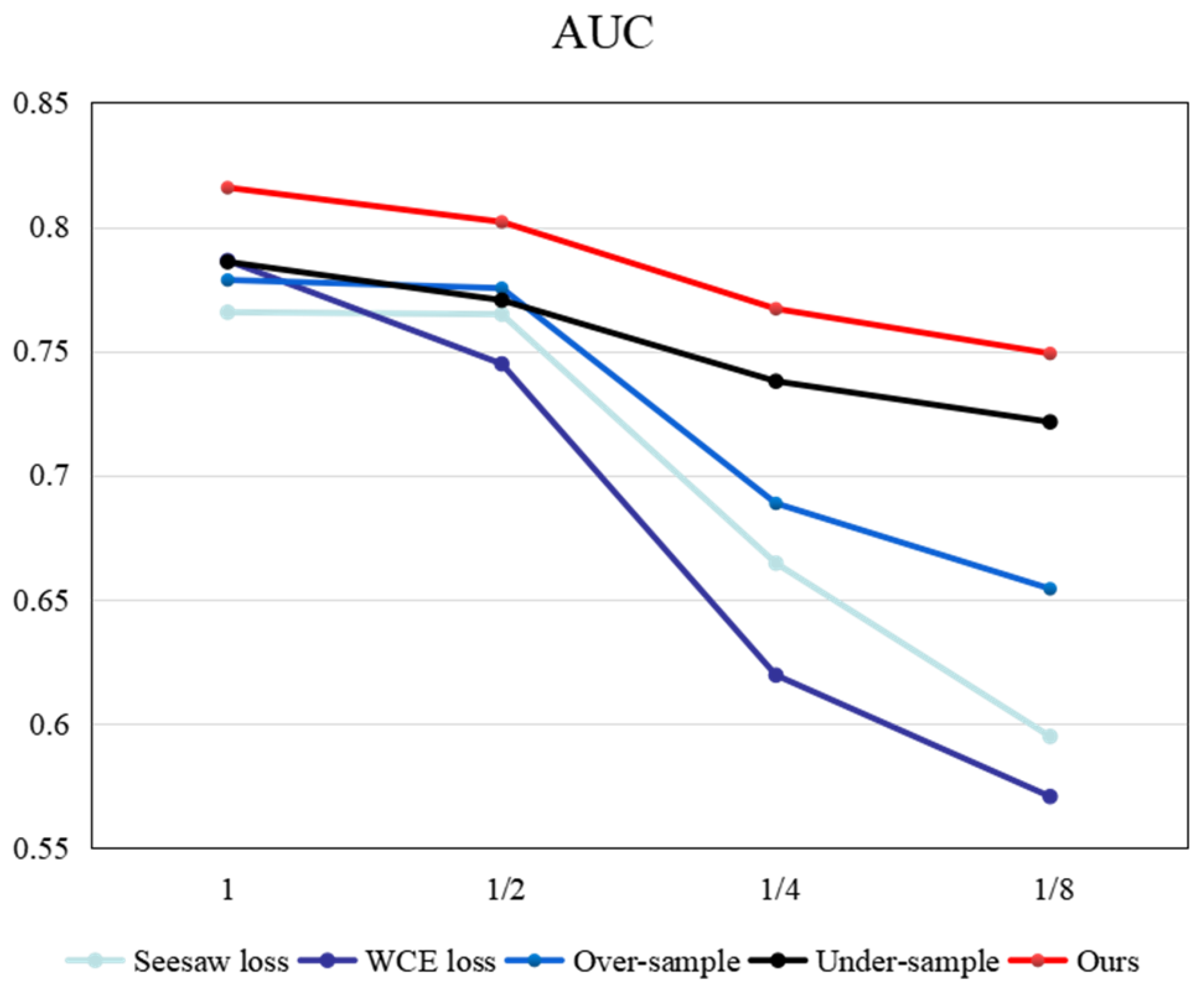
4.2. The Influence on Different Imbalance Ratios

To prove the robustness of our method, a further experiment is conducted under different imbalance ratios (normal sample/defect sample). We gradually reduce part of the defect samples in the training dataset for simulating the more imbalanced situation. MobileNetV2 is utilized as the backbone network and part of the cost-sensitive learning methods and re-sampling methods are employed to make a comparison with our approach based on the results in 4.1. We also adjust the weight factors according to the imbalance ratios for WCE and seesaw loss methods. Figure 5 shows the AUC scores of different methods when the number of defect samples reduces to 1/2, 1/4, 1/8, and 1/16 of the original. It is consistent with the intuition that the experimental performance of most comparison methods significantly decreases as the number of defect samples decreases. Overall, the tolerance of cost-sensitive learning methods is worst for imbalanced datasets. When the defect samples are only 1/8 of the original, the AUC of seesaw loss reduces by 27.45%. This is because these methods cannot essentially deal with the issue of lacking information, particularly on limited data amounts. Re-sampling methods perform better than cost-sensitive learning methods, especially the under-sampling method. However, it still has a big gap with our method. As the number of defect samples decreases, the AUC score of our method is still optimal. It demonstrates that our method has significant advantages in tolerance for imbalance.

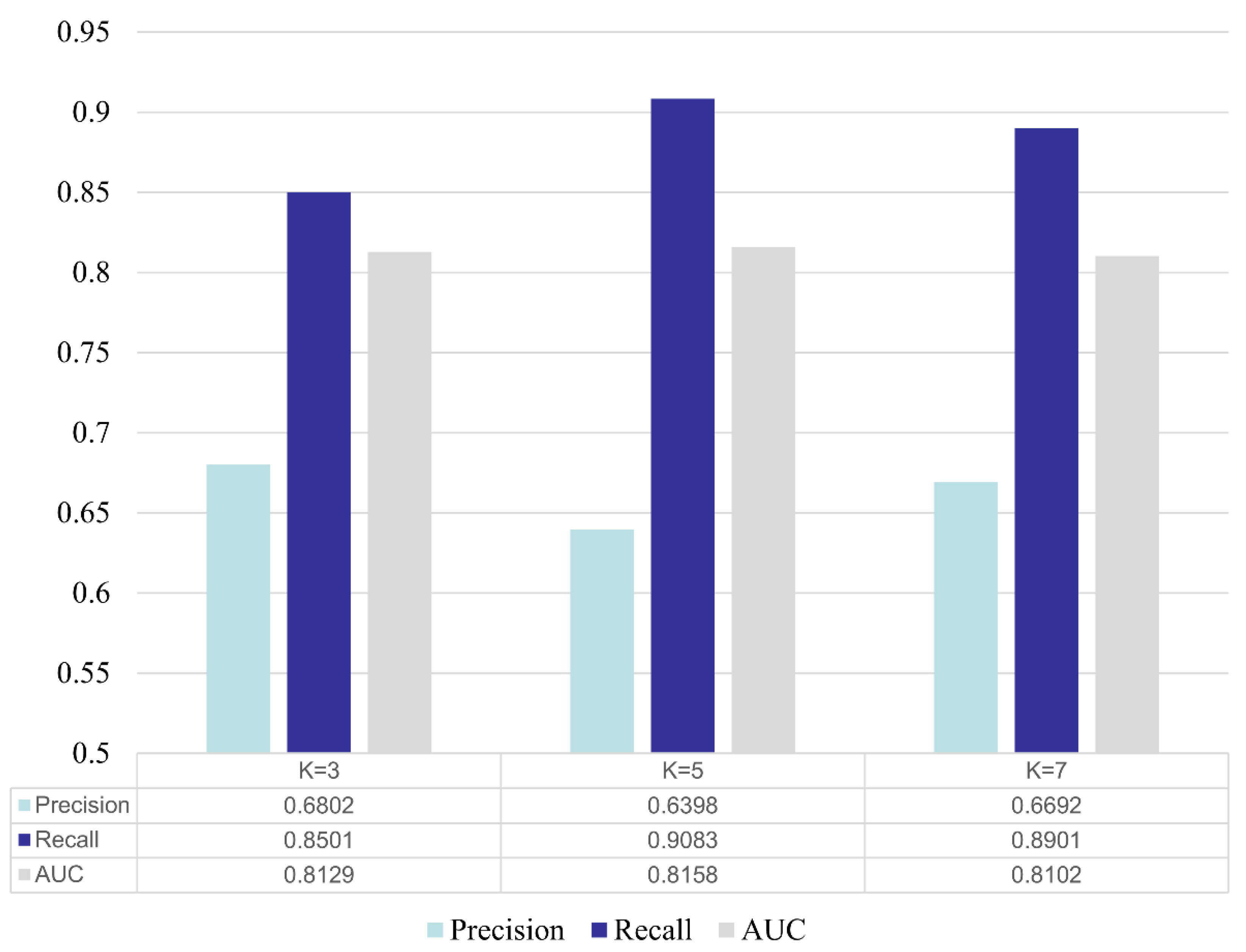
4.3. The Influence on Cluster Number K

Cluster number K is an important parameter for the k-means++ algorithm. Different K will lead to a different cluster result. We set a series of K (3, 5, 7) and observe the impact on the result in Figure 6. Experiments show that our method is not sensitive to the choice of cluster number K. Different K can achieve similar performance. Although the number of clusters is different, our method has the same sampling proportion in different sub-groups, which ensures the distribution consistency between each balanced dataset and the original dataset. This mechanism makes our method more robust on hyper-parameter, that is, the cost of applying this method is low.

5. Conclusions

Data imbalance is very common in casting defect recognition. This paper proposes a distribution-preserving under-sampling method for reducing the uncertainty of traditional re-sampling methods. Our method divides all normal samples into several sub-groups by k-means++ and reassembles them into some balance datasets, which makes the normal samples in all balance datasets have an identical distribution with the original imbalance dataset. Experiments on our dataset illustrate that the proposed method achieves significant advantages compared to the state-of-the-art methods for data imbalance. At the same time, our method is more resistant to extreme data imbalance and not sensitive to the hyper-parameter.

References

1. Mery, D.; Filbert, D. Automated flaw detection in aluminum castings based on the tracking of potential defects in a radioscopic image sequence. IEEE Trans. Robot. Autom. 2002, 18, 890–901. [Google Scholar] [CrossRef] [Green Version]
2. Hernández, S.; Sáez, D.; Mery, D.; Silva, R.D.; Sequeira, M. Automated defect detection in aluminum castings and welds using neuro-fuzzy classifiers. In Proceedings of the 16th World Conference on NDT, Montreal, QC, Canada, 30 August 2004. [Google Scholar]
3. Zhao, X.; He, Z.; Zhang, S.; Liang, D. A sparse-representation-based robust inspection system for hidden defects classification in casting components. Neurocomputing 2015, 153, 1–10. [Google Scholar] [CrossRef]
4. Du, W.; Shen, H.; Fu, J.; Zhang, G.; He, Q. Approaches for improvement of the X-ray image defect detection of automobile casting aluminum parts based on deep learning. NDT E Int. 2019, 107, 102144. [Google Scholar] [CrossRef]
5. Ren, S.; He, K.; Girshick, R.; Sun, J. Faster R-CNN: Towards Real-Time Object Detection with Region Proposal Networks. IEEE Trans. Pattern Anal. Mach. Intell. 2015, 39, 1137–1149. [Google Scholar] [CrossRef] [PubMed] [Green Version]
6. Lin, T.Y.; Dollár, P.; Girshick, R.; He, K.; Hariharan, B.; Belongie, S. Feature Pyramid Networks for Object Detection. In Proceedings of the IEEE Conference on Computer Vision and Pattern Recognition, Honolulu, HI, USA, 21 July 2017. [Google Scholar]
7. Yu, H.; Li, X.; Song, K.; Shang, E.; Liu, H.; Yan, Y. Adaptive depth and receptive field selection network for defect semantic segmentation on castings X-rays. NDT E Int. 2020, 116, 102345. [Google Scholar] [CrossRef]
8. Liu, J.; Kim, J.H. A Variable Attention Nested UNet++ Network-Based NDT X-ray Image Defect Segmentation Method. Coatings 2022, 12, 634. [Google Scholar] [CrossRef]
9. Mery, D.; Arteta, C. Automatic Defect Recognition in X-Ray Testing Using Computer Vision. In Proceedings of the IEEE Winter Conference on Applications of Computer Vision, Santa Rosa, CA, USA, 27 March 2017. [Google Scholar]
10. Mery, D.; Riffo, V.; Zscherpel, U. GDXray: The Database of X-ray Images for Nondestructive Testing. J. Nondestruct. Eval. 2015, 34, 1–12. [Google Scholar] [CrossRef]
11. Mery, D. Aluminum Casting Inspection Using Deep Learning: A Method Based on Convolutional Neural Networks. J. Nondestruct. Eval. 2020, 39, 1–12. [Google Scholar] [CrossRef]
12. Tang, Z.; Tian, E.; Wang, Y.; Wang, L.; Yang, T. Non-destructive defect detection in castings by using spatial attention bilinear convolutional neural network. IEEE Trans. Ind. Inform. 2020, 17, 82–89. [Google Scholar] [CrossRef]
13. Hu, C.; Wang, Y. An efficient cnn model based on object-level attention mechanism for casting defects detection on radiography images. IEEE Trans. Ind. Electron. 2020, 67, 10922–10930. [Google Scholar] [CrossRef]
14. Jiang, L.; Wang, Y.; Tang, Z.; Miao, Y.; Chen, S. Casting defect detection in X-ray images using convolutional neural networks and attention-guided data augmentation. Measurement 2021, 170, 108736. [Google Scholar] [CrossRef]
15. Wang, J.; Zhang, W.; Zang, Y.; Cao, Y.; Pang, J.; Gong, T.; Chen, K.; Liu, Z.; Loy, C.C.; Lin, D. Seesaw loss for long-tailed instance segmentation. In Proceedings of the IEEE/CVF Conference on Computer Vision and Pattern Recognition, Nashville, TN, USA, 19 June 2021. [Google Scholar]
16. Lin, T.Y.; Goyal, P.; Girshick, R.; He, K.; Dollár, P. Focal loss for dense object detection. In Proceedings of the IEEE International Conference on Computer Vision, Venice, Italy, 22 October 2017. [Google Scholar]
17. Estabrooks, A.; Jo, T.; Japkowicz, N. A multiple resampling method for learning from imbalanced data sets. Comput. Intell. 2004, 20, 8–36. [Google Scholar] [CrossRef]
18. Liu, X.-Y.; Wu, J.; Zhou, Z.-H. Exploratory undersampling for class-imbalance learning. IEEE Trans. Syst. Man Cybern. 2008, 39, 539–550. [Google Scholar]
19. Arthur, D.; Vassilvitskii, S. K-means++: The Advantages of Careful Seeding. In Proceedings of the Eighteenth Annual ACM-SIAM Symposium on Discrete Algorithms, Miami, FL, USA, 22 January 2006. [Google Scholar]
20. He, K.; Zhang, K.; Ren, S.; Sun, J. Deep residual learning for image recognition. In Proceedings of the IEEE Computer Society Conference on Computer Vision and Pattern Recognition, Las Vegas, NV, USA, 16 June 2016. [Google Scholar]
21. Deng, J.; Dong, W.; Socher, R.; Li, L.J.; Li, K.; Fei-Fei, L. ImageNet: A Large-Scale Hierarchical Image Database. In Proceedings of the IEEE Computer Society Conference on Computer Vision and Pattern Recognition, Miami, FL, USA, 18 June 2009. [Google Scholar]
22. Sandler, M.; Howard, A.; Zhu, M.; Zhmoginov, A.; Chen, L.C. MobileNetV2: Inverted Residuals and Linear Bottlenecks. In Proceedings of the IEEE/CVF Conference on Computer Vision and Pattern Recognition, Salt Lake City, UT, USA, 17 June 2018. [Google Scholar]
Figure 1. Three typical normal samples. (a): brighter normal samples (b): normal samples with false defects (c): normal samples with missing details.
Coatings 12 01808 g001
Figure 2. The pipeline of the proposed method.
Coatings 12 01808 g002
Figure 3. (a): residual block (b): inverted residual block, n means channel numbers.
Coatings 12 01808 g003
Figure 4. (a): normal samples (b): defect samples.
Coatings 12 01808 g004
Figure 5. The AUC scores under different imbalance ratios.
Coatings 12 01808 g005
Figure 6. The results of the proposed method under different cluster number.
Coatings 12 01808 g006