TSSTNet: A Two-Stream Swin Transformer Network for Salient Object Detection of No-Service Rail Surface Defects

Abstract

The detection of no-service rail surface defects is important in the rail manufacturing process. Detection of defects can prevent significant financial losses. However, the texture and form of the defects are often very similar to the background, which makes them difficult for the human eye to distinguish. How to accurately identify rail surface defects thus poses a challenge. We introduce salient object detection through machine vision to deal with this challenge. Salient object detection locates the most “significant” areas of an image using algorithms, which constitute an integral part of machine vision inspection. However, existing saliency detection networks suffer from inaccurate positioning, poor contouring, and incomplete detection. Therefore, we propose an innovative deep learning network named Two-Stream Swin Transformer Network (TSSTNet) for salient detection of no-service rail surface defects. Specifically, we propose a two-stream encoder—one stream for feature extraction and the other for edge extraction. TSSTNet also includes a three-stream decoder, consisting of a saliency stream, edge stream, and fusion stream. For the problem of incomplete detection, we innovatively introduce the Swin Transformer to model global information. For the problem of unclear contours, we expect to deepen the understanding of the difference in depth between the foreground and background through the learning of contour maps, so the contour alignment module (CAM) is created to deal with this problem. Moreover, to make the most of multimodal information, we suggest a multi-feature fusion module (MFFM). Finally, we conducted comparative experiments with 10 state-of-the-art (SOTA) approaches on the NRSD-MN datasets, and our model performed more competitively than others on five metrics.

1. Introduction

Rail quality inspection is very important in the rail production process in steel mills, and one of the most critical aspects is the detection of rail surface defects. Earlier detection of no-service rail surface defects can prevent economic losses and safety accidents from occurring in time.

The rails to be inspected are divided into the in-service and no-service rails, which usually have different defect maps. Images of in-service rail defects often have bright backgrounds, prominent weaknesses, and distinct contours. However, no-service rail defect maps often have dark backgrounds, uneven lighting, and impurities of various origins interfering with identification, which can easily cause different shapes of rail surface defects during the processing:

(1)

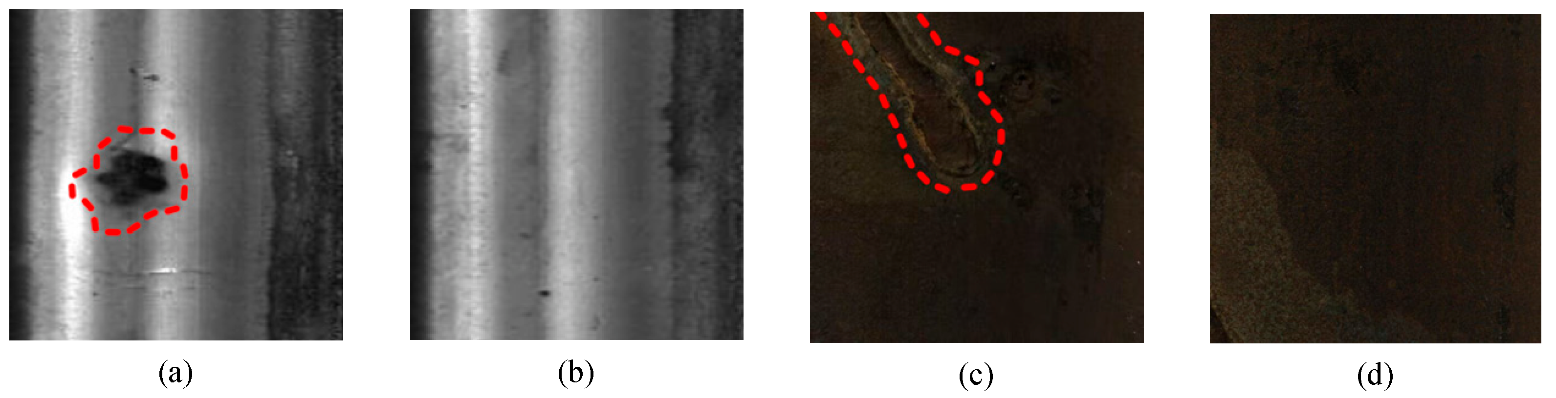
When the rail is heated, due to unreasonable technology and techniques, thermal stresses are created in the rail material, forming cracks on the surface;

(2)

If the billet is not cleaned or is cleaned improperly, the impurities attached to the billet remain on the surface of the finished rail after heating and rolling deformation. This is known as scarring;

(3)

The presence of linear or curved grooves of varying depths on the surface of the rails, either continuously or intermittently distributed on the local surface, is known as a scratch. This is usually caused by improper installation of equipment during the rolling process.

The cracks, scarring, and scratches have different contours and defect depths, making the detection of no-service rail surface defects much more difficult than detecting in-service rail surface defects. Specific comparison pictures [1,2] are shown in Figure 1, where defects are marked with a red dotted line.

Today, more and more researchers from different fields are willing to work in this area, and they are proposing various solutions. Xu et al. [3] came up with a multi-frequency electromagnetic system to detect surface defects with different characteristics using electromagnetic waves of different frequencies. Hao et al. [4] proposed a new adaptive Canny algorithm without manually setting the parameters. Cao et al. [5] built a machine vision detection system using an improved least-squares method. Hao et al. [6] proposed a method to enhance the signal using improved Shannon entropy to reduce the noise generated by the track at high speeds. However, these methods can only detect superficial features, such as the color and texture of the defect.

As research into machine vision progresses, neural networks are becoming mainstream in the field of image classification and identification. Convolutional neural networks (CNNs) learn relationships between pixels using a series of operations such as convolution, pooling, etc., and can perceive differences in the depth gradient between the foreground and background of the image. As a result, research on CNN-based neural networks has become a hot topic. Shakeel et al. [7] proposed an adaptive multiscale attention module to align the feature maps. Zhang et al. [2] proposed MCNet using pyramid pooling to focus on a variety of contextual information. Baffour et al. [8] proposed a self-attention module working on the spatial locations. Among the many detection tasks, salient object detection (SOD) [9] locates the most noteworthy areas of a picture using vision algorithms such as human visual attention. SOD is important because it is often used as the first step of other vision tasks to focus on the most useful information in an image. In the current SOD deep learning networks, CNNs are often designed as the backbone of the network to abstract characteristics hierarchically. They tend to perform well on natural scene datasets because objects in natural scenes often have distinct contours, allowing the network to distinguish clearly between the foreground and background. At the same time, the network does not need to focus on long-range information, which also corresponds to the characteristics of CNNs’ locality. However, in the field of rail surface defect detection, complex textures, the irregular outlines of defects, along with their blurred and dark edges, make CNNs’ backbone produce incomplete defect recognition. Thus, we attempted to introduce a more competitive backbone into the field of rail defects detection—that is, the transformer [10].

In the past few years, the proposal of ViT [10] has made transformer a topic of interest in computer vision. ViT is famous for its ability to model global long-range dependency features. It uses a pure attention mechanism of computation, which reduces training time considerably compared to CNNs. Swin Transformer [11] has a CNN-like hierarchical feature structure comparable to that of ViT [10], and it calculates self-attention in a non-overlapped local window. It suggests connections between different local windows through an ingenious shifted window design. Swin Transformer [11] absorbs the locality, translation invariance, and hierarchical merits of CNNs, allowing it to be competent in visual tasks.

In view of these advantages of Swin Transformer [11], we introduced it to our network as the backbone. However, this does not solve all of the problems. The foreground and background textures of the rail surface are very similar, making it impossible for a single Swin Transformer [11] to locate defects accurately, and the resulting inspection map often has blurred edges. The experimental results are displayed in Figure 2.

To deal with this problem, the existing network uses the first few stages for auxiliary tasks, such as boundary detection, and the last few for the main task, i.e., saliency detection [12,13,14,15]. However, in the experiments, we found that when multitasking with traditional single-stream encoders, the auxiliary tasks interfere with the primary task. Meanwhile, different layers for different tasks also result in missing information for the main task in the low-level stage. Therefore, we propose a two-stream encoder for two tasks and align the saliency maps with the contour maps, using attention mechanisms to enhance and refine the contours of the saliency maps. Figure 3 shows the edge maps obtained from TSSTNet learning compared with CTDNet [12].

In summary, the main contributions of this paper are as follows:

(1)

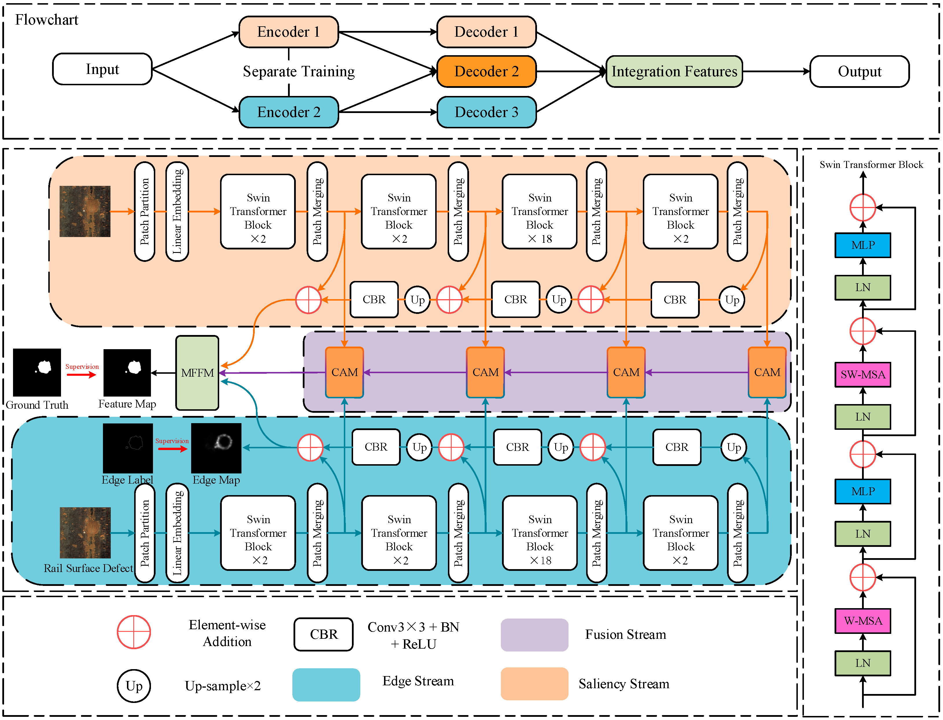
For the SOD of no-service rail surface detection, we propose a supervised deep learning network named TSSTNet and innovatively introduce the transformer as the backbone of the network;

(2)

A two-stream encoder and a three-stream decoder are proposed to eliminate the adverse effects between tasks;

(3)

A contour alignment module is presented to connect multitasking and reduce the noise at the edges of the saliency maps;

(4)

A multi-feature fusion module is proposed to converge the feature maps in the three different streams of the decoder;

(5)

We conducted a comparison experiment on the NRSD-MN [2] dataset with 10 SOTA methods [13,14,16,17,18,19,20,21,22,23]. The results indicate that our network performs better than the other networks on five metrics.

2. Related Works

2.1. Detection of Rail Defects

Rail defect detection is an integral part of the rail production process. Conventional non-destructive detection methods include magnetic particle detection, radiographic detection, eddy current detection, and ultrasonic detection. Antipov et al. [24] performed 3D computer simulations of magnetic flux leakage around transverse cracks in the rail head to detect the main characteristics of defects. Jian et al. [25] came up with an AE-signal-based detection system to detect defects by comparing the time intervals of AE wavelets. Mehel-Saidi et al. [26] proposed a method using a non-contact eddy current sensor to identify the different noises at the defect. Shi et al. [27] proposed a guided wave mode selection, which locates defects based on the different sensitivity of different modes to defects at various locations.

Meanwhile, neural-network-based vision algorithms are also popular in the field of rail defect detection. Zhang et al. [28] proposed a dual-stream neural network—one stream for generating samples and the other for classification. Zhang et al. [29] proposed an improved single-shot multibox detector (SSD) and You Only Look Once version 3 (YOLOv3), implementing the use of two networks to identify three different types of defects in parallel. Meng et al. [30] proposed a neural network framework for multitask learning to aid in track crack detection through track object detection.

2.2. Saliency Detection in RGB Images

Saliency detection, as the first step of many visual tasks, is growing in importance. It uses a computer vision algorithm and neural network learning to locate the most “remarkable” areas of the image. It helps people to highlight the areas of the image that should receive the most focus.

U-Net [31] effectively combines multilevel features using its unique U-shaped structure and skipping connection, making it the basic structure of most networks. EGNet [32] incorporates a model that obtains boundary information using low-level and high-level features, and then models the boundary information and target information. PiCANet [33] consists of an attention mechanism using pixel-wise contextual messages to learn location information for each pixel. Pyramid-Feature-Attention Network [34] consists of a context-aware pyramid feature extraction approach. U2Net [35] consists of a two-level nested U-structure and a residual U-block to capture more contextual information from different scales. ASNet [36] consists of an attention mechanism to imitate human visual attention mechanisms. CAGNet [37] consists of a feature guidance network to reduce the impacts of “salient like” appearance. PoolNet [38] consists of a global guidance module using different-sized pooling kernels to capture local and global information.

2.3. Contour Information Learning

Contour information as a separator between the foreground and background is important in saliency detection. Adding contour information to the network can significantly increase the effectiveness of saliency detection. The contour map can also refine the pixel distribution between the foreground and background. Contour detection is also increasingly being studied as a separate task.

CTDNet [12] consists of a trilateral decoder with spatial, semantic, and boundary paths. C2SNet [13] tries to graft a new branch onto a well-trained contour detection network and combines the contour task with the saliency task. PsiNet [14] consists of a structure with three parallel encoders, and one of them is used to perform the auxiliary tasks of contour detection. ENFNet [39] consists of a novel edge-guided structure to solve the problem of blurred edges caused by pooling operations.

2.4. Transformer

Bahdanau et al. [39] first applied an attention mechanism to the field of NLP. Vaswani et al. [40] first proposed a pure transformer, completely abandoning network structures such as traditional RNNs and CNNs. The transformer contains only the attention mechanism but achieves good results. After that, ViT [10] was proposed to use attention in the field of image processing. This approach splits the input image into several patches and sends them to transformer-like word vectors. Today, more and more transformers are being proposed to solve image classification, semantic segmentation and so on.

T2T [41] introduced tokens to tokens, enabling it to perform better on small datasets. DeiT [42] distills knowledge based on tokens, enabling it to perform better without pre-training on large datasets. Swin Transformer [11] consists of a multi-head self-attention mechanism based on shifted windows. PVT [43] consists of a shrinking pyramid and can contribute to downstream tasks, similar to the ResNet [44] backbone. CvT [45] combines the advantages of CNNs and transformers. It has both the dynamic attention mechanism and global modelling capabilities of transformers and the local capture capabilities of CNNs.

3. Methodology

3.1. Overview of the TSSTNet Framework

The proposed network TSSTNet is displayed in Figure 4. It comprises a two-stream encoder and a three-stream decoder. A contour alignment module (CAM) and a contour enhancement module (CEM) are proposed to use contour information learned by the edge stream to assist with saliency detection tasks. A feature fusion module (FFM) and a multi-feature fusion module (MFFM) are proposed to incorporate multi-model features. The details of the above four modules are showcased in Figure 5.

Specifically, the images are fed into two separately trained encoders after preprocessing, i.e., the edge stream and the saliency stream. Afterwards, the obtained features are fed into three different decoders—namely, the edge stream, the saliency stream, and the fusion stream—and the features from the three decoders are finally fused and output by the MFFM. The details are presented below.

3.2. Two-Stream Encoder and Three-Stream Decoder

In our experiments, we found that when using a single-stream encoder to perform multitask learning, the secondary task may interfere with the primary mission. Therefore, in our network, we propose a two-stream decoder—one stream for extracting features, and the other for boundary information. Separate training parameters are used for the two streams. The experimental results prove that the two-stream encoder works better than the single-stream encoder.

We propose a three-stream decoder consisting of a saliency stream (SS), edge stream (ES), and fusion stream (FS). It makes full use of the extracted multilevel feature maps. Features from stage i can be denoted as {S_i}${}_i^4$ in the SS, {E_i}${}_i^4$ in the ES, and {F_i}${}_i^4$ in the FS. The features in the SS and ES are then fused hierarchically by upsampling, convolution with a 3 × 3 kernel, batch normalization, and the ReLU activation function. At the same time, the CAM transfers the edge information learned from the ES to the SS by calculating the spatial position relationships, resulting in a precise contour. The three-stream decoder can be described as follows:

$$\left\{\begin{array}{l}{S}_i=CBR(Up(S_{i-1}))+S_i\\ E_i=CBR(Up(E_{i-1}))+E_i\end{array}\right.$$

(1)

$$F_i=CAM(S_i,E_i)+F_{i-1}$$

(2)

$$Result=MFFM(S_4,E_4,F_4)$$

(3)

where CBR denotes the 3 × 3 convolution, batch normalization, and ReLU function, while Up represents upsampling × 2.

3.3. Swin Transformer Backbone

Transformers increasingly perform better than CNNs on a wide range of visual tasks. Swin Transformer [11] not only retains the advantages of the ViT [10]—such as versatility, the ability to model the global long-range dependency features, and parallel processing capability—but also incorporates CNNs’ advantages of translational invariance and localization. Meanwhile, Swin Transformer [11] effectively solves the problem of heavy calculation caused by the self-attention operation. The contents of the Swin Transformer [11] are presented in Figure 4.

Specifically, Swin Transformer [11] firstly divides the RGB image into some non-overlapping patches via a patch partition operation, and then it applies a linear embedding layer on the patches, which transforms the data to a specific channel using a fully connected layer. After that, the patches are put into two successive Swin Transformer [11] blocks to extract multilevel features. The structure of the blocks is illustrated in Figure 4. With the network growing deeper, patch merging layers perform downsampling operations and reduce the resolution. Finally, we can capture the feature maps with the size of H/32, W/32, where H × W is the shape of the defect pictures. We chose Swin-B [11] as the pre-trained model in our network. Specifically, the fully connected layer converts the number of channels in the input patches to 128, while the number of repetitions of Swin Transformer [11] blocks is {2, 2, 18, 2}.

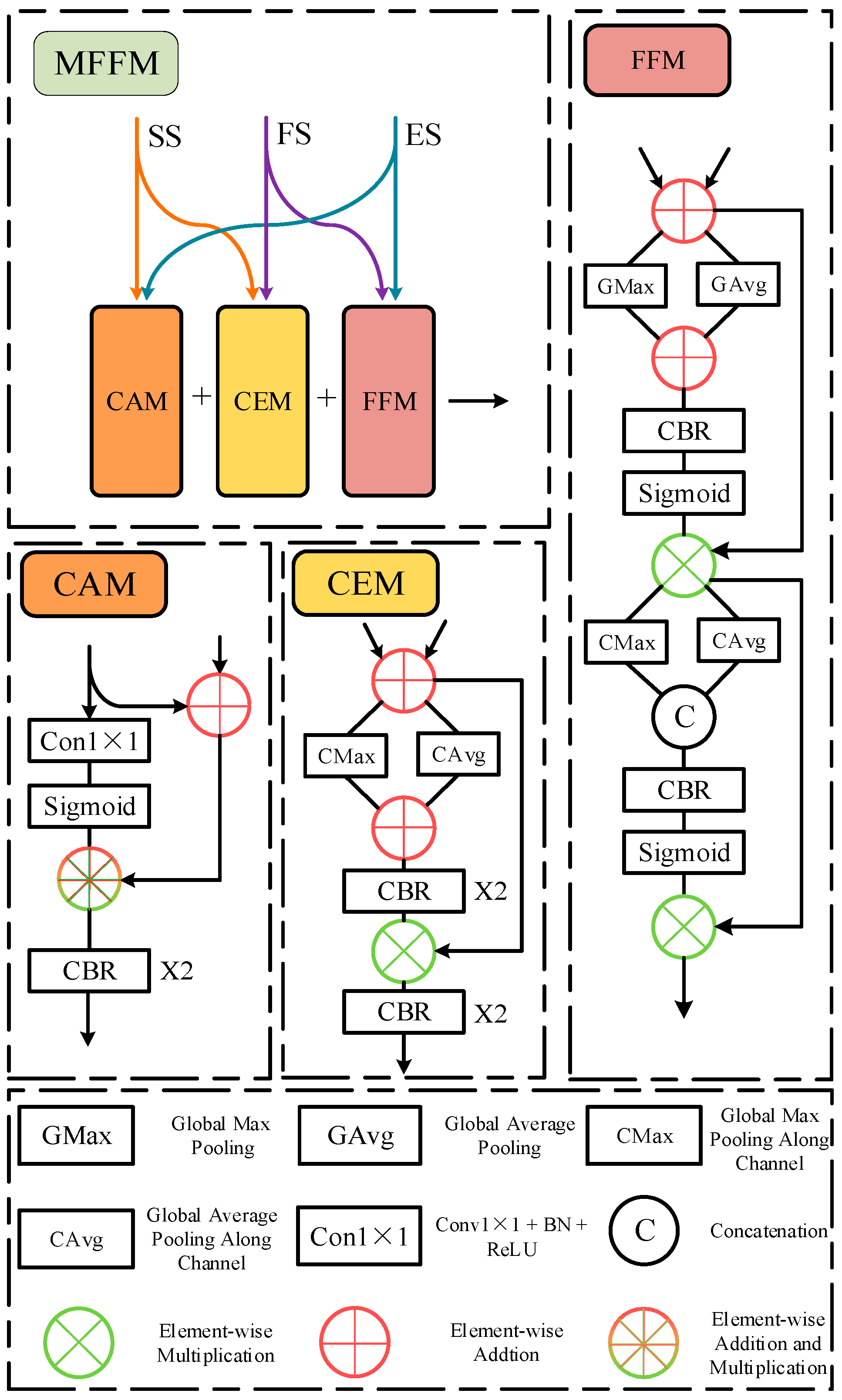
3.4. Multi-Feature Fusion Module

At the end of the network, we present a multi-feature fusion module (MFFM) that combines the features from the SS, ES, and FS two by two. For the multi-model maps in different streams, it contains three different models. These allow the network to learn boundary information while retaining the global context learned by the SS. The exact structures of the modules are described in more detail below, and the diagram of the structure of all modules is shown in Figure 5.

3.4.1. Contour Alignment Module

To use edge information to calibrate saliency detection, we propose a contour alignment module (CAM). We transform the edge map into probabilities of corresponding positions using the sigmoid function. Then, we align the edges of the rail defects by multiplying the saliency maps and the contour maps to deepen the image edges and reduce the noise between the background and foreground.

Specifically, we first merge the edge and the saliency maps by addition to form the fusion maps, and then we calculate the contour attention using a 1 × 1 convolution and sigmoid function. Then, we multiply and add the contour attention and the fusion map. Finally, two CBR functions are used to increase the learnability and complexity. Through contour attention, we expect the network to be more attentive to the edges of rail defects so as to achieve higher accuracy. The overall framework is shown in Figure 5. It can be formulized as follows:

$$CB{R}^2(x)=CBR(CBR(x))$$

(4)

$$CGM(S_i,E_i)=CB{R}^2\left[Sig(Cov1(E_i))\ast (E_i+S_i)+(E_i+S_i)\right]$$

(5)

where Cov1 denotes 1 × 1 convolution, Sig represents the sigmoid function, * denotes element-wise multiplication, and CBR² denotes two consecutive CBR functions.

3.4.2. Contour Enhancement Module and Feature Fusion Module

To combine the features in the ES and FS, we propose a contour enhancement module. Considering that the CAM aligns the contour maps to the saliency maps, we expect to let the edge maps guide the fine-tuning of the fusion maps through channel attention. Channel attention can improve the feature presentation of feature maps, while simultaneously reducing the noise at the edges of the feature maps due to the blurring of the edge maps. CEM can be presented as follows:

$$f_i=E_i+F_i$$

(6)

$$CEM(f_i)=CB{R}^2\left[CB{R}^2(CMax(f_i)+CAvg(f_i))\ast f_i\right]$$

(7)

where CMax represents the global max pooling operation along the channels, CAvg represents the global average pooling along the channels, and f_i is an intermediate feature. In this model, the contour on the feature is enhanced again.

Inspired by [46], we propose FFM by combining channel attention and spatial attention. However, we remove the bottleneck structure of the MLP in order to reduce the amount of computation in the network. We expect the fusion maps to pass contour information to saliency maps, while the saliency maps can retain semantic context information in the fusion maps. FFM can be denoted as follows:

$$S\_A=Sig(CBR(GMax(S_i+F_i)+GAvg(S_i+F_i)))\ast (S_i+F_i)$$

(8)

$$FFM(f_i)=Sig(CBR(Cat(CMax(S\_A),CAvg(S\_A))))\ast S\_A$$

(9)

where GMax denotes the global max pooling operation along the axis, GAvg denotes the global average pooling operation along the axis, S_A represents spatial attention, and Cat represents concatenation.

3.5. Training

We chose the NRSD-MN [2] dataset to train, validate, and test our network. The input size was processed to 384 × 384 × 3. This also corresponds to the input size of Swin-B. We enhanced the data using random flipping, rotation, and border clipping. Swin-B was chosen to initialize the parameters of the network. The batch size was programmed to 8, and the training epochs were set at 50. An Adam optimizer was introduced to train our network. The learning rate was initialized to 5 × 10⁻⁵, and then it decayed to 5 × 10⁻⁶ when the number of training epochs reached 30. We set the gradient clipping margin to 0.5. TSSTNet was trained on a machine with a single NVIDIA RTX 3090 and 24 GB graphics memory, and the approximate training time was 6 h. All code was implemented in the PyTorch framework.

4. Experimental Section

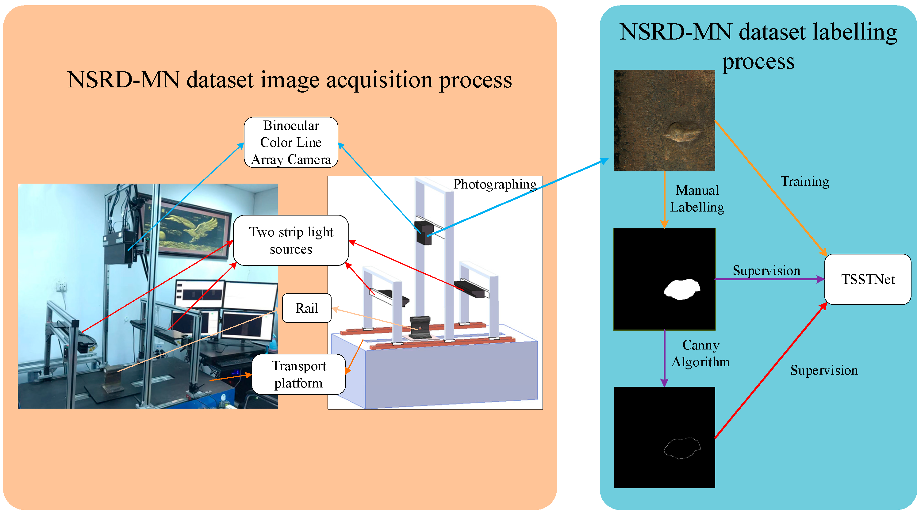
4.1. Datasets

To train TSSTNet, we selected the NSRD-MN [2] dataset. Zhang et al. [2] built a filming system consisting of a binocular color line-array camera, two light sources with a linear shape, and a motion transmission system. The color line-array camera reduces the light requirement to linear, uniform light. We used two linear light sources to provide linear uniform light. The camera cannot capture the entire surface of the rail at once, so a moving platform located underneath the rail carries the rail in slow motion. The specific structure is shown in Figure 6. The binocular line-array camera takes on the task of photographing. After the shoot, it manually annotates the images under the guidance of professionals from steel-testing companies. Then, we transform the annotations of the training and validation photos into edge annotations using the Canny [47] algorithm.

In summary, we obtained 3936 craft images of no-service rail surface defects (NRSDs), including 2158 images aged by a rust-promoting reagent, 1778 unaged pictures, and 165 natural NRSD photos. The natural set includes 115 highly similar and imitative images and 50 real images without any processing. They use metal to create scratches on the surface of the rails or use rust-promoting reagents on the surface of the metal to cause the metal to age and rust, making the manmade dataset look very similar to the natural one. The craft images were split into groups of 2086, 885, and 965 for training, validation, and testing, respectively, and the natural images were used as the test set.

4.2. Evaluation Metrics and Loss Function

To assess the capability of TSSTNet, we used five evaluation metrics commonly utilized in the field of SOD. Firstly, we chose the mean absolute error (MAE) [48] as our key metric, which visually shows the error between the predicted and true values. The formula is shown below:

$$MAE=\frac{1}{H\times W}{\displaystyle \sum _{j=1}^H{\displaystyle \sum _{k=1}^W|S(j,k)-G(j,k)|}}$$

(10)

where S is the saliency map, G is the ground truth (GT), j, k is the location of the pixel, and H × W is the size of the entry image.

The mean F-measure (mF_β) [49] was used to demonstrate the performance of the model by calculating Precision and Recall. The weighted F-measure (wF_β) was used to evaluate the positional accuracy of the salient results. Conventionally, we set β² to 0.3.

$$Precision=\frac{TP}{TP+FP}$$

(11)

$$Recall=\frac{TP}{TP+FN}$$

(12)

$$F_{\beta }=\frac{(1+{\beta }^2)\times Precision\times Recall}{{\beta }^2\times Precision\times Recall}$$

(13)

where TP means the true positive, FP means the false positive, and FN means the false negative in the contradiction matrix.

Structure-measure (S_α) [50] was used to measure the structural similarities between the predicted images and the annotations. There, we set α to 0.5.

$$S_{\alpha }=\alpha \ast S_o+(1-\alpha )\ast S_r$$

(14)

Enhanced-alignment measure (E_ξ) [51] focuses on the link between image-level data and local pixels by combining global pixel averages and local pixels. Finally, we also drew precision–recall (PR) and F-measure curves to show all information.

We choose binary cross-entropy loss (BCELoss) and intersection-over-union loss (IouLoss) as our loss functions. For training the edge maps, BCELoss was adopted as the edge stream loss (L_e).

$$L_e(P,G)=-\frac{1}{H\times W}{\displaystyle \sum _{j=1}^H{\displaystyle \sum _{k=1}^W\left[G(j,k)\ast log(P(j,k))+(1-G(j,k)\ast log(1-P(j,k))\right]}}$$

(15)

where G denotes the ground truth map, P denotes the prediction map, and j, k denotes the location of the pixel.

For training of the saliency maps, an integrated loss function (L_s) was introduced. In accordance with CTDNet [12], we set β to 0.6.

$$L_{iou}=1-\frac{{\displaystyle \sum _{j=1}^H{\displaystyle \sum _{k=1}^{W}G(j,k)P(j,k)}}}{{\displaystyle \sum _{j=1}^H{\displaystyle \sum _{k=1}^W\left[G(j,k)+P(j,k)-G(j,k)\times P(j,k)\right]}}}$$

(16)

$$L_s=\beta \times L_e+L_{iou}$$

(17)

As with the F-measure, we also chose PR curves to represent the relationship between precision and recall in the network results. Specifically, the precision and recall expressions indicate the percentage of true positives in the confusion matrix. The PR curve represents the relationship between precision and recall, and it is usually a convex curve. The higher the curve is to the right, the more effective the network. If two PR curves intersect, the further to the right the point is when P = R, the better the network.

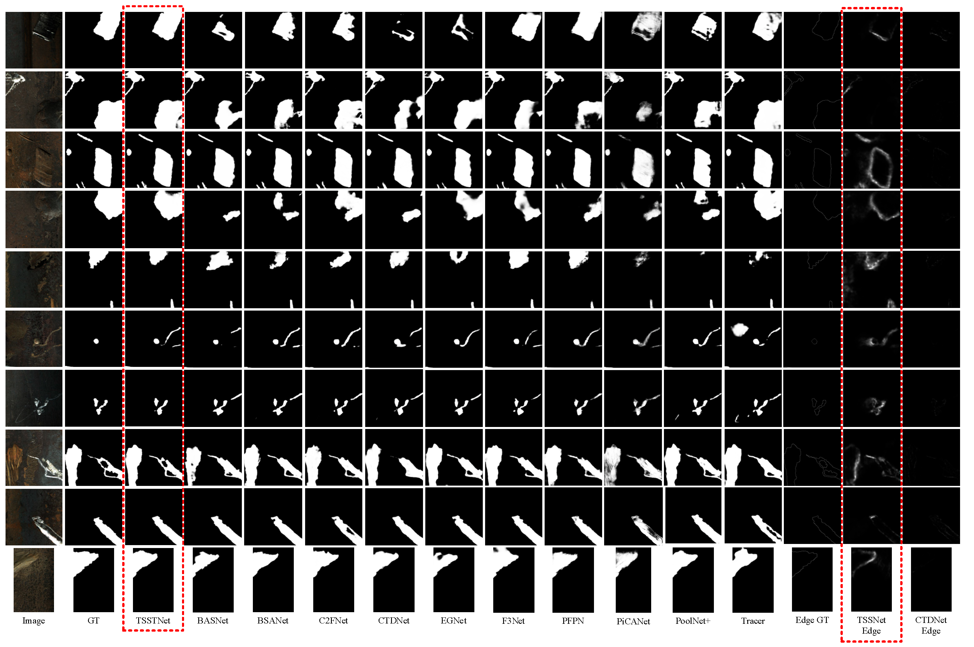
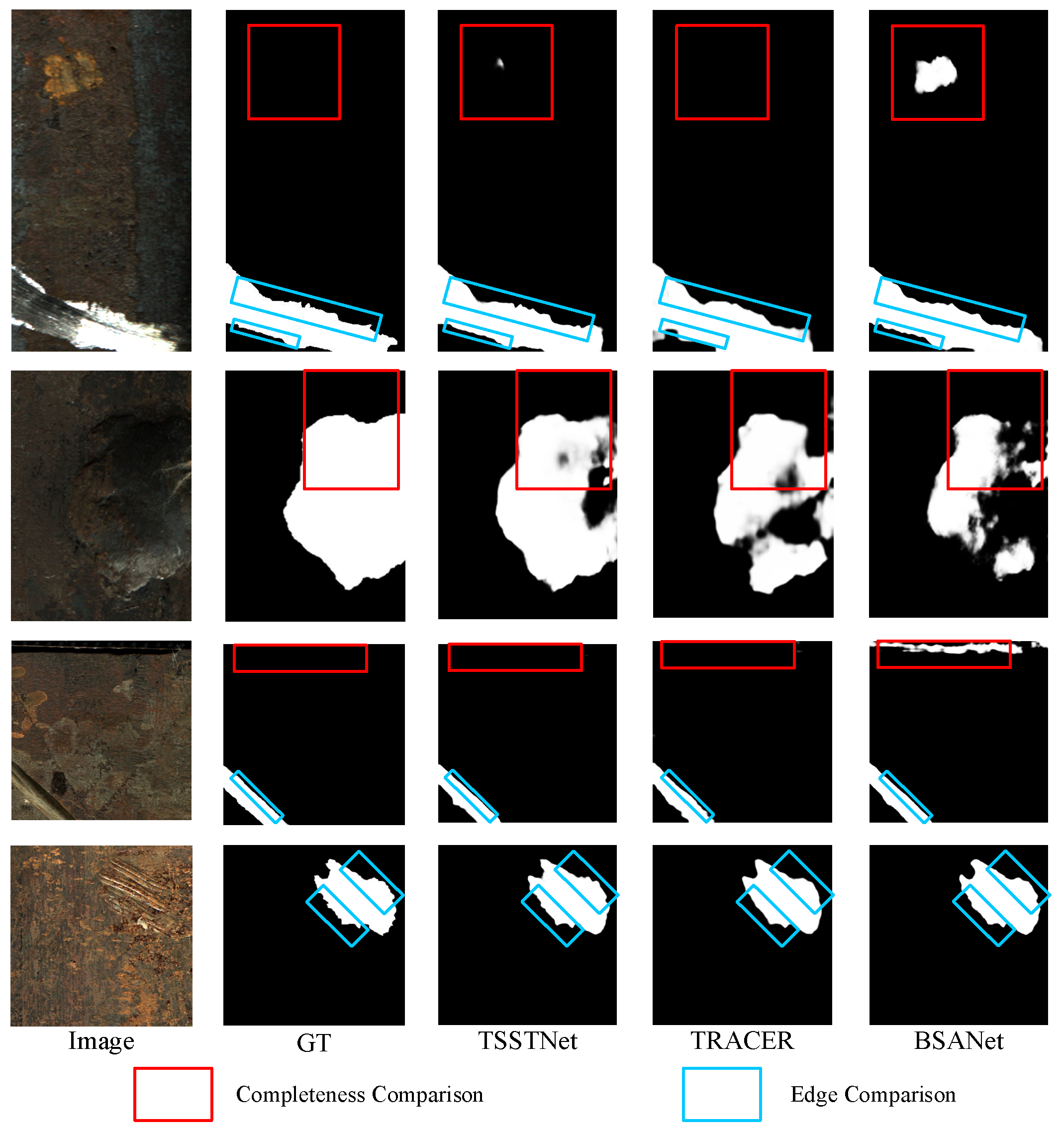
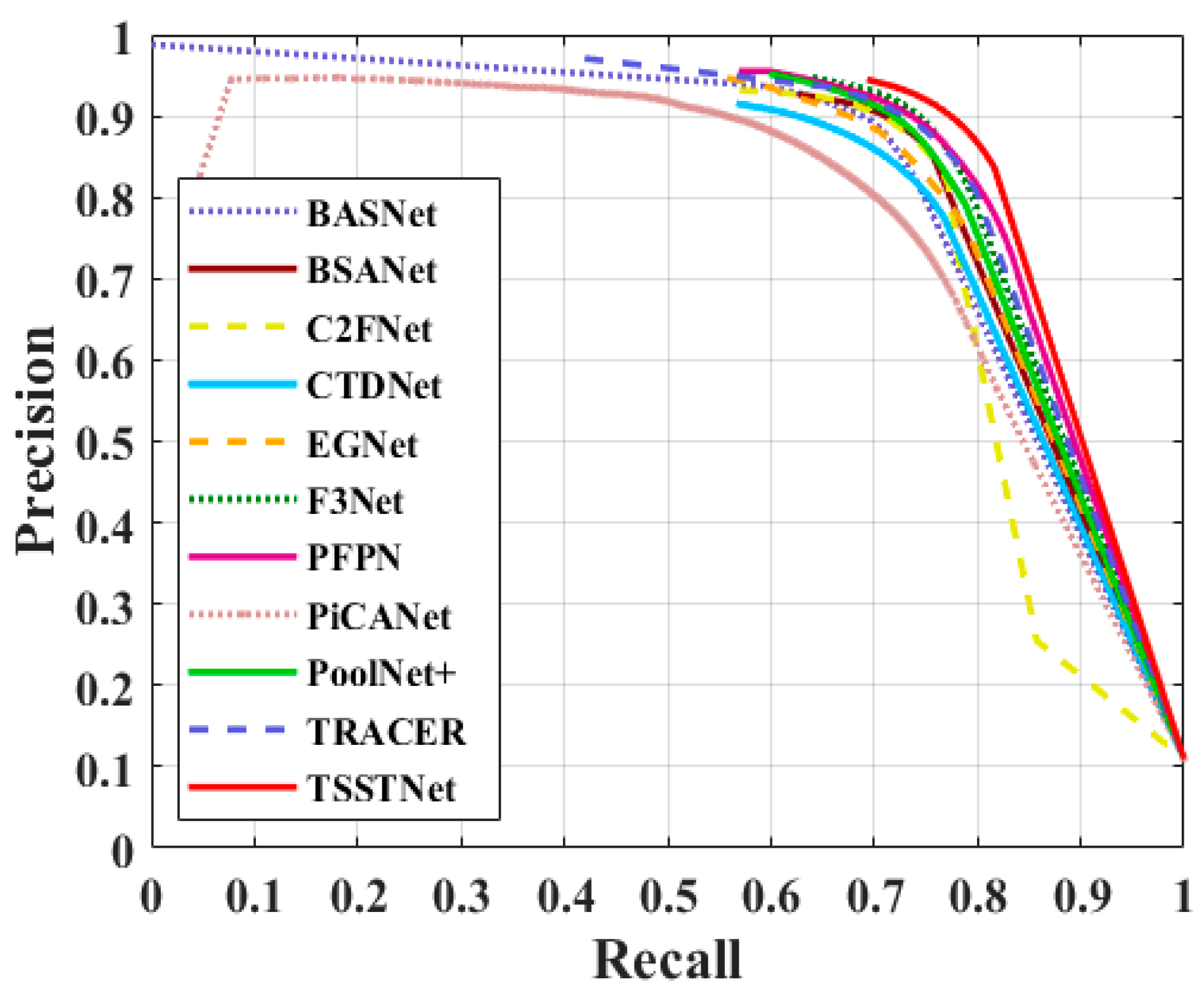
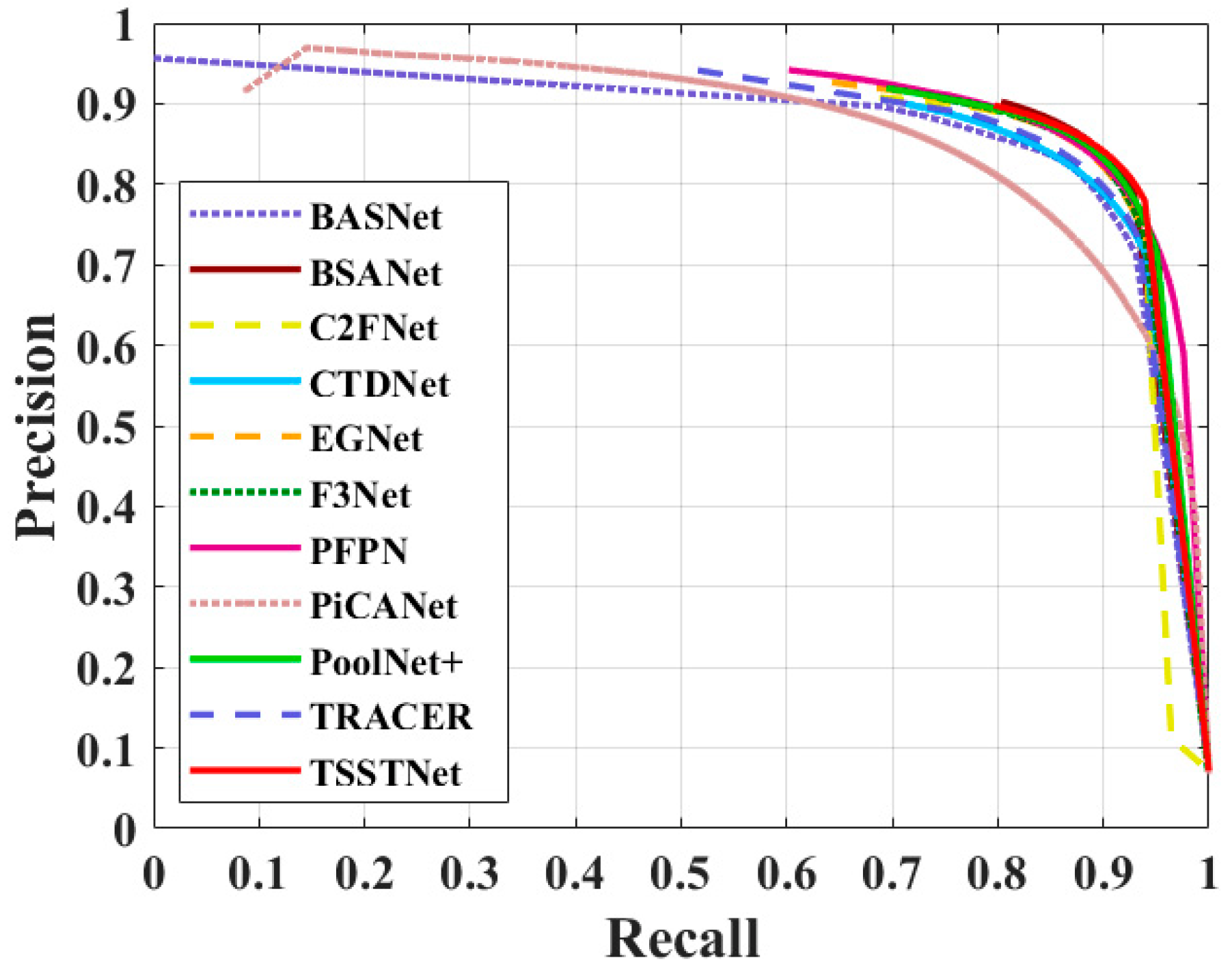
4.3. Comparison of Method Performance

We compared the performance of 10 SOTA deep learning neural networks widely used in SOD tasks on the NRSD-MN dataset (i.e., BASNet [44], BSANet [45], C2FNet [46], CTDNet [12], EGNet [24], F3Net [47], PFPN [48], PiCANet [25], PoolNet+ [49], and TRACER [51]). The results are shown in Figure 7, and we have marked the experimental results of TSSTNet with a dashed box. It can be clearly seen that the salient detection results obtained by our model are more accurate. Meanwhile, we compared the networks with similar test results in more detail. The comparative diagram is shown in Figure 8. In the diagram, we compare the visualization results in terms of detection completeness and edge refinement, using different-colored rectangular boxes to box them out. Benefiting from the edge stream, contour alignment module (CAM), and multi-feature fusion module (MFFM), we obtained a clearer contour. The code is available at https://github.com/VDT-2048/TSSTNet, which is accessed on 1 October 2022.

In terms of specific evaluation results, our network shows an improved effect compared to the latest proposed network TRACER [51], in the following ways: 0.6% lower MAE, 2.6% higher mF_β, 2.8% higher wF_β, 2.0% higher S_α, and 0.8% higher E_ξ on the natural surface defects dataset (Real); and 0.3% lower MAE, 3.7% higher mF_β, 3.6% higher wF_β, 1.4% higher S_α, and 1.2% higher for E_ξ on the manmade surface defects dataset (Craft). Other comparative results are illustrated in

Table 1. Comparison with 10 other common SOD networks; ↑ means the higher the better, ↓ means the lower the better. The best two results are tagged in red and green, respectively. MAE is the key metric.

Methods	NRSD-MN Dataset
	Real					Craft
	MAE ↓	mFβ ↑	wFβ ↑	Sα ↑	Eξ ↑	MAE ↓	mFβ ↑	wFβ ↑	Sα ↑	Eξ ↑
BASNet	0.065	0.748	0.730	0.797	0.830	0.021	0.802	0.775	0.866	0.944
BSANet	0.064	0.761	0.740	0.808	0.837	0.017	0.844	0.820	0.884	0.958
C2FNet	0.063	0.761	0.705	0.805	0.850	0.021	0.817	0.738	0.859	0.949
CTDNet	0.068	0.734	0.708	0.779	0.828	0.020	0.808	0.779	0.865	0.948
EGNet	0.063	0.746	0.723	0.798	0.840	0.019	0.814	0.797	0.872	0.948
F3Net	0.060	0.771	0.754	0.822	0.847	0.018	0.824	0.799	0.879	0.950
PFPN	0.059	0.759	0.742	0.819	0.857	0.019	0.798	0.793	0.871	0.940
PiCANet	0.076	0.679	0.633	0.749	0.826	0.031	0.718	0.695	0.819	0.901
PoolNet+	0.061	0.760	0.740	0.811	0.839	0.017	0.825	0.805	0.875	0.953
TRACER	0.058	0.772	0.753	0.819	0.859	0.019	0.825	0.805	0.875	0.953
Ours	0.052	0.798	0.781	0.839	0.867	0.016	0.841	0.816	0.883	0.958

.

The experimental results show that our network is highly competitive in saliency detection. Benefiting from the Swin Transformer [11] backbone and the two-stream multitasking encoder, our network is more accurate in feature extraction. At the same time, the CAM helps the network to distinguish between ambiguous foregrounds and backgrounds very well.

We drew PR curves and F-measure curves to show the relationship between precision and recall, as shown in Figure 9 and Figure 10, respectively. From the PR curve analysis, we can infer that TSSTNet performs much better than the other comparison networks on the real dataset. On the craft dataset, several networks achieved similar results, but TSSTNet was still superior to the other networks.

4.4. Ablation Experiments

To verify our conjecture about the benefits of two-stream networks, and to evaluate the advantages and disadvantages of the proposed modules, we conducted several ablation experiments. We used upsampling operations and element-wise addition to merge the hierarchical features to form a U-shaped structure. We also removed the MFFM and the FS separately using the control variable method. In the experiments to eliminate the MFFM, we used element-wise addition instead of the MFFM to fuse the ES, SS, and FS. The results of the investigation are displayed in

Table 2. Results of the ablation experiments; ↑ means the higher the better, ↓ means the lower the better. The best two results are tagged in red and green, respectively. MAE is the key metric.

	Swin Transformer Backbone	Two-Stream Encoder	Three-Stream Decoder	MFFM	NRSD-MN Dataset	MAE ↓	mFβ ↑	wFβ ↑	Sα ↑	Eξ ↑
Test1	√				Real	0.056	0.787	0.767	0.825	0.856
Test2	√	√				0.053	0.805	0.776	0.820	0.874
Test3	√	√	√			0.099	0.705	0.359	0.732	0.835
TSSTNet	√	√	√	√		0.052	0.798	0.781	0.839	0.867
Test4	√				Craft	0.017	0.831	0.807	0.880	0.955
Test5	√	√				0.020	0.833	0.810	0.860	0.954
Test6	√	√	√			0.062	0.761	0.389	0.771	0.921
TSSTNet	√	√	√	√		0.016	0.841	0.816	0.883	0.958

.

The experimental results indicate that the two-stream encoder can indeed solve the problem of the auxiliary task interacting with the main task in the single-stream encoder. Furthermore, the combination of the three-stream features extracted by the two-stream encoder through the MFFM can solve the problem of conflict when different features are fused.

5. Conclusions

In this paper, we present a multi-stream neural network named Two-Stream Swin Transformer Network (TSSTNet) to meet the challenge of blurring the edges of rail surface defects and distinguishing the foreground from the background. TSSTNet uses two separately trained encoders to extract saliency features and edge features, which is a good solution to the problem of inter-task interference when a single-stream encoder is working on multiple tasks. This also makes TSSTNet highly capable of edge refinement. At the same time, we propose a contour alignment module (CAM) to use spatial attention to fuse features from different streams, which calibrates the edges of the saliency detection map, reduces noise at the foreground–background junction, and helps the network to locate defects. Moreover, a multi-feature fusion module (MFFM) is proposed to solve the problem of conflicting features at different levels of the three-stream decoder, which is able to reduce the variability in the fusion of features learned from different streams. However, a dual-stream decoder with separately trained parameters would result in a larger model and more computational effort. In subsequent studies, we will remove the less important parts of the network by pruning, compression, and other operations to lighten the network. In addition to this, we will commit to the use of multimodal information—including RGB-D and RGB-T images [51]—for the detection of no-service rail surface defects.

References

1. Gan, J.; Li, Q.; Wang, J.; Yu, H. A hierarchical extractor-based visual rail surface inspection system. IEEE Sens. J. 2017, 17, 7935–7944. [Google Scholar] [CrossRef]
2. Zhang, D.; Song, K.; Xu, J.; He, Y.; Niu, M.; Yan, Y. MCnet: Multiple Context Information Segmentation Network of No-Service Rail Surface Defects. IEEE Trans. Instrum. Meas. 2021, 70, 1–9. [Google Scholar] [CrossRef]
3. Xu, P.; Zeng, H.; Qian, T.; Liu, L. Research on defect detection of high-speed rail based on multi-frequency excitation composite electromagnetic method. Measurement 2022, 187, 110351. [Google Scholar] [CrossRef]
4. Hao, F.; Shi, J.; Zhang, Z.; Chen, R.; Zhu, S. Canny edge detection enhancement by general auto-regression model and bi-dimensional maximum conditional entropy. Optik 2014, 125, 3946–3953. [Google Scholar] [CrossRef]
5. Cao, B.; Li, J.; Liu, C.; Qin, L. Defect detection of nickel plated punched steel strip based on improved least square method. Optik 2020, 206, 164331. [Google Scholar] [CrossRef]
6. Hao, Q.; Zhang, X.; Wang, Y.; Shen, Y.; Makis, V. A novel rail defect detection method based on undecimated lifting wavelet packet transform and Shannon entropy-improved adaptive line enhancer. J. Sound Vib. 2018, 425, 208–220. [Google Scholar] [CrossRef]
7. Shakeel, M.S.; Zhang, Y.; Wang, X.; Kang, W.; Mahmood, A. Multi-scale Attention Guided Network for End-to-End Face Alignment and Recognition. J. Vis. Commun. Image Represent. 2022, 88, 103628. [Google Scholar] [CrossRef]
8. Baffour, A.A.; Qin, Z.; Wang, Y.; Qin, Z.; Choo, K.K.R. Spatial self-attention network with self-attention distillation for fine-grained image recognition. J. Vis. Commun. Image Represent. 2021, 81, 103368. [Google Scholar] [CrossRef]
9. Borji, A.; Cheng, M.; Hou, Q.; Jiang, H.; Li, J. Salient object detection: A survey. Comput. Vis. Media 2019, 5, 117–150. [Google Scholar] [CrossRef] [Green Version]
10. Dosovitskiy, A.; Beyer, L.; Kolesnikov, A.; Weissenborn, D.; Zhai, X.; Unterthiner, T.; Dehghani, M.; Minderer, M.; Heigold, G.; Gelly, S.; et al. An image is worth 16x16 words: Transformers for image recognition at scale. arXiv 2020, arXiv:2010.11929. [Google Scholar]
11. Liu, Z.; Lin, Y.; Cao, Y.; Hu, H.; Wei, Y.; Zhang, Z.; Lin, S.; Guo, B. Swin transformer: Hierarchical vision transformer using shifted windows. In Proceedings of the IEEE/CVF International Conference on Computer Vision, Montreal, QC, Canada, 10–17 October 2021; pp. 10012–10022. [Google Scholar]
12. Zhao, Z.; Xia, C.; Xie, C.; Li, J. Complementary trilateral decoder for fast and accurate salient object detection. In Proceedings of the 29th ACM International Conference on Multimedia, Virtual, 20–24 October 2021; pp. 4967–4975. [Google Scholar]
13. Li, X.; Yang, F.; Cheng, H.; Liu, W. Contour knowledge transfer for salient object detection. In Proceedings of the European Conference on Computer Vision (ECCV), Munich, Germany, 8–14 September 2018; pp. 355–370. [Google Scholar]
14. Murugesan, B.; Sarveswaran, K.; Shankaranarayana, S.M.; Ram, K.; Joseph, J.; Sivaprakasam, M. Psi-Net: Shape and boundary aware joint multi-task deep network for medical image segmentation. In Proceedings of the 2019 41st Annual International Conference of the IEEE Engineering in Medicine and Biology Society (EMBC), Berlin, Germany, 23–27 July 2019; pp. 7223–7226. [Google Scholar] [CrossRef]
15. Tu, Z.; Ma, Y.; Li, C.; Tang, J.; Luo, B. Edge-guided non-local fully convolutional network for salient object detection. IEEE Trans. Circuits Syst. Video Technol. 2020, 31, 582–593. [Google Scholar] [CrossRef] [Green Version]
16. Zhang, J.; Li, S.; Yan, Y.; Ni, Z.; Ni, H. Surface Defect Classification of Steel Strip with Few Samples Based on Dual-Stream Neural Network. Steel Res. Int. 2022, 93, 2100554. [Google Scholar] [CrossRef]
17. Wu, H.; Xiao, B.; Codella, N.; Liu, M.; Dai, X.; Yuan, L.; Zhang, L. Cvt: Introducing convolutions to vision transformers. In Proceedings of the IEEE/CVF International Conference on Computer Vision, Montreal, QC, Canada, 10–17 October 2021; pp. 22–31. [Google Scholar]
18. Woo, S.; Park, J.; Lee, J.Y.; Kweon, I.S. Cbam: Convolutional block attention, module. In Proceedings of the European Conference on Computer Vision (ECCV), Munich, Germany, 8–14 September 2018; pp. 3–19. [Google Scholar]
19. Ding, L.; Goshtasby, A. On the Canny edge detector. Pattern Recognit. 2001, 34, 721–725. [Google Scholar] [CrossRef]
20. Willmott, C.J.; Matsuura, K. Advantages of the mean absolute error (MAE) over the root mean square error (RMSE) in assessing average model performance. Clim. Res. 2005, 30, 79–82. [Google Scholar] [CrossRef]
21. Achanta, R.; Hemami, S.; Estrada, F.; Susstrunk, S. Frequency-tuned salient region detection. In Proceedings of the 2009 IEEE Conference on Computer Vision and Pattern Recognition, Miami, FL, USA, 20–25 June 2009; pp. 1597–1604. [Google Scholar] [CrossRef] [Green Version]
22. Fan, D.P.; Cheng, M.M.; Liu, Y.; Li, T.; Borji, A. Structure-measure: A new way to evaluate foreground maps. In Proceedings of the IEEE International Conference on Computer Vision, Venice, Italy, 22–29 October 2017; pp. 4548–4557. [Google Scholar]
23. Fan, D.P.; Gong, C.; Cao, Y.; Ren, B.; Cheng, M.; Borji, A. Enhanced-alignment measure for binary foreground map evaluation. arXiv 2018, arXiv:1805.10421. [Google Scholar]
24. Antipov, A.G.; Markov, A.A. Detectability of Rail Defects by Magnetic Flux Leakage Method. Russ. J. Nondestruct. Test. 2019, 55, 277–285. [Google Scholar] [CrossRef]
25. Jian, H.; Lee, H.R.; Ahn, J.H. Detection of bearing/rail defects for linear motion stage using acoustic emission. Int. J. Precis. Eng. Manuf. 2013, 14, 2043–2046. [Google Scholar] [CrossRef]
26. Mehel-Saidi, Z.; Bloch, G.; Aknin, P. A subspace method for detection and classification of rail defects. In Proceedings of the 2008 16th European Signal Processing Conference, Lausanne, Switzerland, 25–29 August 2008; pp. 1–5. [Google Scholar]
27. Shi, H.; Zhuang, L.; Xu, X.; Yu, Z.; Zhu, L. An Ultrasonic Guided Wave Mode Selection and Excitation Method in Rail Defect Detection. Appl. Sci. 2019, 9, 1170. [Google Scholar] [CrossRef] [Green Version]
28. Zhang, H.; Song, Y.; Chen, Y.; Zhong, H. MRSDI-CNN: Multi-model rail surface defect inspection system based on convolutional neural networks. IEEE Trans. Intell. Transp. Syst. 2021, 23, 11162–11177. [Google Scholar] [CrossRef]
29. Meng, S.; Kuang, S.; Ma, Z.; Wu, Y. MtlrNet: An Effective Deep Multitask Learning Architecture for Rail Crack Detection. IEEE Trans. Instrum. Meas. 2022, 71, 1–10. [Google Scholar] [CrossRef]
30. Ronneberger, O.; Fischer, P.; Brox, T. U-net: Convolutional networks for biomedical image segmentation. In Proceedings of the International Conference on Medical Image Computing and Computer-Assisted Intervention, Munich, Germany, 5–9 October 2015; Springer: Cham, Switzerland, 2015; pp. 234–241. [Google Scholar]
31. Zhao, J.X.; Liu, J.J.; Fan, D.P.; Cao, Y. EGNet: Edge guidance network for salient object detection. In Proceedings of the IEEE/CVF International Conference on Computer Vision, Seoul, Korea, 27 October–November 2019; pp. 8779–8788. [Google Scholar]
32. Liu, N.; Han, J.; Yang, M.H. Picanet: Learning pixel-wise contextual attention for saliency detection. In Proceedings of the IEEE conference on computer vision and pattern recognition, Salt Lake City, UT, USA, 18–23 June 2018; pp. 3089–3098. [Google Scholar]
33. Zhao, T.; Wu, X. Pyramid feature attention network for saliency detection. In Proceedings of the IEEE/CVF Conference on Computer Vision and Pattern Recognition, Long Beach, CA, USA, 16–27 June 2019; pp. 3085–3094. [Google Scholar]
34. Qin, X.; Zhang, Z.; Huang, C.; Dehghan, M.; Zaiane, O.R. U2-Net: Going deeper with nested U-structure for salient object detection. Pattern Recognit. 2020, 106, 107404. [Google Scholar] [CrossRef]
35. Zhu, L.; Feng, S.; Zhu, W.; Chen, X. ASNet: An adaptive scale network for skin lesion segmentation in dermoscopy images. In Medical Imaging 2020: Biomedical Applications in Molecular, Structural, and Functional Imaging; SPIE: Bellingham, WA, USA, 2020; Volume 11317, pp. 226–231. [Google Scholar]
36. Mohammadi, S.; Noori, M.; Bahri, A.; Majelan, S.G. CAGNet: Content-aware guidance for salient object detection. Pattern Recognit. 2020, 103, 107303. [Google Scholar] [CrossRef] [Green Version]
37. Liu, J.J.; Hou, Q.; Cheng, M.M. A simple pooling-based design for real-time salient object detection. arXiv 2019, arXiv:1904.09569. [Google Scholar]
38. Bahdanau, D.; Cho, K.; Bengio, Y. Neural machine translation by jointly learning to align and translate. arXiv 2014, arXiv:1409.0473. [Google Scholar]
39. Vaswani, A.; Shazeer, N.; Parmar, N.; Uszkoreit, J.; Jones, L.; Gomez, A.N.; Kaiser, L.; Polosukhin, I. Attention is all you need. Adv. Neural Inf. Process. Syst. 2017, 30. Available online: https://proceedings.neurips.cc/paper/2017/file/3f5ee243547dee91fbd053c1c4a845aa-Paper.pdf (accessed on 7 October 2022).
40. Yuan, L.; Chen, Y.; Wang, T.; Yu, W.; Shi, Y.; Jiang, Z.; Tay, F.E.H.; Feng, J.; Yan, S. Tokens-to-token vit: Training vision transformers from scratch on imagenet. In Proceedings of the IEEE/CVF International Conference on Computer Vision, Montreal, QC, Canada, 11–17 October 2021; pp. 558–567. [Google Scholar]
41. Touvron, H.; Cord, M.; Douze, M.; Massa, F.; Sablayrolles, A.; Jegou, H. Training data-efficient image transformers & distillation through attention. In Proceedings of the 38th International Conference on Machine Learning, PMLR 2021, Virtual, 18–24 July 2021; Volume 139, pp. 10347–10357. [Google Scholar]
42. Wang, W.; Xie, E.; Li, X.; Fan, D.; Song, K.; Liang, D.; Lu, T.; Luo, P. Pyramid vision transformer: A versatile backbone for dense prediction without convolutions. In Proceedings of the IEEE/CVF International Conference on Computer Vision, Montreal, QC, Canada, 11–17 October 2021; pp. 568–578. [Google Scholar]
43. He, K.; Zhang, X.; Ren, S.; Sun, J. Deep residual learning for image recognition. In Proceedings of the IEEE Conference on Computer Vision and Pattern Recognition, San Francisco, CA, USA, 18–20 June 2016; pp. 770–778. [Google Scholar]
44. Qin, X.; Zhang, Z.; Huang, C.; Gao, C.; Dehghan, M.; Jagersand, M. Basnet: Boundary-aware salient object detection. In Proceedings of the IEEE/CVF Conference on Computer Vision and Pattern Recognition, Long Beach, CA, USA, 16–17 June 2019; pp. 7479–7489. [Google Scholar]
45. Zhu, H.; Li, P.; Xie, H.; Yan, X.; Liang, D.; Chen, D.; Wei, M.; Qin, J. I can find you! Boundary-guided Separated Attention Network for Camouflaged Object Detection. AAAI 2022. Available online: https://ojs.aaai.org/index.php/AAAI/article/view/20273 (accessed on 7 October 2022).
46. Sun, Y.; Chen, G.; Zhou, T.; Zhang, Y.; Liu, N. Context-aware cross-level fusion network for camouflaged object detection. arXiv 2021, arXiv:2105.12555. [Google Scholar]
47. Wei, J.; Wang, S.; Huang, Q. F3Net: Fusion, feedback and focus for salient object detection. In Proceedings of the AAAI Conference on Artificial Intelligence 2020, New York, NY, USA, 7–12 February 2020; Volume 34, pp. 12321–12328. [Google Scholar]
48. Wang, B.; Chen, Q.; Zhou, M.; Zhang, Z.; Jin, X.; Gai, K. Progressive feature polishing network for salient object detection. In Proceedings of the AAAI Conference on Artificial Intelligence 2020, New York, NY, USA, 7–12 February 2020; Volume 34, pp. 12128–12135. [Google Scholar]
49. Liu, J.; Hou, Q.; Liu, Z.; Cheng, M. PoolNet+: Exploring the Potential of Pooling for Salient Object Detection. In IEEE Transactions on Pattern Analysis and Machine Intelligence; IEEE: Piscataway, NJ, USA, 2022. [Google Scholar] [CrossRef]
50. Lee, M.S.; Shin, W.S.; Han, S.W. TRACER: Extreme Attention Guided Salient Object Tracing Network (Student Abstract). In Proceedings of the AAAI Conference on Artificial Intelligence, Pomona, CA, USA, 24–28 October 2022; Volume 36, pp. 12993–12994. [Google Scholar]
51. Song, K.; Wang, J.; Bao, Y.; Huang, L.; Yan, Y. A Novel Visible-Depth-Thermal Image Dataset of Salient Object Detection for Robotic Visual Perception. In IEEE/ASME Transactions on Mechatronics; IEEE: Piscataway, NJ, USA, 2022. [Google Scholar] [CrossRef]
Figure 1. (a) Surface view of an in-service rail with defects [1]. (b) Surface view of an in-service rail [1]. (c) Surface view of a no-service rail with defects [2]. (d) Surface view of a no-service rail [2].
Coatings 12 01730 g001
Figure 2. (a) Rail defect map. (b) Single Swin Transformer saliency map. (c) Ground truth (d) TSSTNet saliency map.
Coatings 12 01730 g002
Figure 3. (a) No-service rail surface defects. (b) Edge ground truth. (c) Contour maps of TSSTNet. (d) Contour maps of CTDNet [12].
Coatings 12 01730 g003
Figure 4. Structural diagrams of our proposed network TSSTNet.
Coatings 12 01730 g004
Figure 5. Structural diagrams of the contour alignment module (CAM), contour enhancement module (CEM), feature fusion module (FFM), and multi-feature fusion module (MFFM).
Coatings 12 01730 g005
Figure 6. The process of creating the NSRD-MN dataset.
Coatings 12 01730 g006
Figure 7. Visualized saliency maps of no-service rail surface defect detection compared with 10 other networks.
Coatings 12 01730 g007
Figure 8. Visual comparison of the two networks with the most similar test results from detection of completeness and edge refinement.
Coatings 12 01730 g008
Figure 9. PR curves for the real NRSD-MN dataset.
Coatings 12 01730 g009
Figure 10. PR curves for the craft NRSD-MN dataset.
Coatings 12 01730 g010