A Semi-Supervised Inspection Approach of Textured Surface Defects under Limited Labeled Samples

Abstract

Defect inspection is a key step in guaranteeing the surface quality of industrial products. Based on deep learning (DL) techniques, related methods are highly effective in defect classification tasks via a supervision process. However, collecting and labeling many defect samples are usually harsh and time-consuming processes, limiting the application of these supervised classifiers on various textured surfaces. This study proposes a semi-supervised framework, based on a generative adversarial network (GAN) and a convolutional neural network (CNN), to classify defects of a textured surface, while a novel label assignment scheme is proposed to integrate unlabeled samples into semi-supervised learning to enhance the overall performance of the system. In this framework, a customized GAN uses limited labeled samples to generate unlabeled ones, while the proposed label assignment scheme makes the generated data follow different label distributions in such a way that they can participate in training with labeled data. Finally, a CNN is proposed for semi-supervised training and the category identification of each defect sample. Experimental results show the effectiveness and robustness of the proposed framework even if original samples are limited. We verify our approach on four different surface defect datasets, achieving consistently competitive performances.

1. Introduction

Defect classification is a fundamental industrial inspection task, the aim of which is to identify the category of a defective image. It is commonly performed on textured surfaces of many industrial products, such as metal [1], wood [2], and fabrics [3,4,5]. This process is crucial to guarantee product quality but is always executed manually in practice. Aiming at replacing this human-involved operation, there are many approaches using machine learning or deep learning techniques in automatic defect classification. However, these methods are mainly based on a supervised scenario, where all the data must be labeled. Unfortunately, the defect samples not only are hard to collect in large numbers but also need to be labeled by experts. Supervised approaches have no ability to handle unlabeled samples, which can lead to defect misclassification. This work introduces a semi-supervised learning (SSL) approach that can generate and handle unlabeled defect data in such a way that outperforms the supervised ones which only deal with labeled data. Therefore, the SSL approach can achieve reliable accuracy with limited samples, and the heavy and complicated manual sample collection and label allocation work can be alleviated.

To achieve automatic defect classification, the previous work on addressing this problem can be categorized into traditional shallow network learning (SNL)-based approaches and deep network learning (DNL)-based approaches. For simplicity, they are called SNL-based and DNL-based approaches, respectively.

SNL-based methods: In [6], Zhang et al. extracted the features based on Fisher distance and principal component analysis (PCA), and used the support vector machine (SVM) classifier for defect detection on an aluminum alloy surface. Yunwon and Kweon [7] proposed a neighboring difference filter algorithm to extract the foreground defective regions and used a random forest for defect classification. In [8], a guidance template-based algorithm using the statistical characteristic of textures is proposed for defect classification of strip steel surface. In [9], the combination of the completed local binary pattern (CLBP) features and the nearest-neighbor classifier are used to perform defect classification tasks. It is noteworthy that studies [7,8,9] are the combination of a hand-crafted feature extractor and a typical ML classifier, which highly rely on human experience.

DNL-based methods: Zhou et al. [10] used a simple sequential structured CNN for feature extraction and fed the representation tensors into a softmax layer for classification. Hossain et al. [11] proposed a light model of a six-layer CNN for fruit classification. Huang et al. [12] designed a small FCN network a quarter of the size of the original network [13]. These methods usually had to use tiny CNN structures because of limited industrial data. Except for the self-designed networks, some approaches adopted various baseline CNNs for defect classification via transfer learning. Through pre-training on the large dataset ImageNet, large baseline CNNs with dozens of layers, such as AlexNet [14], VGG [15], Inception [16], and ResNet [17], can be applied to specific tasks and avoid over-fitting. In [11], the classification system used not only a tiny model but also fine-tuned a pre-trained VGG16 model. Studies [18,19] directly used pre-trained models for representation learning and then fine-tuned them by their own data for defect classification. The approach presented in [18] used the ZFNet to classify various textured surface defects and gave further evidence that ImageNet pre-trained models can be applied in industrial inspection tasks, whereas the distributions of textured defect data differ from those of ImageNet data. Yang et al. in [19] presented the transfer learning method for surface defect classification of flat panel displays. The study used AlexNet as the backbone and reduced one fully connected layer for online training. Using large models can achieve higher precision but also cost more computation sources because of many model parameters, especially in the last fully connected layers. Therefore, some approaches combined the DL and ML techniques, which regarded the convolutional part as a feature extractor, with the aim to replace hand-crafted features, and then are fed into a typical ML classifier. Studies [12,20] combined the transferred CNN features and various ML classifiers in pursuit of a more economical inspection system. Natarajan et al. in [20] used a combination of the VGG [15] model and the SVM classifier for metal surface defect classification, where VGG was employed to extract feature maps which were then used as input to SVM. In [12], hierarchies of features were extracted by FCN models and a two-stream algorithm was proposed to classify defects, which can only be applied on single-class image. The combination-like strategy aims to replace hand-crafted features with CNN features, which have a higher abstract level and stronger robustness [21]. However, this also resulted in poor generalization and an extra training process for the ML classifier. The main drawback of the previous approaches is that they highly depend on supervised learning, which requires enough defect samples and can only process labeled ones. The above approaches, whether based on fully supervised learning or transfer learning, all fail to provide correct classification in the presence of unlabeled samples.

Therefore, this study attempts to establish an SSL defect classification system, which can handle both labeled and unlabeled samples. Indeed, for an SSL scheme, the first consideration is the acquisition of unlabeled samples. As in other fields [22,23,24], the semi-supervised or weakly supervised learning methods can work on enough unlabeled samples that have become available on the Internet. However, it seems impossible to collect the same scale of defect data due to the rare occurrence of defects and the privatization of available data. Therefore, it is a better choice to consider how to generate valuable samples instead of taking much time to collect real ones. In this paper, a standard generative adversarial network (GAN) architecture is customized to fit defect data and then used to generate unlabeled samples [25]. Based on original defect samples, the GAN can generate new ones through a competitive training process involving a pair of networks.

When there are enough unlabeled samples, the second problem is how to include them in training. Different from transfer learning that trains labeled and unlabeled samples alternately, the SSL system needs to train both simultaneously. The unlabeled samples are often assigned to weak or pseudo labels for SSL, which is not a good choice for GAN samples. The unlabeled samples they used, such as in studies [23,26], are real but GAN samples are fake data generated by training. The existing methods of processing GAN samples are too rough, treating them the same way during training—the GAN samples are regarded as an extra class [27] or placed directly into existing classes [28].

We consider that all the GAN samples cannot be regarded as identical; the high-quality ones should be used to expand the original dataset and the low-quality ones can boost the learning process but not affect its optimization direction. This study proposes the label assignment for the unlabeled samples (LAUS) algorithm, which makes different assumptions for the unlabeled samples. The high-quality samples regarded as real images are assigned the corresponding ground-truth class distributions, and the low-quality ones are assigned a uniform label distribution over all the ground-truth classes, which assumes that these samples do not belong to a specific class. In this way, labeled and unlabeled samples can be mixed together for training. Moreover, since there are enough samples for training, the CNNs used in defect classification will not be subject to tiny networks [10,11,12] or large baseline networks [14,15,17], and hence can be designed more flexibly and scientifically. This study designed a new CNN used as the classifier, named all learning lightweight network (ALLnet), which focuses on industrial gray images, the layers of which are all learnable. Compared with the CNNs used in previous works, this designs a suitable trade-off between model power and size.

To address these two challenges, this paper introduces an SSL approach to classify defects of textured surfaces with very few labeled samples. This method uses a GAN for sample generation, a label assignment algorithm for semi-supervised training, and a CNN for representation learning. Unlike the previous supervised ones, our SSL method can generate unlabeled samples by itself and has the ability to handle labeled and unlabeled samples simultaneously, and thereby achieves higher accuracy and robustness. To verify our approach, we carried out extensive experiments on four different defect datasets. The main contributions of this work are summarized as follows:

(1)

An SSL framework that integrates a customized GAN to generate new samples is proposed to classify defects under limited labeled samples.

(2)

A label assignment algorithm that includes the unlabeled samples generated by GAN into training together with labeled ones is proposed.

(3)

A detailed analysis on the CNNs used in defect inspection and the network ALLnet is designed for representation learning that is used in our SSL pipeline.

2. Unlabeled Samples Generation

2.1. Standard GAN

GANs are the recent emerging deep architectures for both semi-supervised and unsupervised learning [25]. Unlike other DL networks, the GAN learns around two sub-networks, a generator G and a discriminator D, and thus it can be characterized by training these two networks in competition with each other. In each training step, G produces a sample from a random noise z, with the aim of fooling the D. The D receives the generated samples as well as the real data x to classify them as “real” or “fake”. Subsequently, G is devoted to producing more realistic images and D works to improve the “distinguish-ability”. Both networks are updated repeatedly, and the iteration stops when they reach a Nash equilibrium. In more detail, D and G are competitors in a minimax game with the following function.

$$\underset{G}{min}\underset{D}{max}V\left(G,D)=E_{p_{data}(x)}\log D\left(x\right)+E_{p_z(z)}\log [1-D\left(G\left(z\right)\right)\right]$$

(1)

where E is the empirical estimate of the expected value of the probability. G transforms z into G(z), which is sampled from a noise distribution p_z, and the ideal p_z should converge to the real data distribution p_data.

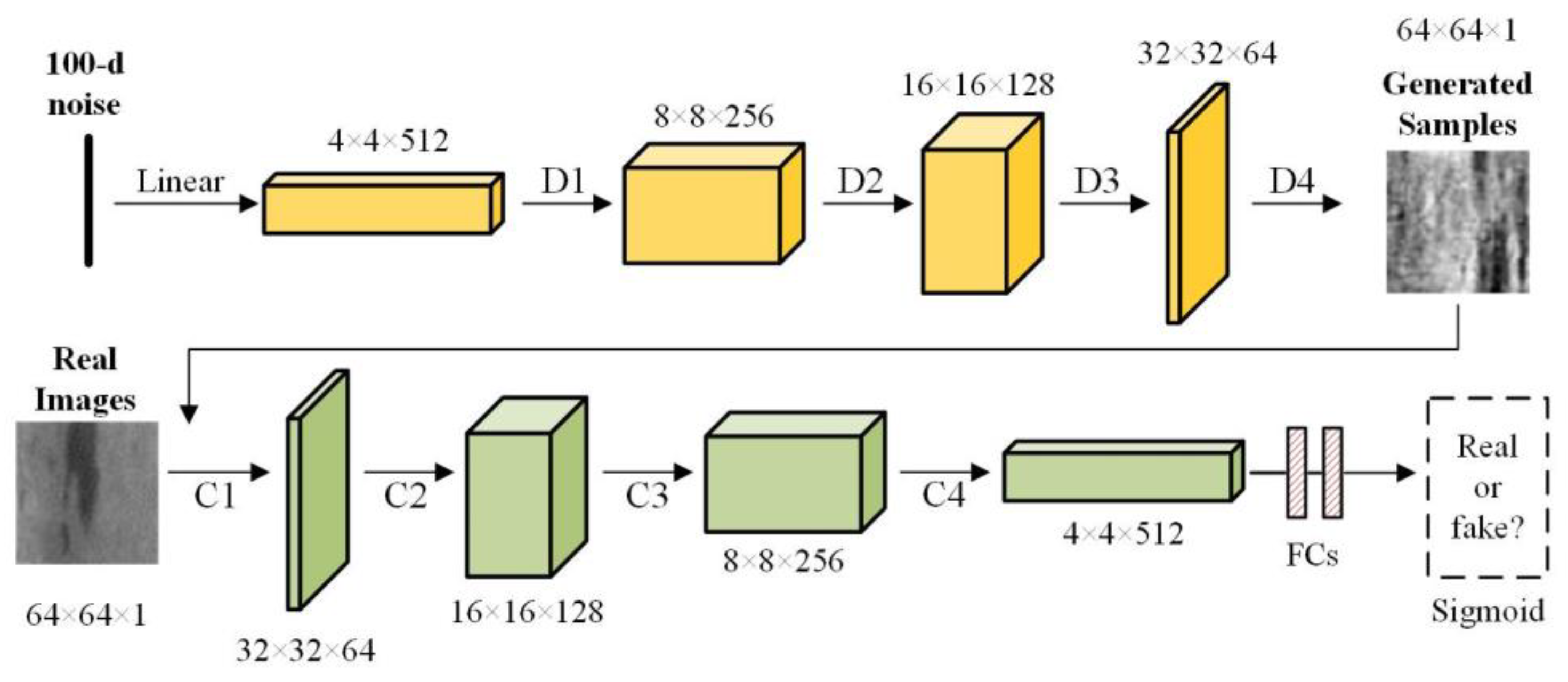
2.2. The Customized GAN

As already mentioned, the GAN has two sub-networks, a generator and a discriminator, which can be multi-layer perceptron [25], auto-encoders [29], or CNNs [30]. The customized GAN in our system uses CNNs as a backbone and is designed to be applicable to industrial gray images.

The GAN architecture is shown in Figure 1. For the generator, we feed into a 100 d random noise vector and reshape it to 4 × 4 × 8 using a linear function (because the mini-batch size is 64, the actual input size is 4 × 4 × 512 for each past). To enlarge the tensors, four deconvolutional layers are used with a kernel size of 5 × 5 and a stride of 2, denoted as {D1, D2, D3, D4}. Each deconvolutional layer follows a BN layer and a ReLU function, except the D4, which uses the tanh function. Finally, a sample that is 64 × 64 × 1 in size can then be generated. The discriminator receives the generated samples and real images as input. Similar to the generator, we use four convolutional layers to classify whether the input image is real or fake. These layers are also 5 × 5 in size with a stride of 2, denoted as {C1, C2, C3, C4}, each of which is equipped with a BN layer and a LeakyReLU function. The settings of output activation functions are followed by the outstanding conclusions in [27]. We add two fully connected layers to receive the last convolution feature maps and then feed them into a sigmoid output.

For all the datasets, we train the GAN on the same hyper-parameters. We use stochastic gradient descent (SGD) to train the models in the GAN with a mini-batch size of 64. All the weights are initialized from a normal distribution; the variance is 0 and the standard deviation is 0.02. The slope of leak is set to 0.2 in the LeakyReLU function. For each dataset, the GAN will be trained with a learning rate of 0.0001 for 600 epochs.

3. Methodology

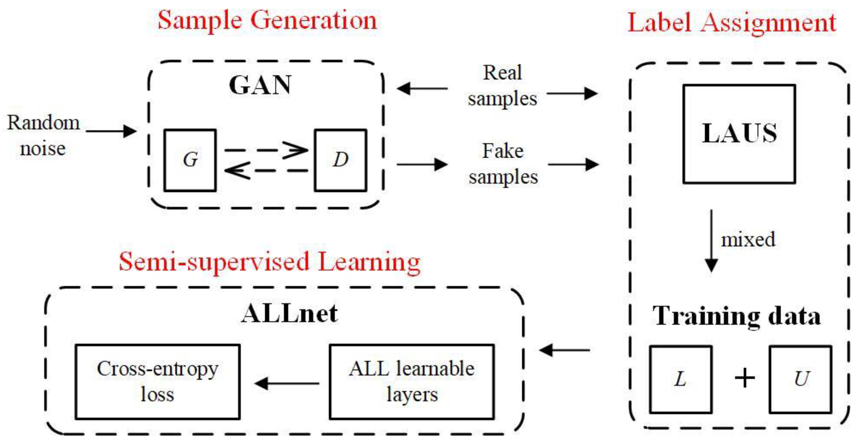
3.1. Overview of the SSL Framework

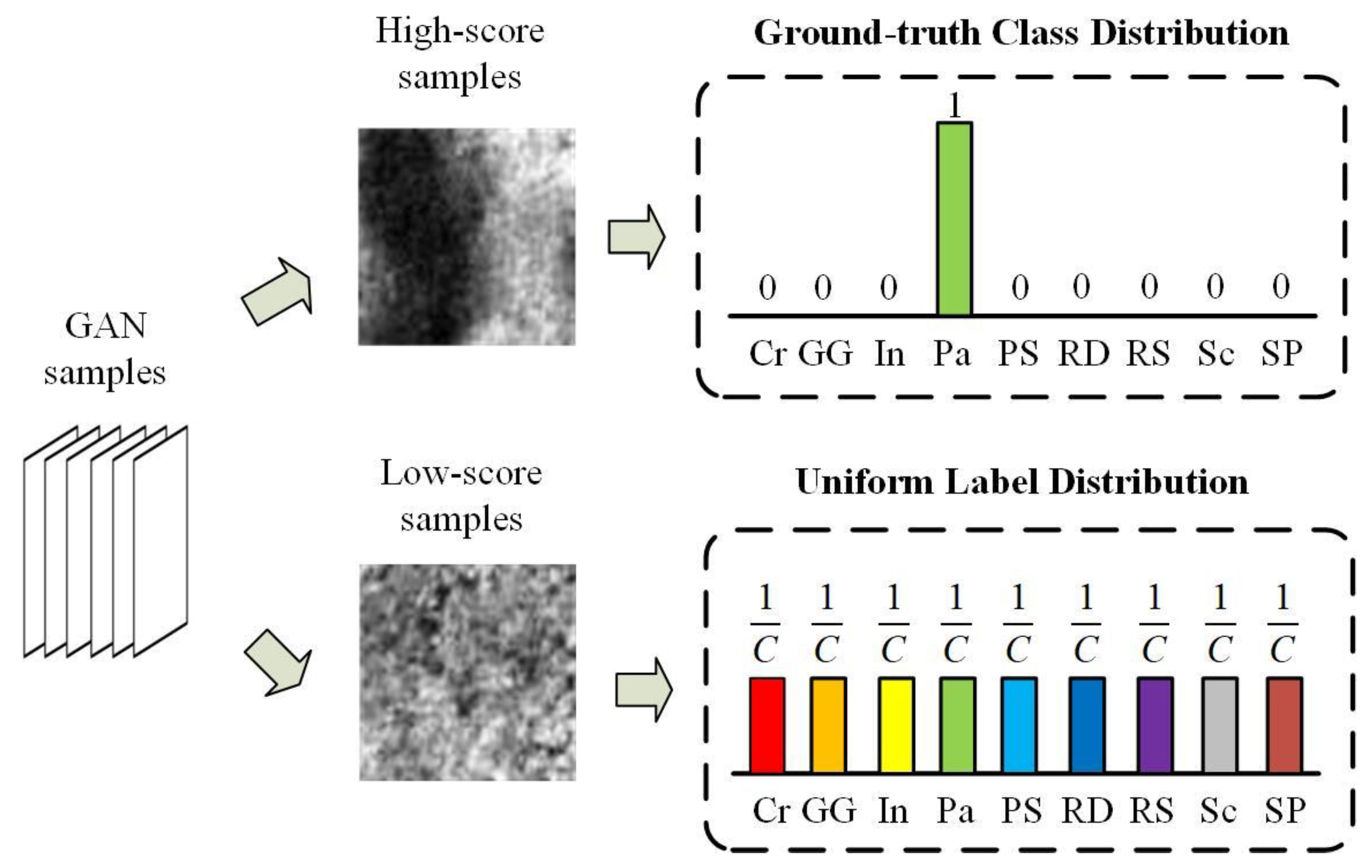
Figure 2 shows an overview of the proposed SSL framework, which consists of three parts: the customized GAN, the LAUS, and the ALLnet. In a single pass, the GAN receives labeled samples and noise as input and then generates unlabeled samples. Next, using the LAUS algorithm, it processes the generated samples in such a way that they can be included into labeled ones as training data. Finally, the ALLnet is trained on the mixed samples and thus has high defect classification ability.

3.2. LAUS Algorithm

In order to train with labeled samples, an SSL system makes a reasonable assumption on unlabeled samples and assigns them “labels”—often not the real labels. There are two assumptions that are commonly used for unlabeled samples. One is the “another label”, which creates an extra class label for the unlabeled samples [27]. The other is the “pseudo label”, which assigns each generated sample a ground-truth label according to the prediction output [28]. Both methods are effective, but their assumptions are too rough. For the unlabeled samples generated by GAN, “another label” considers that they have poor quality and places them into a new class outside existing ones, whereas “pseudo label” considers their quality as good as real samples and as belonging to the existing classes. In truth, however, the image quality produced by GAN is unpredictable, and the ratio of high-quality samples to low-quality samples in each category is also different.

Instead of creating a new class or pseudo labels, the proposed LAUS aims to isolate the whole GAN sample and assign them to different label distributions. Through the model that was trained on original samples, each GAN sample can obtain the corresponding class probability vector, the maximum of which will be treated as its class score. The high-score samples are assigned to their corresponding ground-truth class distributions. These samples join the existing classes, act as real data, and extend the labeled samples. The low-score samples are assigned to a uniform label distribution over all the existing classes. These samples, therefore, belong to neither the existing classes nor a new class (see Figure 3). After the LAUS process, the GAN samples that share common knowledge with the real samples can be included in training and not affect the learning direction towards unknown or fake classes. With this strategy, we can train powerful models on enough defect data and avoid the risk of over-fitting.

First of all, a CNN is supervised trained (i.e., the ALLnet in our pipeline) on real samples S_r, and the output feature maps can be written as:

$$z_j={\displaystyle \sum }_{i\in M_j}\sigma \left(w_i,b_i\right)$$

(2)

where w and b are the weights and bias of the i-th neuron in the j-th convolutional layer, and M_j is the set of input feature maps of the j-th convolutional layer. σ(∙) represents the activation function. After the training is completed, this model Ms is used to obtain the class score of the GAN sample. The output of the ALLnet is the softmax function that is defined as:

$${\theta }_j=\frac{e^{z_j}}{{\sum }_{k\in C}{e}^{z_k}}$$

(3)

For the GAN-generated samples (SGAN), the class score τ of each SGAN is the maximum prediction probability, τ = argmax (θ₁,…, θ_j), j∈C, where C is the number of ground-truth classes. According to τ, the SGAN are distributed into two sets of training data: labeled samples S_l and unlabeled samples S_u. The generated samples with high scores join S_l and receive the ground-truth class label “y”, corresponding to the maximum score. They are assigned the ground-truth class distribution q_GC as well as the S_r, and the q_GC can be written as:

$$q_{GC}=\left\{\begin{array}{c}0,k\ne y\\ 1, k=y\end{array}\right.$$

(4)

The rest of the generated samples are assigned the uniform label distribution q_UL that can be written as:

$$q_{UL}=\frac{1}{C}$$

(5)

Furthermore, if the real samples are so few that the start model M_s experiences serious over-fitting, the generated images would be regarded as unlabeled samples and assigned to the uniform label distribution. Finally, the LAUS transforms all the GAN samples into trainable data, and the details of it appear in Algorithm 1.

Algorithm 1: LAUS Algorithm
Input: GAN samples $S_{GAN}$, real samples $S_r$, and ground-truth class labels ${\theta }_{gt}$.
1:	Train ALLnet on {$S_{\mathrm{r}}$,${\theta }_{gt}$} => startup model $M_S$.
2:	for i in $S_{GAN}$:
3:	if no $M_S$:
4:	Label $S_{GAN}$ as a uniform label distribution ${\mathcal{L}}_{uniform}$.
5:	$S_u$←$S_{\mathrm{GAN}}$, $S_l$←$S_r$.
6:	break
7:	end if
8:	use $M_S$ on $S_{GAN}^{(i)}$=> class scores ${\tau }^{(i)}$.
9:	if ${\tau }^{(i)}\ge {\tau }_{threshold}$:
10:	label $S_{GAN}^{(i)}$ as ${\mathcal{L}}_{gt}$ according to ${\tau }^{(i)}$.
11:	$S_u$←$S_u+S_{GAN}^{(i)}$.
12:	else:
13:	label $S_{GAN}$ as ${\mathcal{L}}_{uniform}$.
14:	$S_l$←$S_l+S_{GAN}^{(i)}$..
15:	end if
16:	$S_l$←$S_r$.
17:	Training data $S_T$←$S_u+S_l$.
18:	end for
19:	Return  $S_T$

3.3. ALLnet

The baseline CNNs have become the common solution to deal with the representation learning on big data. These heavyweight networks, although they can achieve adequate results, may be unsuitable for some industrial scenes. For industrial inspection tasks, there are not many categories in one defect dataset in general, and therefore, we neither have enough defect data to train large networks nor need a network with so many neurons. In this context, we propose a novel network, ALLnet, as the representation learning machine of the semi-supervised pipeline. There are four blocks in ALLnet, denoted as {B1, B2, B3, B4}. Each block consists of three learnable layers: a 3 × 3 conv with a stride of 1, a 3 × 3 conv with a stride of 2, and a BN layer. We stack the layers with small 3 × 3 conv kernels, which can enhance the model capacity and complexity in fewer parameters [15]. The spatial pooling layer is replaced with stride convolution that lets the network learn how to down-sample, and the fully connected (fc) layers on top of convolutional features are replaced with a global average pooling (GAP) layer which has nearly zero parameters.

By the LAUS, we mixed the labeled and unlabeled samples into training data. Then, they are fed into the ALLnet for SSL until the maximum iteration is reached.

3.4. Training

3.4.1. Loss Function

In this paper, we use the cross-entropy loss for the SSL system. Let k∈{1, 2,..., C} be the predicted class, where C is the number of ground-truth classes. The cross-entropy loss can be formulated as:

$$L=-{\displaystyle \sum }_{k=1}^C\log (p\left(k\right))q\left(k\right)$$

(6)

where p(k) is the prediction probability that an input sample belongs to class k. It is derived from the softmax function, which normalizes the output of the previous fully connected layer. q(k) is the ground-truth class distribution. Let y be the corresponding ground-truth class, and q(k) can be defined as:

$$q\left(k\right)=\left\{\begin{array}{c}0\hspace{1em}k\ne y\\ 1\hspace{1em}k=y\end{array}\right.$$

(7)

Therefore, if we only consider the non-zero term, (6) can be equivalent to:

$$L=-\log (p\left(y\right))$$

(8)

As in Algorithm 1, the GAN samples have different assumptions. The high-score samples are assigned to ground-truth class distribution, whereas the low-score samples are assigned to a uniform label distribution q_LAUS(k), which is uniformed over the ground-truth classes. Let τ be the threshold of class score, and q_LAUS(k) can be defined as:

$$q_{LAUS}(k)=\left\{\begin{array}{c}q(k)\hspace{1em}p(k)\ge \tau \\ \frac{1}{C}\hspace{1em}p(k)<\tau \end{array}\right.$$

(9)

where the q(k) in the upper part is denoted in (7).

For the real images and the high-score samples, the cross-entropy loss is equivalent to (8), but for low-score samples, (6) can be equivalent to:

$$L=-\frac{1}{C}{\displaystyle \sum }_{k=1}^C\log (p\left(k)\right)$$

(10)

Combining (8), (10), and (6), the cross-entropy loss for our SSL framework can be rewritten as:

$$L=-\left(1-\omega \right)\log (p\left(y\right))-\alpha (n)\frac{\omega }{C}{\displaystyle \sum }_{k=1}^C\log (p\left(k)\right)$$

(11)

If the input image is labeled, ω = 0. If the input image is unlabeled, ω = 1. Since there are more labeled samples than unlabeled ones in training data, a penalty function α(n) is incorporated into the unlabeled item, which can avoid making the learning tend to rapid deterioration when too many GAN samples are added. α(n) can be written as:

$$\alpha (n)=\left\{\begin{array}{c}0\hspace{1em}\hspace{1em}n<N_1\\ \frac{n-N_1}{N_2-N_1}{\alpha }_t\hspace{1em}{N}_1\le n<N_2\\ {\alpha }_t\hspace{1em}\hspace{1em}{N}_2\le n \end{array}\right.$$

(12)

where n is the number of generated samples and αt is the threshold, which is set to 0.8 in this paper. For SSL, the number of unsupervised samples should not be less than that of the supervised ones. Let N_real be the number of real training images, N₁ is equal to N_real, and N₂ is five times the value of N_real.

3.4.2. Implementation

We train the SSL model to minimize the loss function in (11). All the input images, consisting of real and GAN ones, are resized as 64 × 64 × 1 and randomly mixed in training data. The mini-batch size of each input is 128. We train the models with the Adam optimizer [31] with the exponential decay parameters β₁ and β₂ set to 0.9 and 0.99, respectively. We train the model with a learning rate of 0.0001 for 100,000 mini-batch iterations. All the experiments were run in Python with Tensorflow packages on an Intel Core i7, 3.3 GHz with 64-GB RAM and a NVIDIA TITAN Xp GPU workstation.

4. Experiments

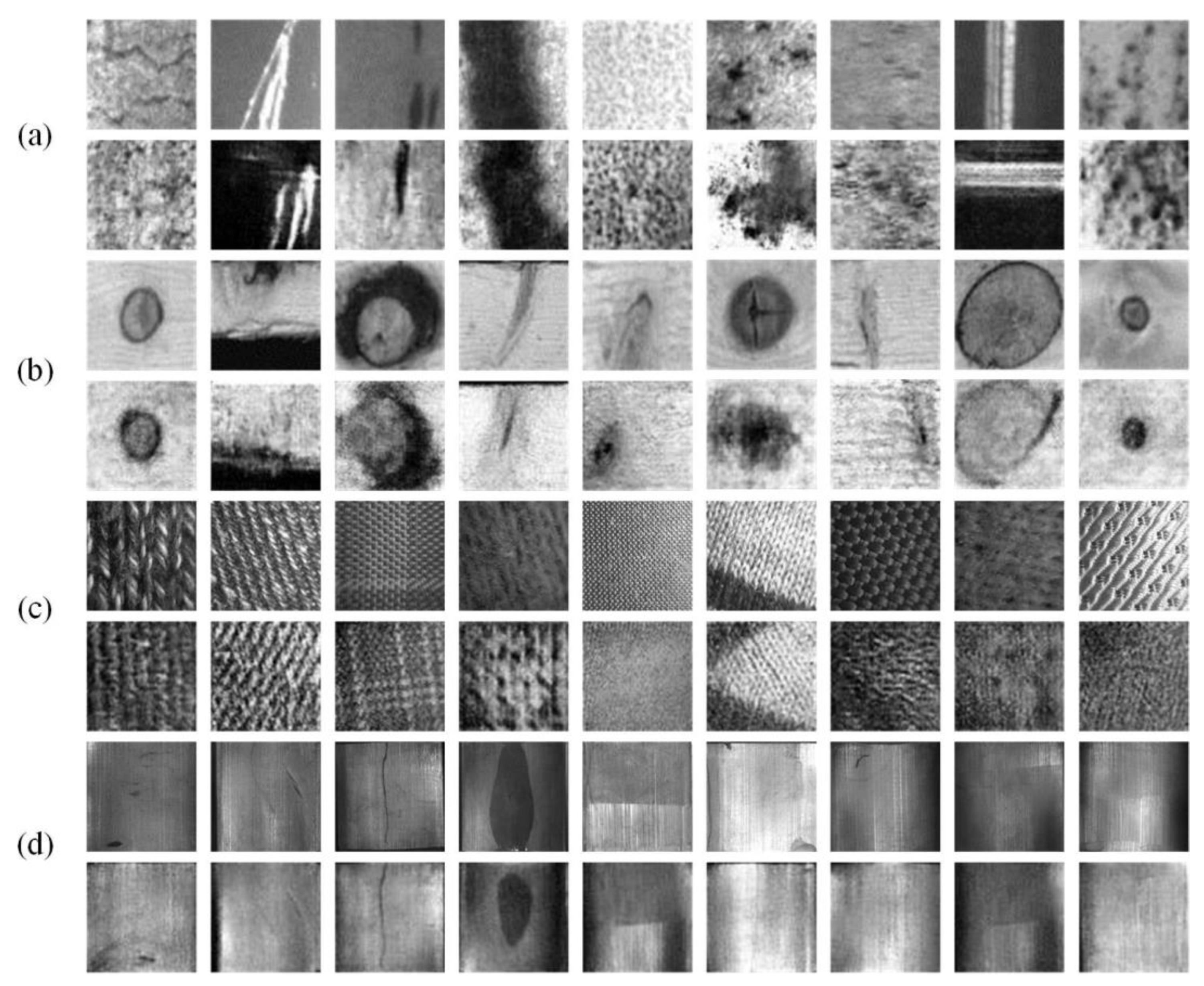
4.1. Defect Datasets

The proposed method is evaluated on four types of defect datasets, namely the wood defect dataset KNOTS [2], the textile dataset Fabrics [3], the steel plate defect dataset NEU-CLS-64 [32], and the magnetic tile defect dataset MT [33]. NEU-CLS-64 is improved on the defect dataset NEU-CLS, which contains 1800 images of six defect classes. The motive to recreate the NEU-CLS-64 is that multiple and even unknown defects exist in an image. So, we extended the NEU-CLS in terms of quantity and category. In more detail, every image was resized to 192 × 192 and center-cropped into nine 64 × 64 images. Then, we discarded the following cropped images: the ones with heavily occluded defects, edge-truncated defects, and no defect. Finally, the updated dataset NEU-CLS-64 assembles approximately 7000 tiny images with nine defect classes, i.e., crazing (Cr), grooves and gouges (GG), inclusion (In), patches (Pa), pitted surface (PS), rolling dust (RD), rolled-in scale (RS), scratches (Sc), and spots (Sp). The details of the NEU-CLS-64 and three other defect datasets are summarized in

Table 1. Details of four defect datasets.

Datasets (Num.)	Defect Type and Num.
NEU-CLS-64 (7226)	Cr (1210), GG (296), In (775), Pa (1148), PS (797), RD (200), RS (1589), Sc (773), SP (438).
KNOTS (425)	Dry (69), Edge (65), Encased (30), Horn (35), Leaf (47), Sound (179).
Fabrics (1173)	Cotton (588), Denim (162), Nylon (57), Polyester (226), Silk (50), Wool (90).
MT (392)	Blowhole (115), Break (85), Crack (57), Fray (32), Uneven (103).

, and the examples of each dataset are shown in Figure 4. In this section, we mainly report results on the NEU-CLS-64, which is a relatively large-scale dataset; the other three datasets serve as auxiliary datasets for further verification. All the datasets use the same train/test ratio in experiments, and the ratio is 7:3 in this study.

4.2. GAN Results

We first need to ensure that most samples generated by GAN are available. The examples of GAN samples are shown in Figure 4. For most types of defects, GAN samples cannot be intuitively distinguished from real images by human eyes. However, several images of some defect categories are fuzzy, such as the “crazing” in the NEU-CLS-64 (see the first column in Figure 4a). Next, we want to prove that the unlabeled GAN samples can boost the classification performance. Since unlabeled samples are relatively easy to obtain, we hope that these generated samples have similar semantic information to the real samples, and thereby can assist or replace the labeled samples that are too difficult to collect. In order to verify this, we added different numbers of GAN samples generated on the NEU-CLS-64 into training, and the results are given in

Table 2. Comparing LAUS with related algorithms.

${\mathit{S}}_{\mathit{G}\mathit{A}\mathit{N}}:{\mathit{S}}_{\mathit{r}\mathit{e}\mathit{a}\mathit{l}}$	LAUS	Another Label	Pseudo Label
	acc. (%)	acc. (%)	acc. (%)
0 (baseline)	96.24	96.24	96.24
1×	98.04	98.19	98.39
2×	98.40	98.60	98.55
3×	99.37	98.92	98.41
4×	99.13	99.04	97.90
5×	98.97	99.02	97.61

. From this table, we can safely conclude that the unlabeled GAN samples can share common knowledge with the labeled ones, and by the addition of GAN samples, there is a significant increase in classification accuracy. As we discussed in Section 3, LAUS makes a more reasonable assumption for GAN samples and therefore achieves the best results. The classification accuracy is improved by approximately three points when 1 × GAN samples are added compared to the original samples. As the number of GAN samples increases, classification accuracy increases gradually, and it reaches the peak when 3 × GAN samples are added. Since the low-score samples are much more abundant than the high-score ones, the accuracy would tend to deteriorate if too many GAN samples are added, but even so, adding 5×GAN samples still gives a 3.73% improvement in accuracy over the baseline.

We evaluated the GAN samples for each category of the NEU-CLS-64 in detail, and the results are shown in Figure 5. We wanted to explore how unlabeled samples contribute to overall accuracy when they are trained along with labeled samples. From Figure 5, we observe that the addition of GAN samples can lead to a consistent decrease in error rate for all the defect classes. Unsurprisingly, the ratio of high-score and low-score samples produced on each class is quite different. The class with a higher error rate seems to produce fewer high-score samples, but enough low-score samples can still reduce the error rate. Like the Cr, although it only has only 2% high-score samples of the GAN samples, the Top-1 error rate of Cr dropped dramatically by approximately 5%.

4.3. Comparison with Other Label Assignment Algorithms

We compare the LAUS with the “another label” and “pseudo label”, which can also be used in the semi-supervised framework. The experimental results on the NEU-CLS-64 are also listed in Table 2. In this table, we observe that both methods are effective and the LAUS can also exceed them by 1~2 points when they all reach the peak. We consider the reason for this is that LAUS’s assumption for GAN samples is more reasonable. The “another label” makes a coarse assumption for the GAN samples that are all considered as low-score ones. So, as the number of GAN samples increases, the accuracy rises gradually. The “pseudo label” gives an over-optimistic evaluation of the GAN samples and puts them all in the ground-truth classes. It causes the accuracy to peak before many GAN samples are added, and then drops sharply due to too many low-score samples making the learning process deteriorate. Unlike the onefold assumptions of the “another label” and “pseudo label”, the LAUS performs different assignments for the GAN samples, which may be the reason why the LAUS has a superior performance.

4.4. Comparison with Baseline CNNs

We replace the ALLnet with other baseline CNNs to evaluate its effect in a semi-supervised framework. Since baseline CNNs require a great amount of training data, we enlarged the training set for a fair comparison, where 3 × GAN samples are added. The input size and weight parameters of CNNs used in experiments are different, and hence we use different training epochs and minibatch sizes for them. The time of a float operation is used as the measure of runtime. The AlexNet and VGG16 are trained with a minibatch size of 64 for 300 epochs, and the InceptionV3 and ResNet101 with a minibatch size of 32 for 600 epochs. The training configuration for ALLnet is defined in Section 3. The results on NEU-CLS-64 are listed in

Table 3. Comparison with baseline CNNs.

Models	Input Size	Parameters	Accuracy (%)	Runtime (ms/Float)
AlexNet	224 × 224	5.8×107	99.10	42.1
VGG16	224 × 224	13×107	99.62	66.2
InceptionV3	299 × 299	2.4×107	99.29	21.0
ResNet101	224 × 224	4.0×107	99.47	29.7
ALLnet(2B)	64 × 64	0.2×106	97.50	6.9
ALLnet(3B)	64 × 64	0.7×106	98.44	8.4
ALLnet(4B) *	64 × 64	2.9×106	99.37	8.6
ALLnet(4B)	128 × 128	2.9×106	99.37	21.0
ALLnet(5B)	64 × 64	12×106	99.38	10.2

* represents that this model is used in our semi-supervised framework. “B” indicates the block of the ALLnet, which consists of two conv layers and a BN layer.

. It is no surprise that the strong baseline CNNs obtained adequate results—the accuracy exceeds 99%. However, a large input size requires enough memory and redundant parameters and has excessive computation costs, which can slow down the convergence and increase the computation time. By comparison, the ALLnet not only achieved the same level of accuracy as the large networks, but also has a simpler structure and less computing time. Furthermore, we also make a detailed assessment of the internal structure of the ALLnet, mainly to judge the impact of the number of blocks and input size on the model. We observe that each additional block in the ALLnet brings an approximately 1% increase in the overall accuracy, and this trend will continue until there are four blocks in the model. Another finding is that expanding input size can hardly increase accuracy but can greatly reduce computational speed. According to the above results, we can conclude that the ALLnet with four blocks achieved the best trade-off between speed and precision, and a large network seems to be unnecessary for industrial inspection tasks.

4.5. Comparison with Other Defect Classifiers

We compare our SSL method with state-of-the-art defect classifiers based on supervised learning or transfer learning. The methods selected for comparison include the supervised ones by Zhou et al. [12] and Hossain et al. [13], and the transfer learning-based ones are Decaf [14] and MVM-VGG [16]. For simplicity, we call these four methods S1, S2, T1, and T2, respectively. These methods are reproduced by Tensorflow as our method for fair comparison. The contrast experiments were carried out on the four aforementioned defect datasets by adding different numbers of GAN samples. These GAN samples were added in two ways: one is to compensate the difference between classes to restore a dataset into a balanced one (balance mode, “B” for short); the other is to follow the original inter-class ratio (unbalance mode, “U” for short). The results are shown in

Table 4. Comparison with other defect classifiers on four defect datasets.

Dataset		NEU-CLS-64					KNOTS
Methods		S1	S2	T1	T2	Ours	S1	S2	T1	T2	Ours
0 (baseline)		87.50	88.14	92.87	97.00	96.24	79.69	73.44	80.21	73.81	80.38
1 × GANs	B	93.25	92.04	96.84	97.87	98.04	84.38	89.06	85.28	89.31	89.06
	U	93.64	91.16	95.66	96.87	97.86	78.91	84.38	82.09	85.29	86.72
2 × GANs	B	95.62	95.40	97.76	98.58	98.40	90.63	89.84	88.69	92.30	91.14
	U	94.72	93.25	95.89	98.00	98.79	87.50	85.90	83.56	88.69	90.63
3 × GANs	B	97.94	97.11	99.10	99.34	99.37	94.53	94.01	96.62	97.49	97.49
	U	96.63	95.16	97.60	98.89	98.87	93.49	91.41	92.20	94.62	95.31
4 × GANs	B	97.26	95.81	98.55	99.12	99.13	92.97	92.96	93.02	97.00	95.00
	U	96.13	94.28	96.16	92.87	98.36	88.80	90.89	90.55	92.37	94.53
5 × GANs	B	96.65	95.66	97.75	98.13	98.87	91.41	93.49	92.37	96.53	94.68
	U	84.90	-	91.34	90.43	84.91	88.67	91.46	86.32	93.02	83.33
Datasets		Fabrics					MT
0 (baseline)		-	-	73.47	82.33	65.42	96.88	90.31	92.60	59.32	92.19
1 × GANs	B	67.71	73.70	83.33	90.55	80.02	91.41	92.19	94.88	66.87	96.09
	U	69.27	-	79.93	88.22	77.60	89.84	91.41	92.90	64.62	95.31
2 × GANs	B	86.91	85.32	90.10	91.70	88.93	92.58	-	97.51	79.62	97.40
	U	79.84	82.34	86.40	91.09	84.21	94.53	96.88	92.33	64.99	92.19
3 × GANs	B	90.94	91.99	91.90	93.07	93.80	95.31	-	99.09	82.84	99.22
	U	90.00	90.04	89.01	92.80	90.31	99.22	98.18	96.68	81.63	97.65
4 × GANs	B	87.30	89.55	91.04	91.61	91.40	97.92	-	98.82	82.77	98.17
	U	88.09	86.33	88.64	91.54	90.09	97.66	97.66	95.31	82.59	97.39
5 × GANs	B	85.68	89.50	87.99	92.98	90.04	96.61	-	97.79	83.82	98.88
	U	83.33	82.50	87.50	91.15	86.98	97.40	97.27	95.01	85.77	94.27

.

In the four defect datasets, our method achieves 3.13%, 17.11%, 28.38%, and 7.03% improvements in accuracy compared to the baseline, respectively. Meanwhile, our method at the point of 3 × GANs consistently obtained the best results and is superior to other methods for each dataset. For each dataset, our method can work well even if the original data are limited, which also shows that our method performs better than other methods in terms of generalization and robustness. Moreover, our method can easily correct the original unbalanced defect dataset into a balanced one, which brings an improvement in accuracy.

5. Conclusions

In this paper, we propose a semi-supervised learning method that mainly deals with data-limited defect classification tasks. This method has no need for extra collection of defect data but uses a customized GAN to generate samples. Through the proposed LAUS, the GAN samples can be trained with the limited original samples simultaneously. We also designed the ALLnet, which is trained on these samples in a semi-supervised manner. Extensive experiments on four different defect datasets have shown that under the semi-supervised learning framework, we obtained substantial accuracy improvements that range from 3.13% to 28.38%. Our method can be more precise and robust than the previous state-of-the-art transfer learning and supervised learning methods, and is effective for defect classification when the original samples are limited.

References

1. Yu, H.; Li, Q.; Tan, Y.; Gan, J.; Wang, J.; Geng, Y.-A.; Jia, L. A Coarse-to-Fine Model for Rail Surface Defect Detection. IEEE Trans. Instrum. Meas. 2018, 68, 656–666. [Google Scholar] [CrossRef]
2. Niskanen, M.; Kauppinen, H. Wood inspection with non-supervised clustering. Mach. Vis. Appl. 2003, 13, 275–285. [Google Scholar] [CrossRef] [Green Version]
3. Kampouris, C.; Zafeiriou, S.; Ghosh, A.; Malassiotis, S. Fine-grained material classification using micro-geometry and reflectance. In Proceedings of the European Conference on Computer Vision (ECCV), Amsterdam, The Netherlands, 8–12 October 2016; pp. 778–792. [Google Scholar]
4. Kahraman, Y.; Durmuşoğlu, A. Deep learning-based fabric defect detection: A review. Text. Res. J. 2022. [Google Scholar] [CrossRef]
5. Kahraman, Y.; Durmuşoğlu, A. Classification of Defective Fabrics Using Capsule Networks. Appl. Sci. 2022, 12, 5285. [Google Scholar] [CrossRef]
6. Zhang, Z.; Wen, G.; Chen, S. Audible Sound-Based Intelligent Evaluation for Aluminum Alloy in Robotic Pulsed GTAW Mechanism, Feature Selection, and Defect Detection. IEEE Trans Ind. Inf. 2018, 14, 2973–2983. [Google Scholar] [CrossRef]
7. Park, Y.; Kweon, I.S. Ambiguous Surface Defect Image Classification of AMOLED Displays in Smartphones. IEEE Trans. Ind. Inform. 2016, 12, 597–607. [Google Scholar] [CrossRef]
8. Wang, H.Y.; Zhang, J.; Tian, Y.; Chen, H.Y.; Sun, H.X.; Liu, K. A Simple Guidance Template-Based Defect Detection Method for Strip Steel Surfaces. IEEE Trans. Ind. Inform. 2018, 15, 2798–2809. [Google Scholar] [CrossRef]
9. Luo, Q.; Sun, Y.; Li, P.; Sun, Y.; Li, P.; Simpson, O.; Tian, L.; He, Y. Generalized Completed Local Binary Patterns for Time-Efficient Steel Surface Defect Classi-fication. IEEE Instrum. Meas 2018, 68, 667–679. [Google Scholar] [CrossRef] [Green Version]
10. Zhou, S.; Chen, Y.; Zhang, D.; Xie, J.; Zhou, Y. Classification of surface defects on steel sheet using convolutional neural networks. Mater. Teh. 2017, 51, 123–131. [Google Scholar] [CrossRef]
11. Hossain, M.S.; Al-Hammadi, M.; Muhammad, G. Automatic Fruit Classification Using Deep Learning for Industrial Ap-plications. IEEE Trans. Ind. Inf. 2019, 15, 1027–1034. [Google Scholar] [CrossRef]
12. Huang, H.-W.; Li, Q.-T.; Zhang, D.-M. Deep learning based image recognition for crack and leakage defects of metro shield tunnel. Tunn. Undergr. Space Technol. 2018, 77, 166–176. [Google Scholar] [CrossRef]
13. Wen, W.; Xia, A. Verifying edges for visual inspection purposes. Pattern Recognit. Lett. 1999, 20, 315–328. [Google Scholar] [CrossRef]
14. Krizhevsky, A.; Sutskever, I.; Hinton, G.E. ImageNet classification with deep convolutional neural networks. In Proceedings of the ProceNeural Information Processing Systems (NIPS), Lake Tahoe, NV, USA, 3–6 December 2012; pp. 1097–1105. [Google Scholar]
15. Simonyan, K.; Zisserman, A. Very deep convolutional networks for large-scale image recognition. In Proceedings of the International Conference on Learning Representations (ICLR), San Diego, CA, USA, 7–9 May 2015. [Google Scholar]
16. Szegedy, C.; Vanhoucke, V.; Ioffe, S.; Shlens, J.; Wojna, Z. Rethinking the Inception Architecture for Computer Vision. In Proceedings of the IEEE Conference on Computer Vision and Pattern Recognition (CVPR), Las Vegas, NV, USA, 27–30 June 2016; pp. 2818–2826. [Google Scholar] [CrossRef] [Green Version]
17. He, K.; Zhang, X.; Ren, S.; Sun, J. Deep residual learning for image recognition. In Proceedings of the 2016 IEEE Conference on Computer Vision and Pattern Recognition (CVPR), Las Vegas, NV, USA, 27–30 June 2016; pp. 770–778. [Google Scholar] [CrossRef] [Green Version]
18. Ren, R.; Hung, T.; Tan, K.C. A Generic Deep-Learning-Based Approach for Automated Surface Inspection. IEEE Trans. Cybern. 2017, 48, 929–940. [Google Scholar] [CrossRef] [PubMed]
19. Yang, H.; Mei, S.; Song, K.; Tao, B.; Yin, Z. Transfer-Learning-Based Online Mura Defect Classification. IEEE Trans. Semicond. Manuf. 2017, 31, 116–123. [Google Scholar] [CrossRef]
20. Natarajan, V.; Hung, T.-Y.; Vaikundam, S.; Chia, L.-T. Convolutional networks for voting-based anomaly classification in metal surface inspection. In Proceedings of the IEEE International Conference on Industrial Technology (ICIT), Toronto, ON, Canada, 22–25 March 2017; pp. 986–991. [Google Scholar] [CrossRef]
21. Lecun, Y.; Bengio, Y.; Hinton, G. Deep learning. Nature 2015, 521, 436–444. [Google Scholar] [CrossRef]
22. Liu, C.; Su, K.; Yang, L.; Li, J.; Guo, J. Detection of Complex Features of Car Body-in-White under Limited Number of Samples Using Self-Supervised Learning. Coatings 2022, 12, 614. [Google Scholar] [CrossRef]
23. Papandreou, G.; Chen, L.-C.; Murphy, K.P.; Yuille, A.L. Weakly-and semi-supervised learning of a deep convolutional network for semantic image segmentation. In Proceedings of the International Conference on Computer Vision. (ICCV), Santiago, Chile, 13–16 December 2015; pp. 1742–1750. [Google Scholar]
24. Song, K.; Wang, J.; Bao, Y.; Huang, L.; Yan, Y. A Novel Visible-Depth-Thermal Image Dataset of Salient Object Detection for Robotic Visual Perception. IEEE/ASME Trans. Mechatron. 2022, 1–12. [Google Scholar] [CrossRef]
25. Wu, H.; Prasad, S. Semi-Supervised Deep Learning Using Pseudo Labels for Hyperspectral Image Classification. IEEE Trans. Image Process 2017, 27, 1259–1270. [Google Scholar] [CrossRef]
26. Odena, A. Semi-Supervised Learning with Generative Adversarial Networks. In Proceedings of the International Conference on Machine Learning. (ICML), New York, NY, USA, 6–11 June 2015. [Google Scholar]
27. He, D.; Xu, K.; Zhou, P.; Dongdong, Z. Surface defect classification of steels with a new semi-supervised learning method. Opt. Lasers Eng. 2019, 117, 40–48. [Google Scholar]
28. Larsen, A.B.L.; Kaae, S.S.; Winther, O. Autoencoding beyond pixels using a learned similarity metric. In Proceedings of the International Conference on Machine Learning. (ICML), New York, NY, USA, 19–24 June 2016; pp. 1558–1566. [Google Scholar]
29. Alec, R.; Luke, M.; Soumith, C. Unsupervised representation learning with deep convolutional generative adversarial networks. arXiv 2015, arXiv:1511.06434. [Google Scholar]
30. Li, P.; Chen, Z.; Yang, L.T.; Zhang, Q.; Deen, M.J. Deep Convolutional Computation Model for Feature Learning on Big Data in Internet of Things. IEEE Trans. Ind. Inform. 2017, 14, 790–798. [Google Scholar] [CrossRef]
31. Kingma, P.D.; Ba, J. Adam: A Method for Stochastic Optimization. In Proceedings of the International Conference on Learning Representations (ICLR), San Diego, CA, USA, 7–9 May 2015. [Google Scholar]
32. Song, K.; Yan, Y. A noise robust method based on completed local binary patterns for hot-rolled steel strip surface defects. Appl. Surf. Sci. 2013, 285, 858–864. [Google Scholar] [CrossRef]
33. Huang, Y.; Qiu, C.; Guo, Y. Saliency of magnetic tile surface defects. In Proceedings of the 14th IEEE International Conference on Auto-Mation and Engineering, Munich, Germany, 18–22 June 2018. [Google Scholar]
Figure 1. The architecture of the customized GAN.
Coatings 12 01707 g001
Figure 2. The proposed SSL framework. “L” and “U” represent labeled samples and unlabeled samples.
Coatings 12 01707 g002
Figure 3. The label distributions for different generated samples.
Coatings 12 01707 g003
Figure 4. Examples of the real images and the GAN samples of the four defect datasets. In each group, the top row shows real images and the bottom row shows GAN samples. (a) NEU-CLS-64, (b) KNOTS, (c) Fabrics, (d) MT.
Coatings 12 01707 g004
Figure 5. The effects of adding GAN samples on each defect class of NEU-CLS-64. (a) The Top-1 error rate comparison between no GAN samples added (baseline) and adding 3 × GAN samples. (b) The percentage of high-score samples and low-score samples of each defect class in the 3 × GAN samples.
Coatings 12 01707 g005aCoatings 12 01707 g005b