Nucleic Acid Quantification by Multi-Frequency Impedance Cytometry and Machine Learning

 and
and
Abstract
:
1. Introduction
2. Materials and Methods
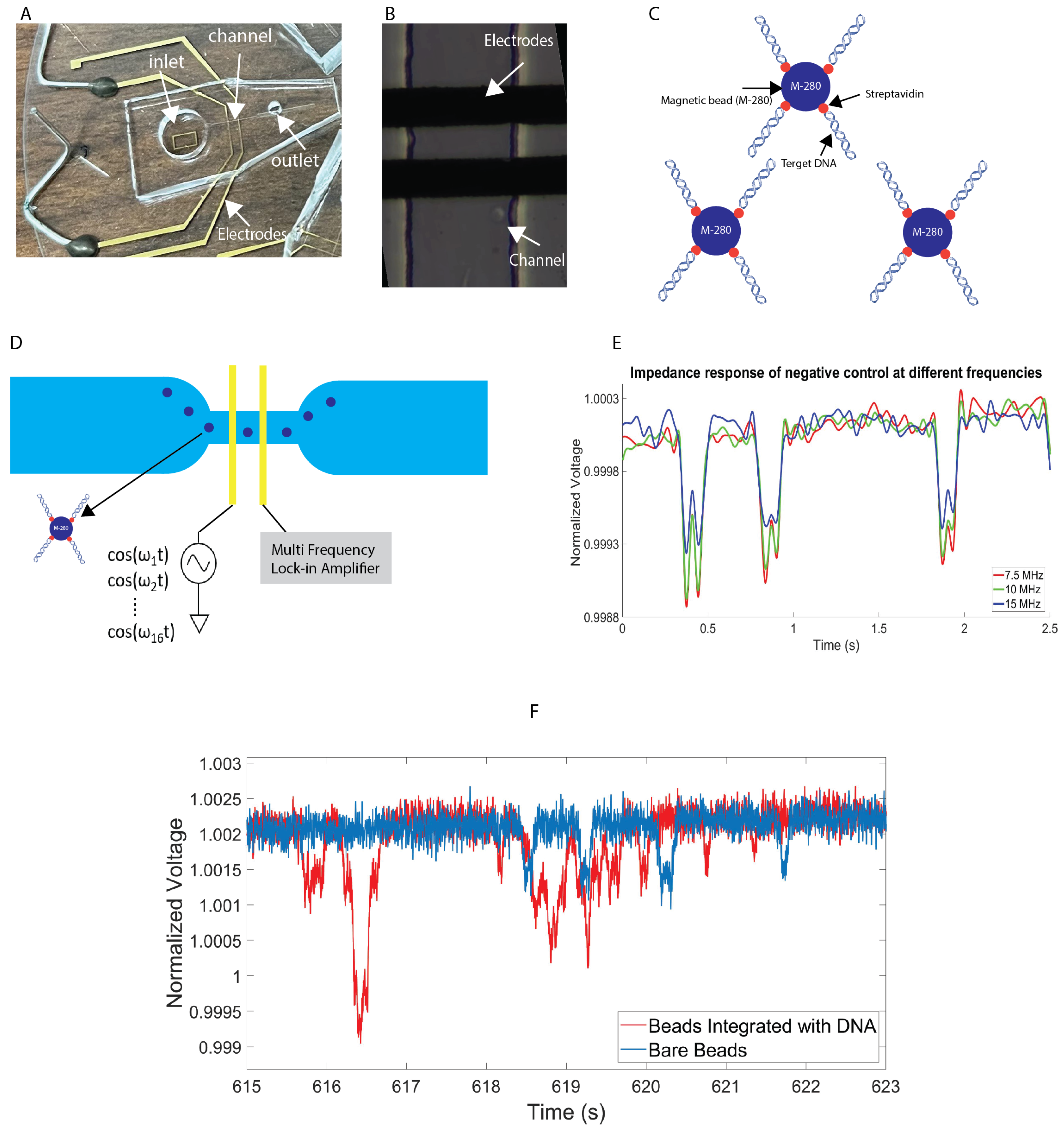
2.1. Experimental Setup
- Biotinylated oligos was synthesized by IDT (Coralville, IA, USA), which is used to amplify different fragment sizes of DNA; in this case the fragment size is 300 bp.
- The PCR product was purified by using a Qiaquick PCR purification kit to remove any unincorporated biotinylated oligos.
- The PCR was eluted in water and quantified for immobilization to the streptavidin coated on 2.8 μm (M280) beads.
- The purified biotinylated DNA was immobilized with beads in room temperature for 15 min using gentle rotation at 2000 rpm.
- The biotinylated DNA-coated beads were separated on a magnet and washed subsequently.
2.2. Dataset
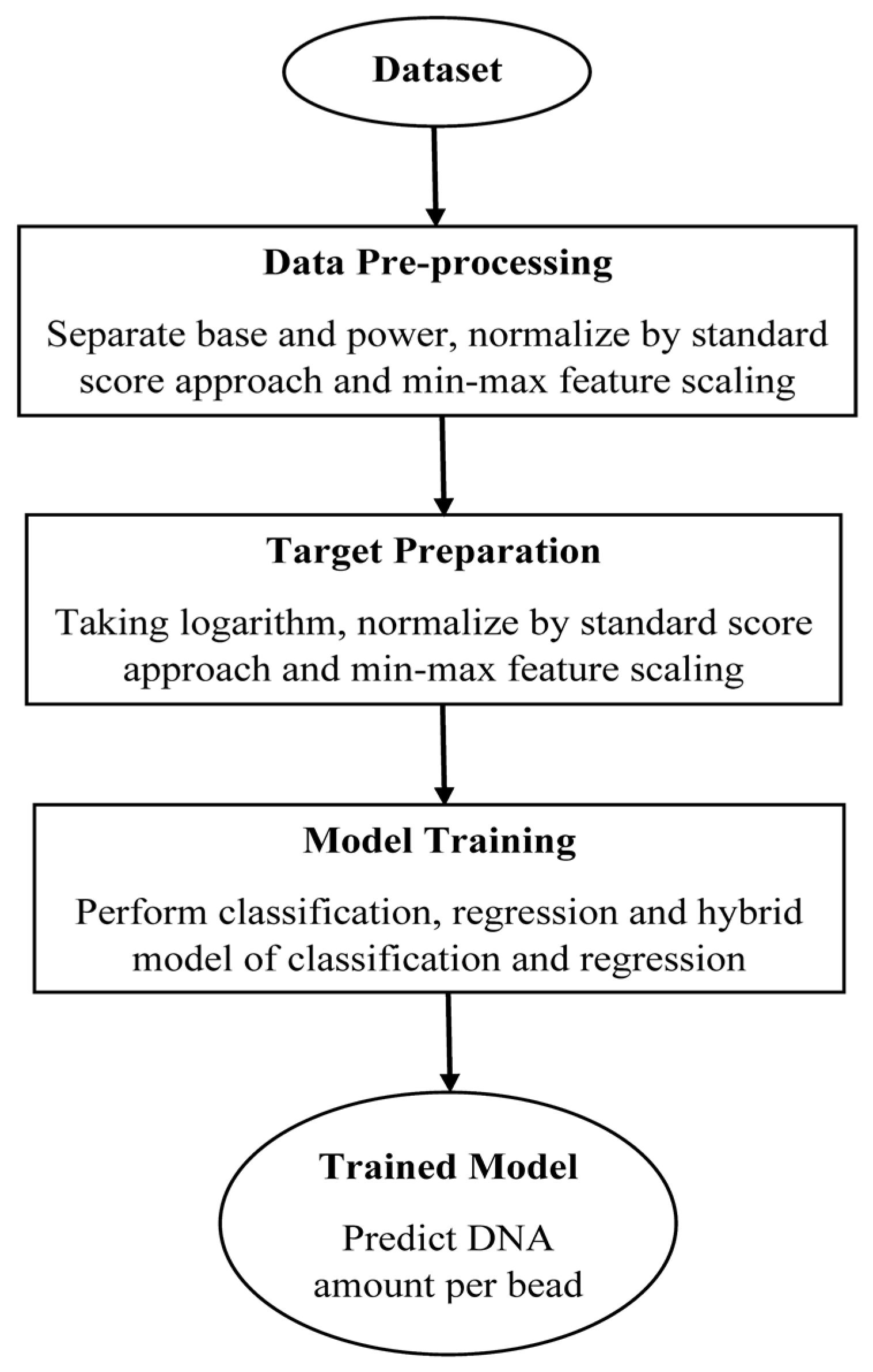
2.3. Data Preprocessing
2.4. Target Preparation
2.5. Model Training
3. Results
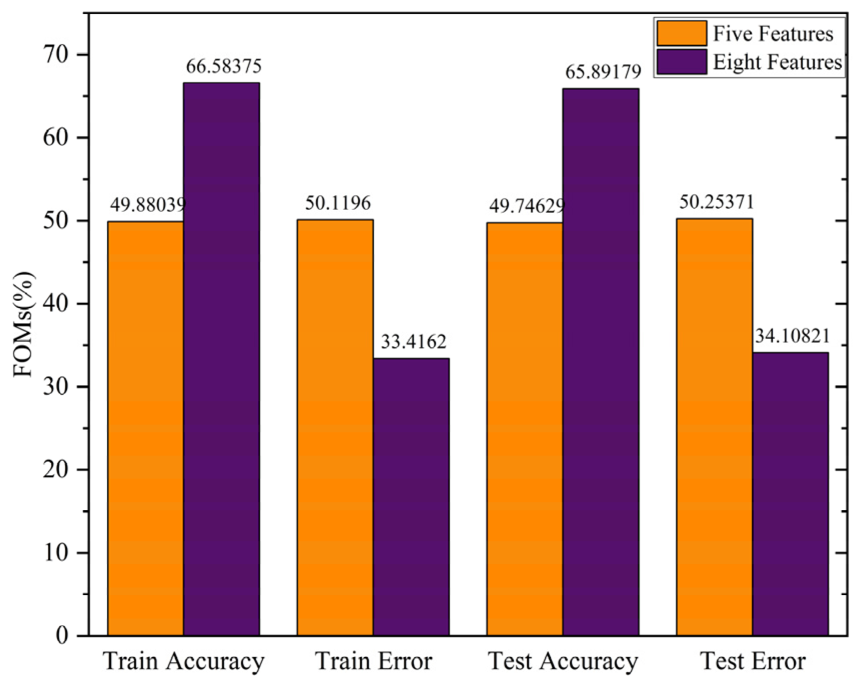
3.1. Feature Selection
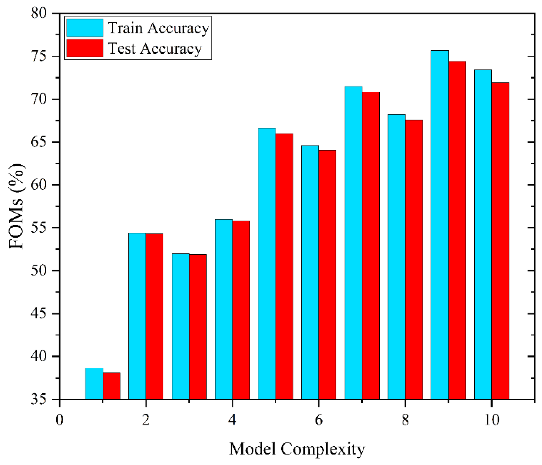
3.2. Classification
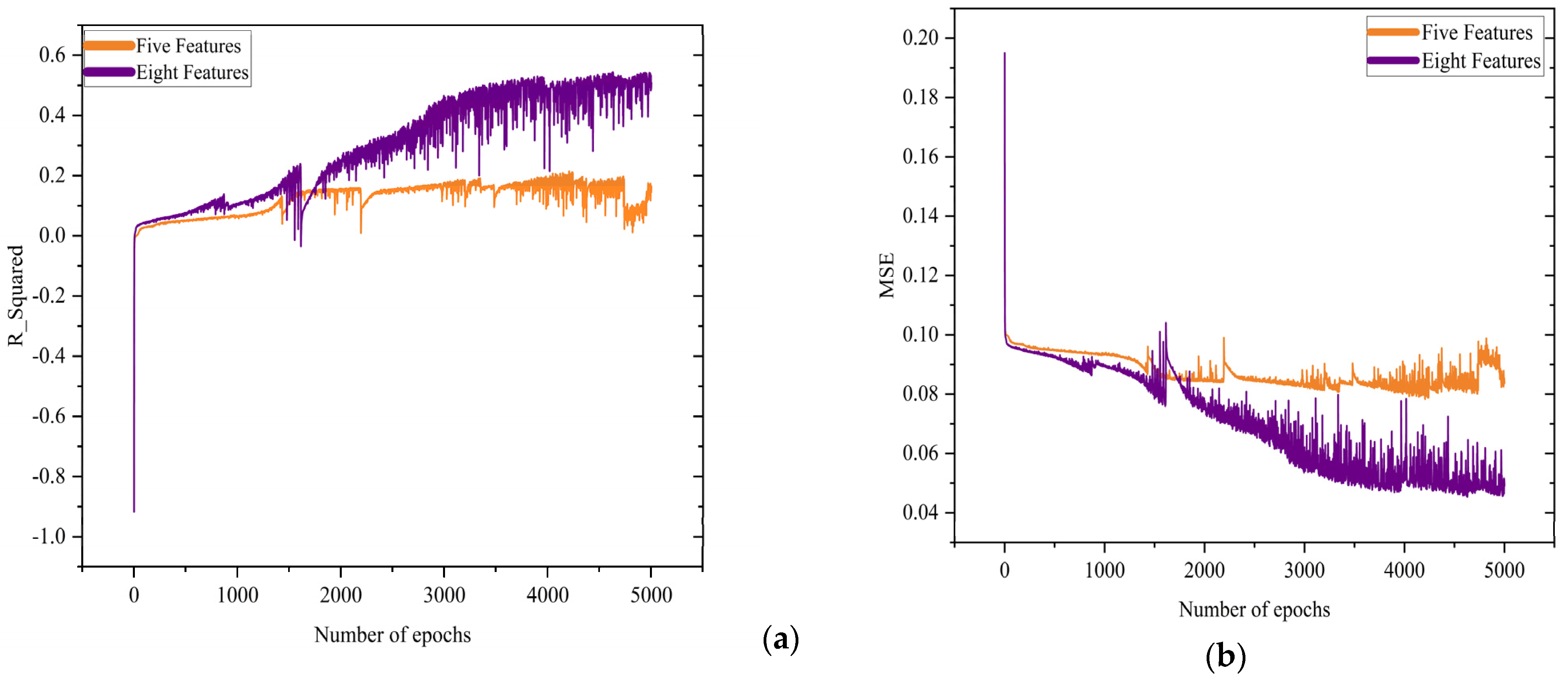
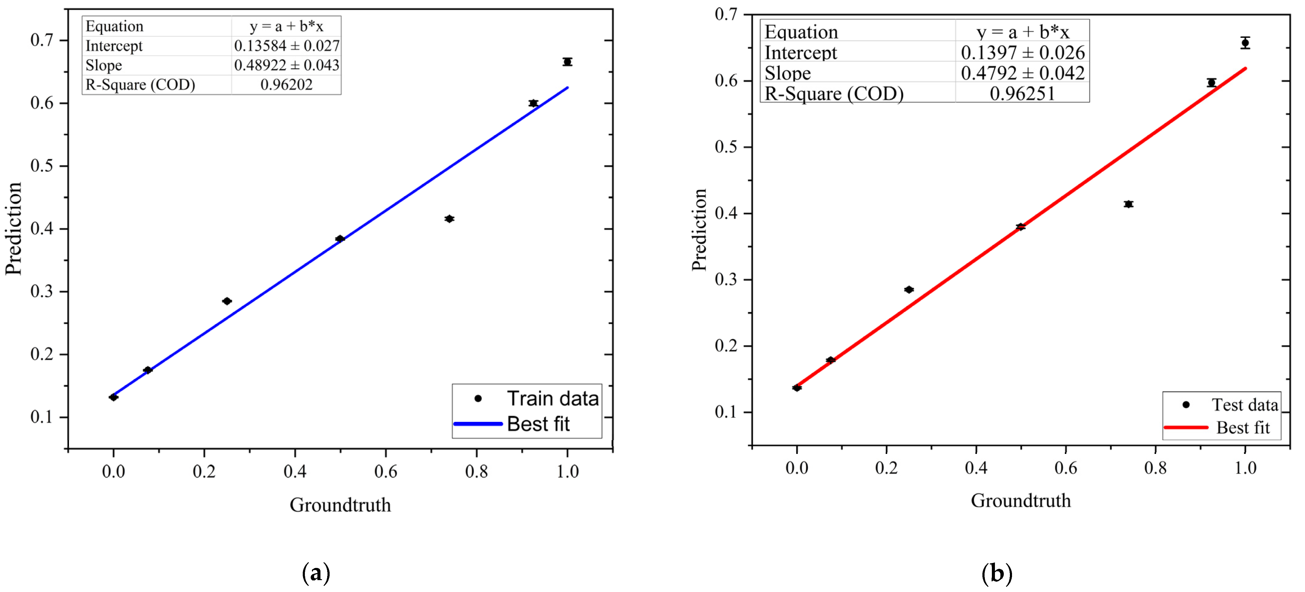
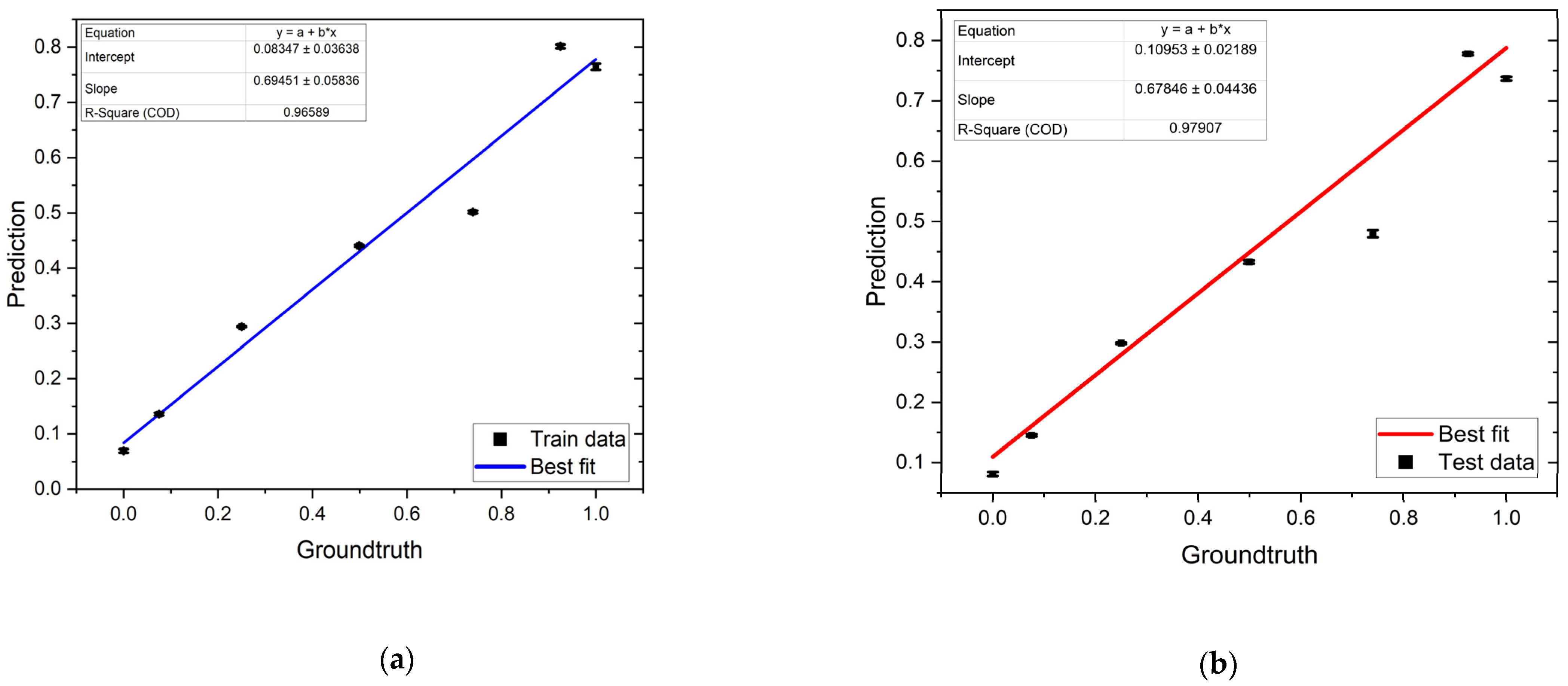
3.3. Regression
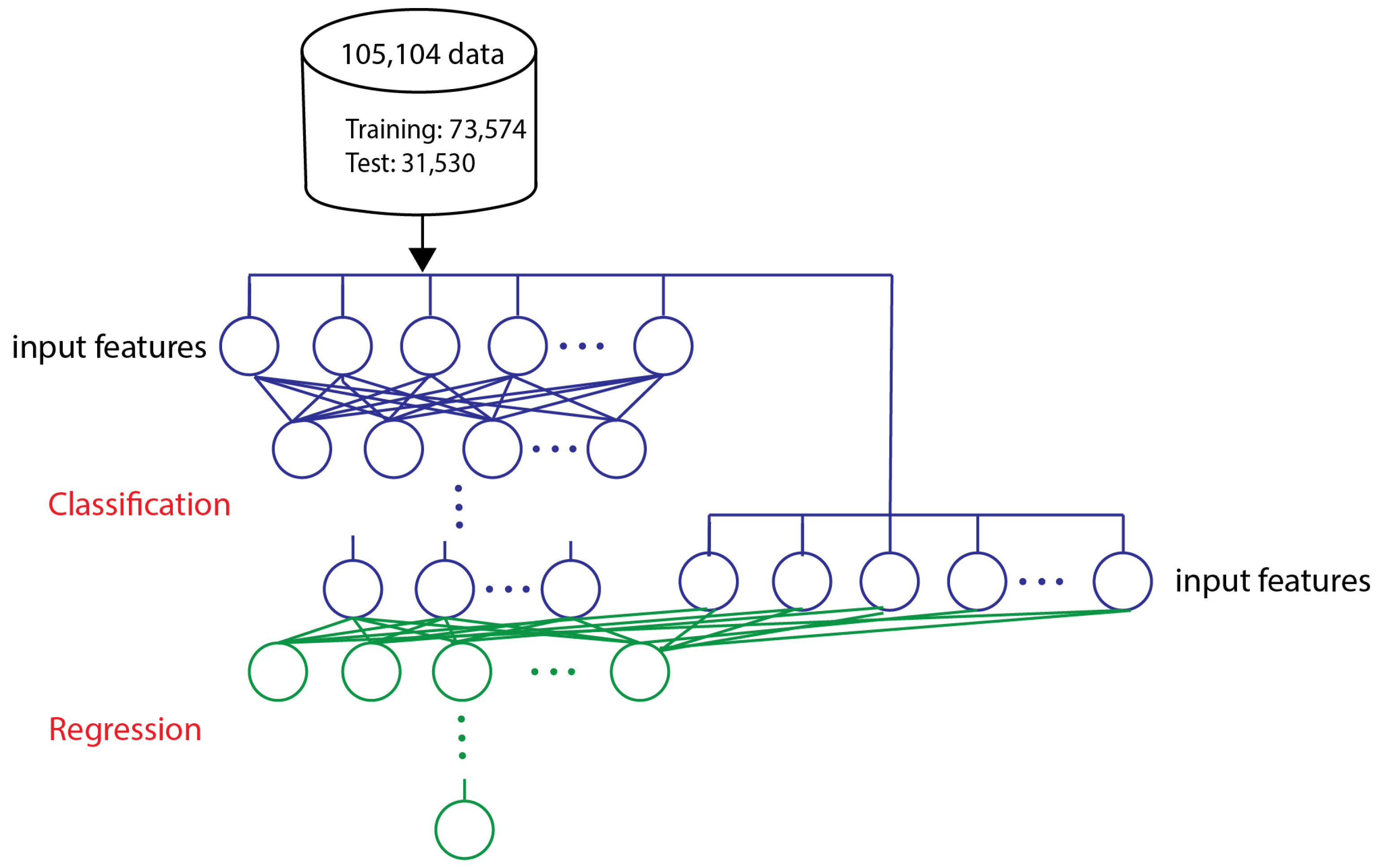
3.4. Hybrid Model
4. Conclusions
Author Contributions
Funding
Institutional Review Board Statement
Informed Consent Statement
Data Availability Statement
Acknowledgments
Conflicts of Interest
References
- Roman, K.; Segal, D. Machine Learning Prediction of DNA Charge Transport. J. Phys. Chem. 2019, 123, 2801–2811. [Google Scholar]
- DNA in Supramolecular Chemistry and Nanotechnology; Stulz, E.; Clever, G.H. (Eds.) John Wiley & Sons: Hoboken, NJ, USA, 2015. [Google Scholar]
- Drummond, T.G.; Hill, M.G.; Barton, J.K. Barton. Electrochemical DNA sensors. Nat. Biotechnol. 2003, 21, 1192–1199. [Google Scholar] [CrossRef] [Green Version]
- Clausen, C.H.; Dimaki, M.; Bertelsen, C.V.; Skands, G.E.; Rodriguez-Trujillo, R.; Thomsen, J.D.; Svendsen, W.E. Bacteria Detection and Differentiation Using Impedance Flow Cytometry. Sensors 2018, 18, 3496. [Google Scholar] [CrossRef] [Green Version]
- Sui, J.; Gandotra, N.; Xie, P.; Lin, Z.; Scharfe, C.; Javanmard, M. Multi-frequency impedance sensing for detection and sizing of DNA fragments. Sci. Rep. 2021, 11, 6490. [Google Scholar] [CrossRef]
- Lin, Z.; Lin, S.Y.; Xie, P.; Lin, C.Y.; Rather, G.M.; Bertino, J.R.; Javanmard, M. Rapid Assessment of Surface Markers on cancer cells Using immuno-Magnetic Separation and Mul-ti-frequency impedance cytometry for targeted therapy. Sci. Rep. 2020, 10, 3015. [Google Scholar] [CrossRef] [Green Version]
- Schoendube, J.; Wright, D.; Zengerle, R.; Koltay, P. Single-cell printing based on impedance detection. Biomicrofluidics 2015, 9, 014117. [Google Scholar] [CrossRef] [Green Version]
- Jung, T.; Yun, Y.R.; Bae, J.; Yang, S. Rapid bacteria-detection platform based on magnetophoretic concentration, dielectrophoretic separation, and impedimetric detection. Anal. Chim. Acta 2021, 1173, 338696. [Google Scholar] [CrossRef]
- Qu, K.; Wei, L.; Zou, Q. A Review of DNA-binding Proteins Prediction Methods. Curr. Bioinform. 2019, 14, 246–254. [Google Scholar] [CrossRef]
- Mok, J.; Mindrinos, M.N.; Davis, R.W.; Javanmard, M. Digital microfluidic assay for protein detection. Proc. Natl. Acad. Sci. USA 2014, 111, 2110–2115. [Google Scholar] [CrossRef] [Green Version]
- Mahmoodi, S.R.; Xie, P.; Zachs, D.P.; Peterson, E.J.; Graham, R.S.; Kaiser, C.R.W.; Lim, H.H.; Allen, M.G.; Javanmard, M. Single-step label-free nanowell immunoassay accurately quantifies serum stress hormones within minutes. Sci. Adv. 2021, 7, eabf4401. [Google Scholar] [CrossRef]
- Furniturewalla, A.; Chan, M.; Sui, J.; Ahuja, K.; Javanmard, M. Fully integrated wearable impedance cytometry platform on flexible circuit board with online smartphone readout. Microsyst. Nanoeng. 2018, 4, 20. [Google Scholar] [CrossRef] [Green Version]
- Xie, P.; Song, N.; Shen, W.; Allen, M.; Javanmard, M. A ten-minute, single step, label-free, sample-to-answer assay for qualitative detection of cytokines in serum at femtomolar levels. Biomed. Microdevices 2020, 22, 73. [Google Scholar] [CrossRef] [PubMed]
- Kokabi, M.; Donnelly, M.; Xu, G. Benchmarking Small-Dataset Structure-Activity-Relationship Models for Prediction of Wnt Signaling Inhibition. IEEE Access 2020, 8, 228831–228840. [Google Scholar] [CrossRef]
- Cruz, J.A.; Wishart, D.S. Applications of Machine Learning in Cancer Prediction and Prognosis. Cancer Inform. 2006, 2, 117693510600200030. [Google Scholar] [CrossRef]
- Gupta, S.; Tran, T.; Luo, W.; Phung, D.; Kennedy, R.L.; Broad, A.; Campbell, D.; Kipp, D.; Singh, M.; Khasraw, M.; et al. Machine-learning prediction of cancer survival: A retrospective study using electronic administrative records and a cancer registry. BMJ Open 2014, 4, e004007. [Google Scholar] [CrossRef] [Green Version]
- Li, J.; Zhou, Z.; Dong, J.; Fu, Y.; Li, Y.; Luan, Z.; Peng, X. Predicting breast cancer 5-year survival using machine learning: A systematic review. PLoS ONE 2021, 16, e0250370. [Google Scholar] [CrossRef]
- Mccarthy, J.F.; Marx, K.A.; Hoffman, P.E.; Gee, A.G.; O’neil, P.; Ujwal, M.L.; Hotchkiss, J. Applications of machine learning and high-dimensional visualization in cancer detection, diagnosis, and management. Ann. N. Y. Acad. Sci. 2004, 1020, 239–262. [Google Scholar] [CrossRef]
- Galan, E.A.; Zhao, H.; Wang, X.; Dai, Q.; Huck, W.T.; Ma, S. Intelligent Microfluidics: The Convergence of Machine Learning and Microfluidics in Materials Science and Biomedicine. Matter 2020, 3, 1893–1922. [Google Scholar] [CrossRef]
- Raji, H.; Tayyab, M.; Sui, J.; Mahmoodi, S.R.; Javanmard, M. Biosensors and machine learning for enhanced detection, stratification, and classification of cells: A review. Biomed. Microdevices 2022, 24, 26. [Google Scholar] [CrossRef]
- Ashley, B.K.; Sui, J.; Javanmard, M.; Hassan, U. Aluminum Oxide-Coated Particle Differentiation Employing Supervised Machine Learning and Impedance Cytometry. In Proceedings of the 2022 IEEE 17th International Conference on Nano/Micro Engineered and Molecular Systems (NEMS), Taoyuan, Taiwan, 14–17 April 2022. [Google Scholar]
- Javanmard, M.; Ahuja, K.; Sui, J.; Bertino, J.R. Use of Multi-Frequency Impedance Cytometry in Conjunction with Machine Learning for Classification of Biological Particles. U.S. Patent Application No. 16/851,580, 2020. [Google Scholar]
- Sui, J.; Gandotra, N.; Xie, P.; Lin, Z.; Scharfe, C.; Javanmard, M. Label-free DNA quantification by multi-frequency impedance cytometry and machine learning analysis. In Proceedings of the 21st International Conference on Miniaturized Systems for Chemistry and Life Sciences, MicroTAS 2017, Savannah, GA, USA, 22–26 October 2017; Chemical and Biological Microsystems Society: Basel, Switzerland, 2020. [Google Scholar]
- Lin, Z.; Sui, J.; Xie, P.; Ahuja, K.; Javanmard, M. A Two-Minute Assay for Electronic Quantification of Antibodies in Saliva Enabled Through Multi-Frequency Impedance Cytometry and Machine Learning Analysis. In 2018 Solid-State Sensors, Actuators and Microsystems Workshop, Hilton Head 2018; Transducer Research Foundation: San Diego, CA, USA, 2018. [Google Scholar]
- Caselli, F.; Reale, R.; De Ninno, A.; Spencer, D.; Morgan, H.; Bisegna, P. Deciphering impedance cytometry signals with neural networks. Lab Chip 2022, 22, 1714–1722. [Google Scholar] [CrossRef]
- Patel, S.K.; Surve, J.; Parmar, J.; Natesan, A.; Katkar, V. Graphene-Based Metasurface Refractive Index Biosensor For Hemoglobin Detection: Machine Learning Assisted Optimization. IEEE Trans. NanoBioscience 2022, 1. [Google Scholar] [CrossRef]
- Schuett, J.; Bojorquez, D.I.S.; Avitabile, E.; Mata, E.S.O.; Milyukov, G.; Colditz, J.; Delogu, L.G.; Rauner, M.; Feldmann, A.; Koristka, S.; et al. Nanocytometer for smart analysis of peripheral blood and acute myeloid leukemia: A pilot study. Nano Lett. 2020, 20, 6572–6581. [Google Scholar] [CrossRef] [PubMed]
- Honrado, C.; Salahi, A.; Adair, S.J.; Moore, J.H.; Bauer, T.W.; Swami, N.S. Automated biophysical classification of apoptotic pancreatic cancer cell subpopulations by using machine learning approaches with impedance cytometry. Lab Chip 2022, 22, 3708–3720. [Google Scholar] [CrossRef] [PubMed]
- Ahuja, K.; Rather, G.M.; Lin, Z.; Sui, J.; Xie, P.; Le, T.; Bertino, J.R.; Javanmard, M. Toward point-of-care assessment of patient response: A portable tool for rapidly assessing cancer drug efficacy using multifrequency impedance cytometry and supervised machine learning. Microsyst. Nanoeng. 2019, 5, 34. [Google Scholar] [CrossRef] [PubMed] [Green Version]
- Feng, Y.; Cheng, Z.; Chai, H.; He, W.; Huang, L.; Wang, W. Neural network-enhanced real-time impedance flow cytometry for single-cell intrinsic characterization. Lab Chip 2022, 22, 240–249. [Google Scholar] [CrossRef]
- Sui, J.; Xie, P.; Lin, Z.; Javanmard, M. Electronic classification of barcoded particles for multiplexed detection using supervised machine learning analysis. Talanta 2020, 215, 120791. [Google Scholar] [CrossRef] [PubMed]
- Nabipour, M.; Nayyeri, P.; Jabani, H.; Shahab, S.; Mosavi, A. Predicting Stock Market Trends Using Machine Learning and Deep Learning Algorithms Via Continuous and Binary Data; A Comparative Analysis. IEEE Access 2020, 8, 150199–150212. [Google Scholar] [CrossRef]
- Zhang, M.; Ye, J.; He, J.-S.; Zhang, F.; Ping, J.; Qian, C.; Wu, J. Visual detection for nucleic acid-based techniques as potential on-site detection methods. A review. Anal. Chim. Acta 2020, 1099, 1–15. [Google Scholar] [CrossRef]
- Nayak, S.C.; Misra, B.B.; Behera, H.S. Impact of data normalization on stock index forecasting. Int. J. Comput. Inf. Syst. Ind. Manag. Appl. 2014, 6, 257–269. [Google Scholar]
- Wong, K.I.; Wong, P.K.; Cheung, C.S.; Vong, C.M. Modeling and optimization of biodiesel engine performance using advanced machine learning methods. Energy 2013, 55, 519–528. [Google Scholar] [CrossRef]
- Eesa, A.S.; Arabo, W.K. A Normalization Methods for Backpropagation: A Comparative Study. Sci. J. Univ. Zakho 2017, 5, 319–323. [Google Scholar] [CrossRef] [Green Version]
- Kumar, S.; Nancy. Efficient K-Mean Clustering Algorithm for Large Datasets using Data Mining Standard Score Normalization. Int. J. Recent Innov. Trends Comput. Commun. 2014, 2, 3161–3166. [Google Scholar]
- Pires, I.M.; Hussain, F.; Garcia, N.M.M.; Lameski, P.; Zdravevski, E. Homogeneous Data Normalization and Deep Learning: A Case Study in Human Activity Classification. Futur. Internet 2020, 12, 194. [Google Scholar] [CrossRef]
- Borkin, D.; Némethová, A.; Michaľčonok, G.; Maiorov, K. Impact of data normalization on classification model accuracy. Res. Pap. Fac. Mater. Sci. Technol. Slovak Univ. Technol. 2019, 27, 79–84. [Google Scholar] [CrossRef] [Green Version]
- Fahami, M.A.; Roshanzamir, M.; Izadi, N.H.; Keyvani, V.; Alizadehsani, R. Detection of effective genes in colon cancer: A machine learning approach. Inform. Med. Unlocked 2021, 24, 100605. [Google Scholar] [CrossRef]
- Kassani, S.H.; Kassani, P.H.; Wesolowski, M.J.; Schneider, K.A.; Deters, R. Classification of Histopathological Biopsy Images Using Ensemble of Deep Learning Networks. arXiv 2019, arXiv:1909.11870. [Google Scholar]
- Wong, K.I.; Wong, P.K.; Cheung, C.S.; Vong, C.M. Modelling of diesel engine performance using advanced machine learning methods under scarce and exponential data set. Appl. Soft Comput. 2013, 13, 4428–4441. [Google Scholar] [CrossRef]
- Pedregosa, F.; Varoquaux, G.; Gramfort, A.; Michel, V.; Thirion, B.; Grisel, O.; Blondel, M.; Prettenhofer, P.; Weiss, R.; Dubourg, V.; et al. Scikit-learn: Machine learning in Python. J. Mach. Learn. Res. 2011, 12, 2825–2830. [Google Scholar]
- Liaqat, S.; Dashtipour, K.; Arshad, K.; Assaleh, K.; Ramzan, N. A Hybrid Posture Detection Framework: Integrating Machine Learning and Deep Neural Networks. IEEE Sens. J. 2021, 21, 9515–9522. [Google Scholar] [CrossRef]
- Satu, M.S.; Howlader, K.C.; Mahmud, M.; Kaiser, M.S.; Shariful Islam, S.M.; Quinn, J.M.; Alyamit, S.A.; Moni, M.A. Short-term prediction of COVID-19 cases using machine learning models. Appl. Sci. 2021, 11, 4266. [Google Scholar] [CrossRef]
- Panchal, G.; Ganatra, A.; Kosta, Y.P.; Panchal, D. Behaviour analysis of multilayer perceptrons with multiple hidden neurons and hidden layers. Int. J. Comput. Theory Eng. 2011, 3, 332–337. [Google Scholar] [CrossRef] [Green Version]
- James, B.; Bengio, Y. Random search for hyper-parameter optimization. J. Mach. Learn. Res. 2012, 13, 281–305. [Google Scholar]
- Snoek, J.; Larochelle, H.; Adams, R.P. Practical bayesian optimization of machine learning algorithms. Adv. Neural Inf. Process. Syst. 2012, 2, 2951–2959. [Google Scholar]
- Hasebrook, N.; Morsbach, F.; Kannengießer, N.; Franke, J.; Hutter, F.; Sunyaev, A. Why Do Machine Learning Practitioners Still Use Manual Tuning? A Qualitative Study. arXiv 2022, arXiv:2203.01717. [Google Scholar]
- Ying, X. An Overview of Overfitting and its Solutions. J. Phys. Conf. Ser. 2019, 1168, 022022. [Google Scholar] [CrossRef]
- Chieregato, M.; Frangiamore, F.; Morassi, M.; Baresi, C.; Nici, S.; Bassetti, C.; Bnà, C.; Galelli, M. A hybrid machine learning/deep learning COVID-19 severity predictive model from CT images and clinical data. Sci. Rep. 2022, 12, 4329. [Google Scholar] [CrossRef] [PubMed]
- Gavrishchaka, V.; Yang, Z.; Miao, R.; Senyukova, O. Advantages of hybrid deep learning frameworks in applications with limited data. Int. J. Mach. Learn. Comput. 2018, 8, 549–558. [Google Scholar]


| DNA Length | DNA Amount per Bead |
|---|---|
| Bare bead | 0 |
| 300 bp | |
| 300 bp | |
| 300 bp | |
| 300 bp | |
| 300 bp | |
| 300 bp |
| Model Number | Number of Hidden Layers | Number of Neurons in Each Layer |
|---|---|---|
| 1 | 2 | 10,10 |
| 2 | 2 | 20,20 |
| 3 | 3 | 20,20,10 |
| 4 | 3 | 30,20,10 |
| 5 | 4 | 40,30,20,10 |
| 6 | 5 | 60,50,30,20,10 |
| 7 | 5 | 70,50,40,20,10 |
| 8 | 5 | 80,60,40,30,20 |
| 9 | 6 | 100,80,60,50,20,10 |
| 10 | 6 | 100,80,80,60,30,20 |
| 1 | 2 | 3 | 4 | 5 | 6 | 7 | |
|---|---|---|---|---|---|---|---|
| ACC | 0.97 | 0.91 | 0.89 | 0.89 | 0.88 | 0.97 | 0.97 |
| TPR | 0.43 | 0.87 | 0.80 | 0.87 | 0.51 | 0.8 | 0.78 |
| TNR | 0.99 | 0.92 | 0.92 | 0.89 | 0.93 | 0.99 | 0.99 |
| FPR | 0.004 | 0.07 | 0.07 | 0.10 | 0.06 | 0.07 | 0.09 |
| FNR | 0.56 | 0.12 | 0.19 | 0.12 | 0.48 | 0.99 | 0.21 |
| Model | MSE Train | MSE Test | Train (%) | Test (%) |
|---|---|---|---|---|
| 1 | 0.3077 | 0.3077 | 67.61 | 67.98 |
| 2 | 0.2959 | 0.2954 | 57.34 | 56.83 |
| 3 | 0.2821 | 0.2873 | 72.64 | 71.26 |
| 4 | 0.2796 | 0.2811 | 75.39 | 74.76 |
| 5 | 0.2615 | 0.2786 | 90.69 | 90.6 |
| 6 | 0.2286 | 0.2481 | 93.34 | 93.13 |
| 7 | 0.2281 | 0.2373 | 91.89 | 92.16 |
| 8 | 0.2254 | 0.232 | 96.2 | 96.25 |
| 9 | 0.2117 | 0.2338 | 94.01 | 94.29 |
| 10 | 0.2087 | 0.2198 | 95.23 | 95.07 |
Disclaimer/Publisher’s Note: The statements, opinions and data contained in all publications are solely those of the individual author(s) and contributor(s) and not of MDPI and/or the editor(s). MDPI and/or the editor(s) disclaim responsibility for any injury to people or property resulting from any ideas, methods, instructions or products referred to in the content. |
© 2023 by the authors. Licensee MDPI, Basel, Switzerland. This article is an open access article distributed under the terms and conditions of the Creative Commons Attribution (CC BY) license (https://creativecommons.org/licenses/by/4.0/).
Share and Cite
Kokabi, M.; Sui, J.; Gandotra, N.; Pournadali Khamseh, A.; Scharfe, C.; Javanmard, M. Nucleic Acid Quantification by Multi-Frequency Impedance Cytometry and Machine Learning. Biosensors 2023, 13, 316. https://doi.org/10.3390/bios13030316
Kokabi M, Sui J, Gandotra N, Pournadali Khamseh A, Scharfe C, Javanmard M. Nucleic Acid Quantification by Multi-Frequency Impedance Cytometry and Machine Learning. Biosensors. 2023; 13(3):316. https://doi.org/10.3390/bios13030316
Chicago/Turabian StyleKokabi, Mahtab, Jianye Sui, Neeru Gandotra, Arastou Pournadali Khamseh, Curt Scharfe, and Mehdi Javanmard. 2023. "Nucleic Acid Quantification by Multi-Frequency Impedance Cytometry and Machine Learning" Biosensors 13, no. 3: 316. https://doi.org/10.3390/bios13030316