

Composite Mould Design with Multiphysics FEM Computations Guidance


Abstract
:1. Introduction
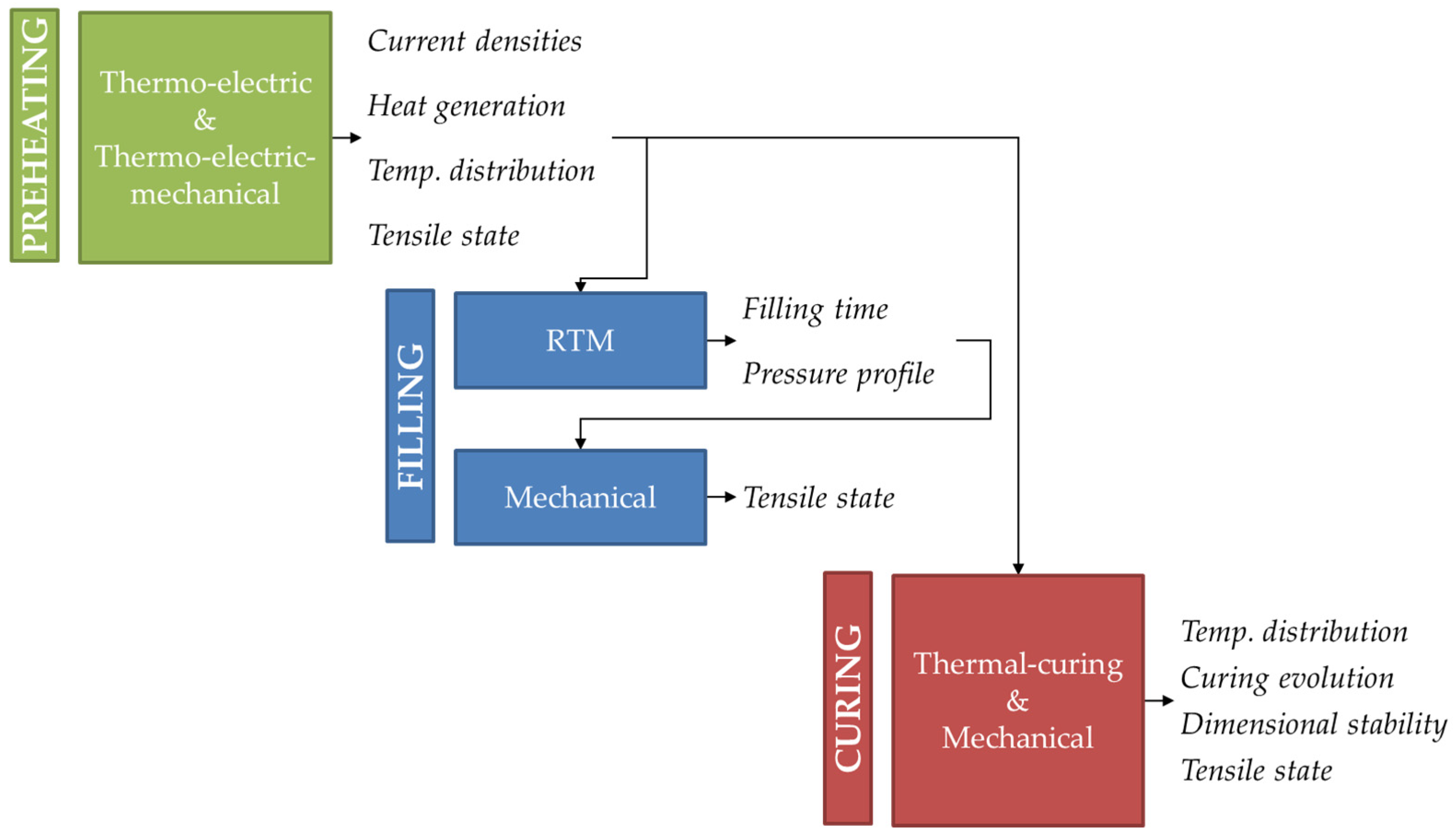
2. Methodology
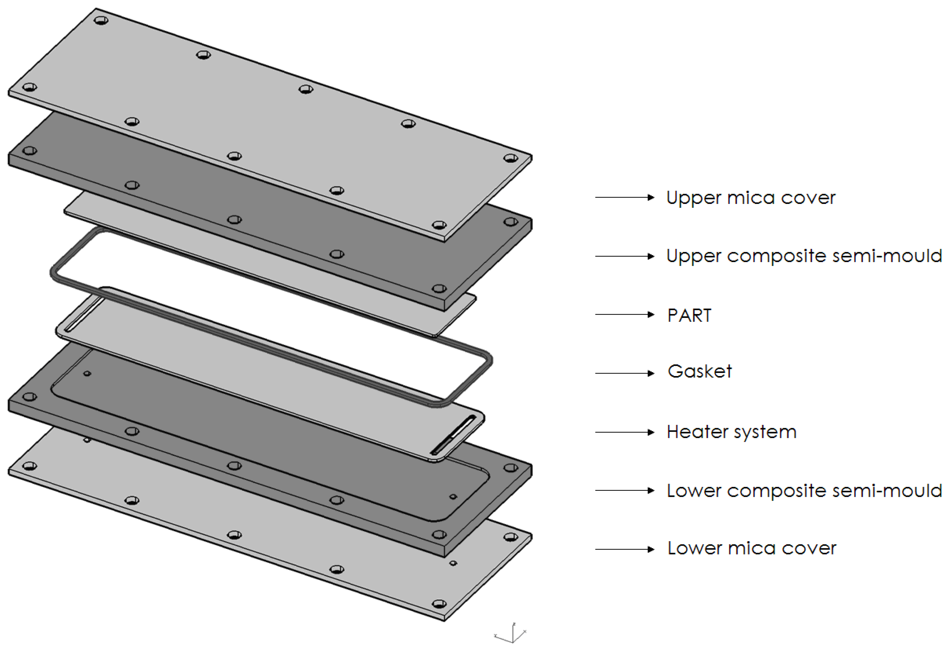
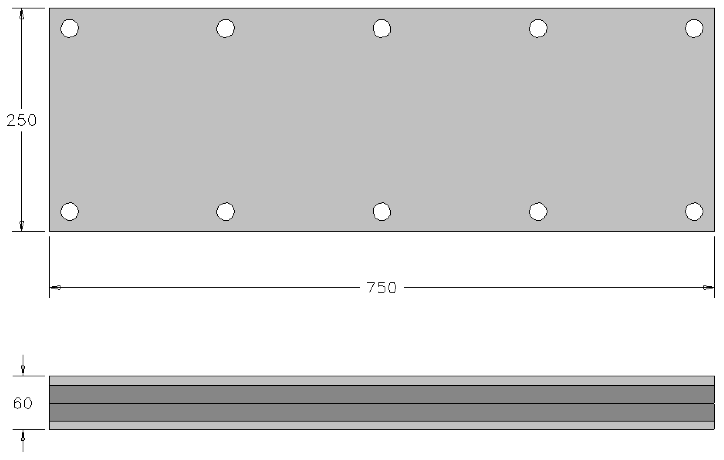
3. Mould Design
4. Results and Discussion
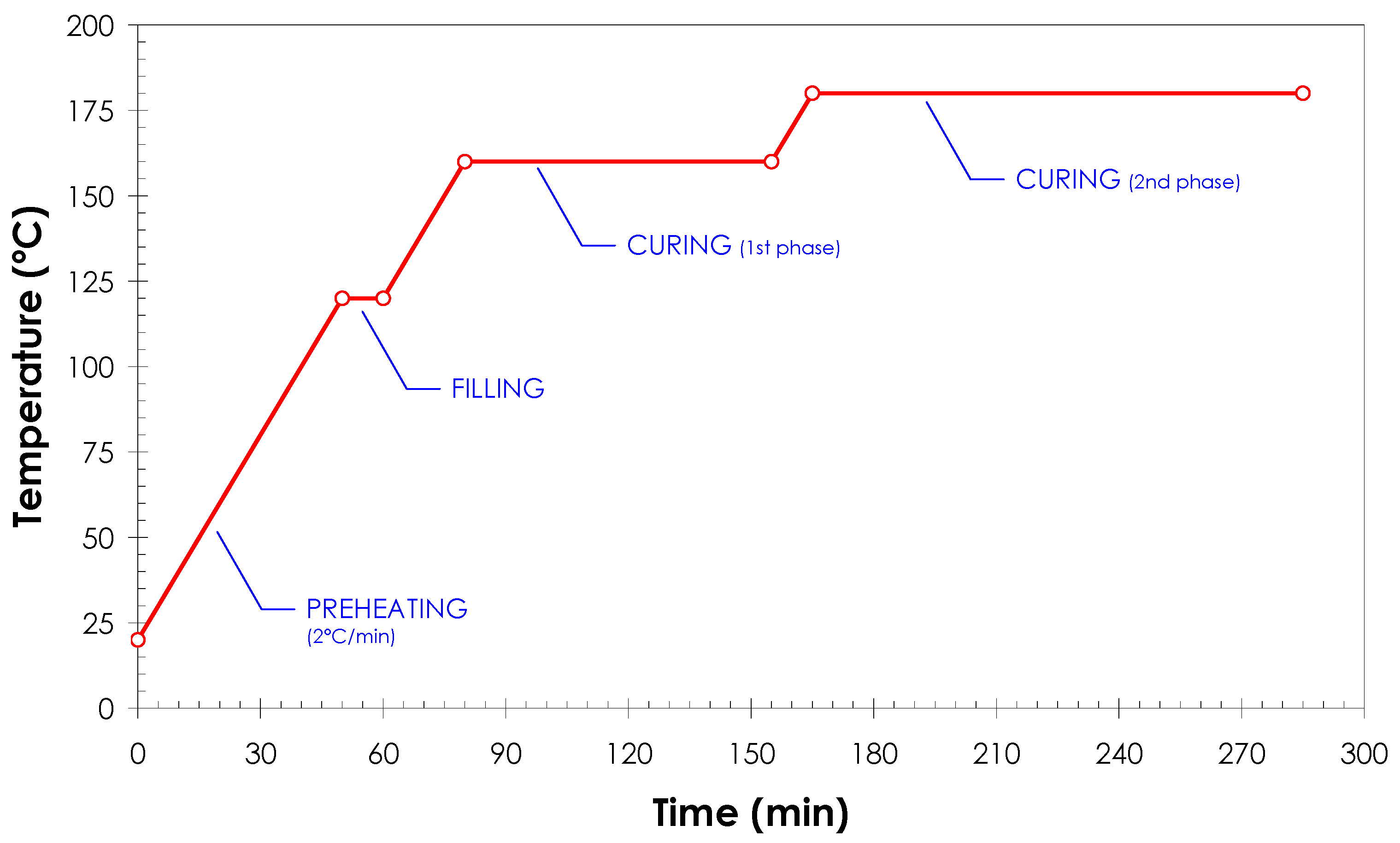
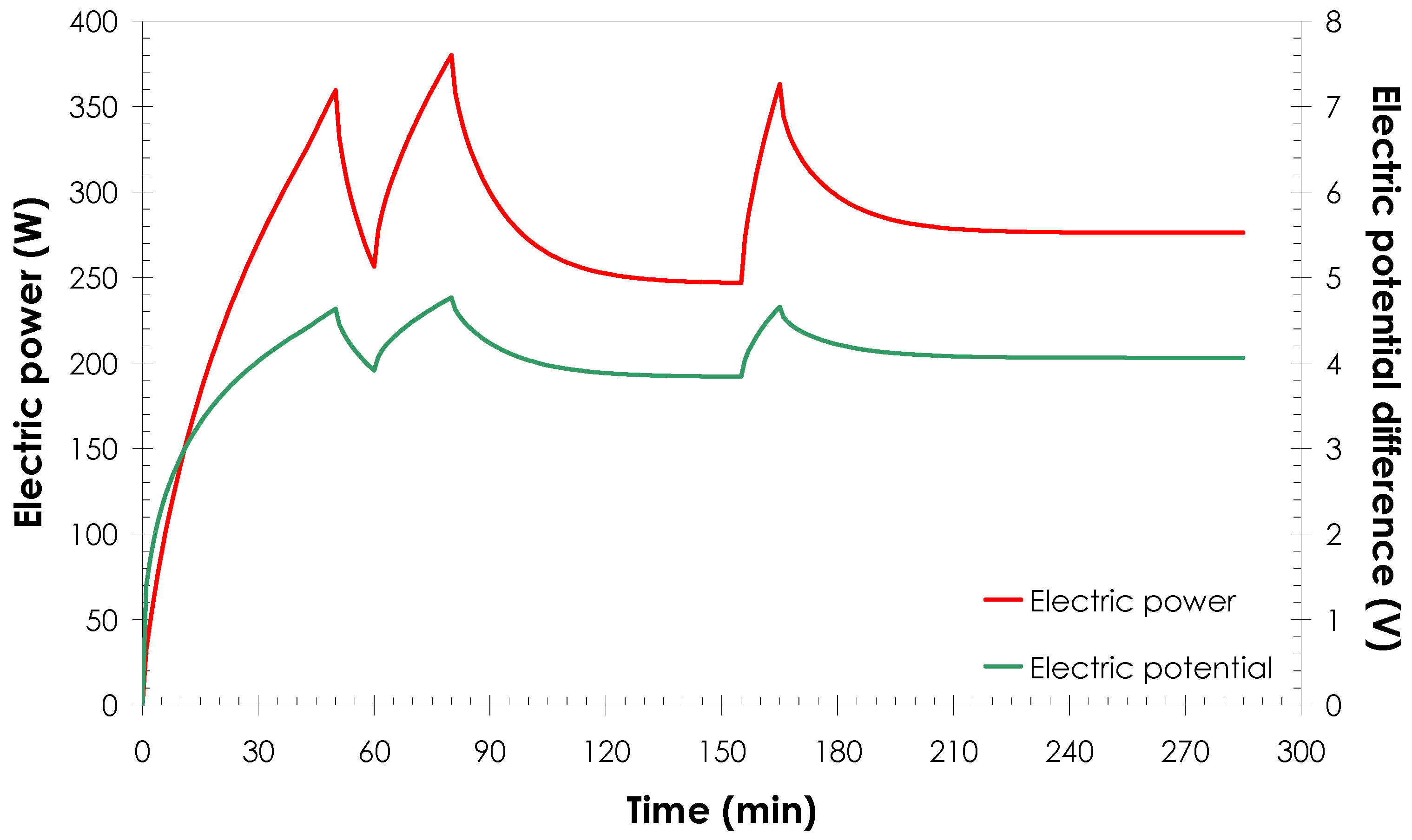
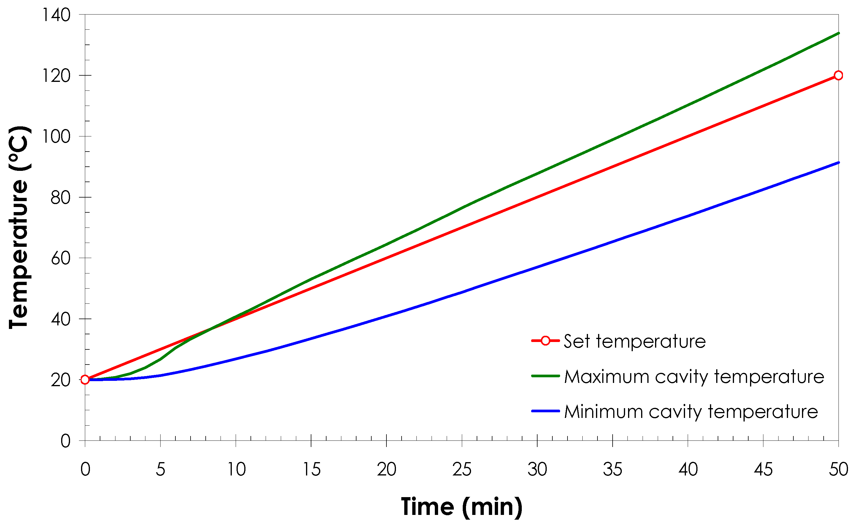
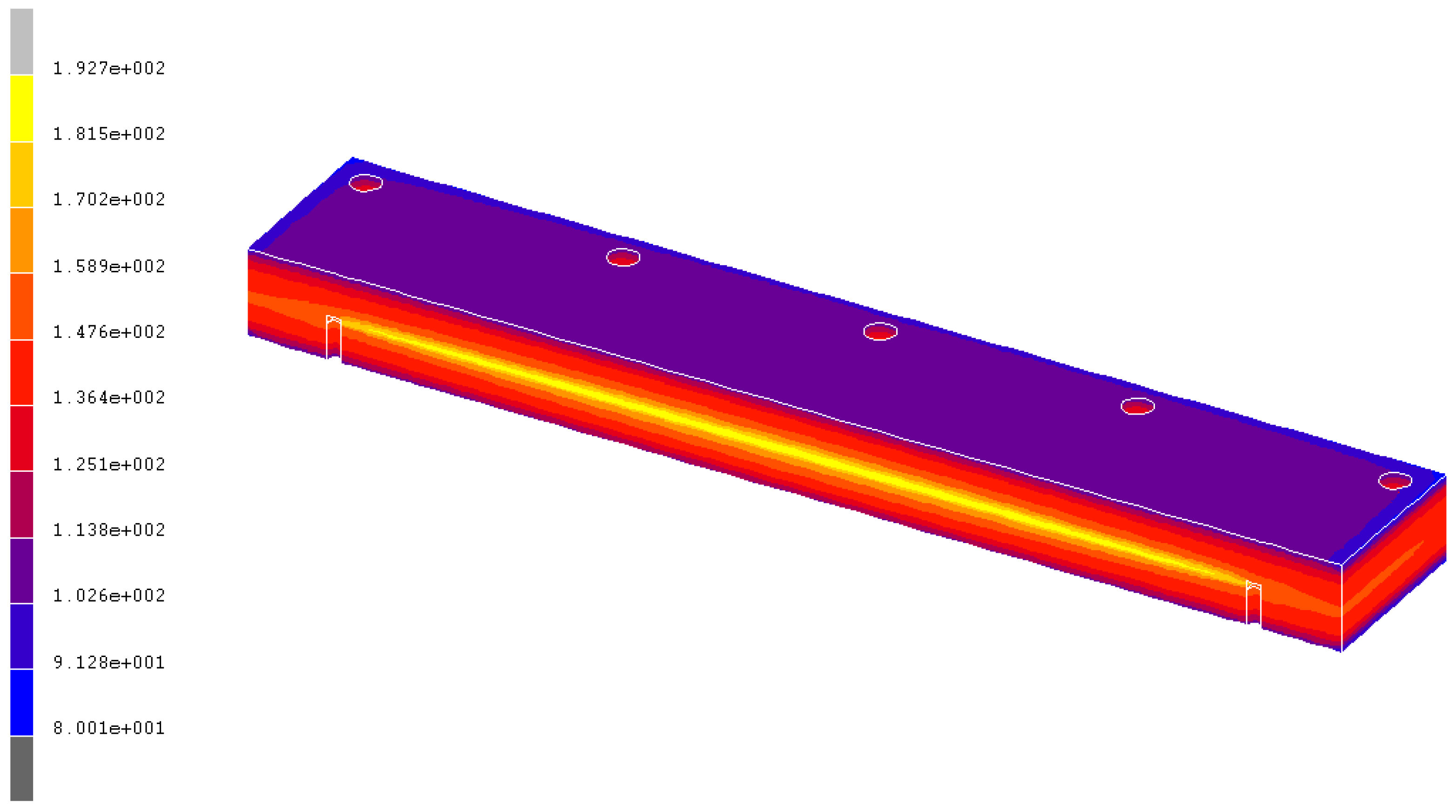
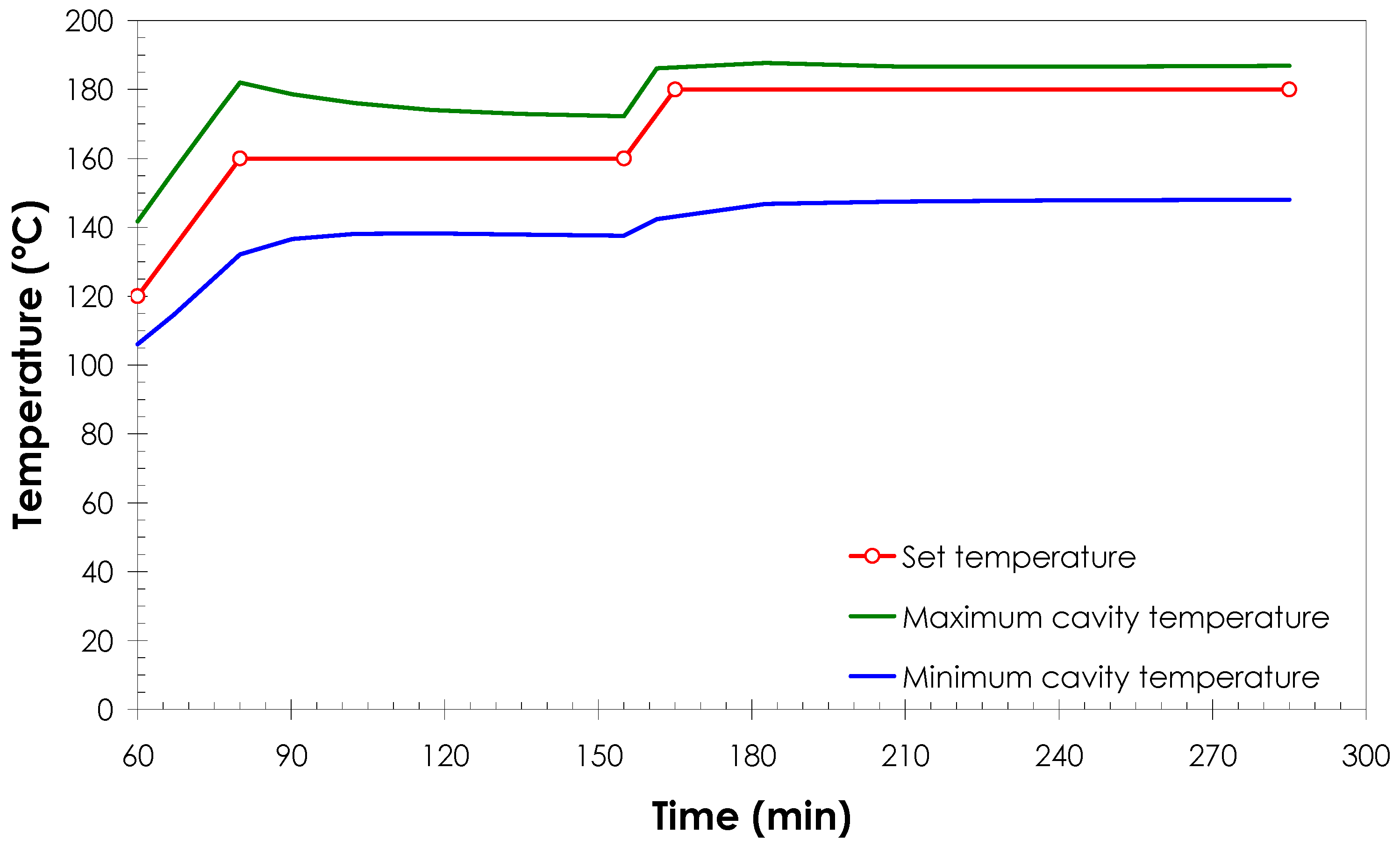
4.1. Preheating
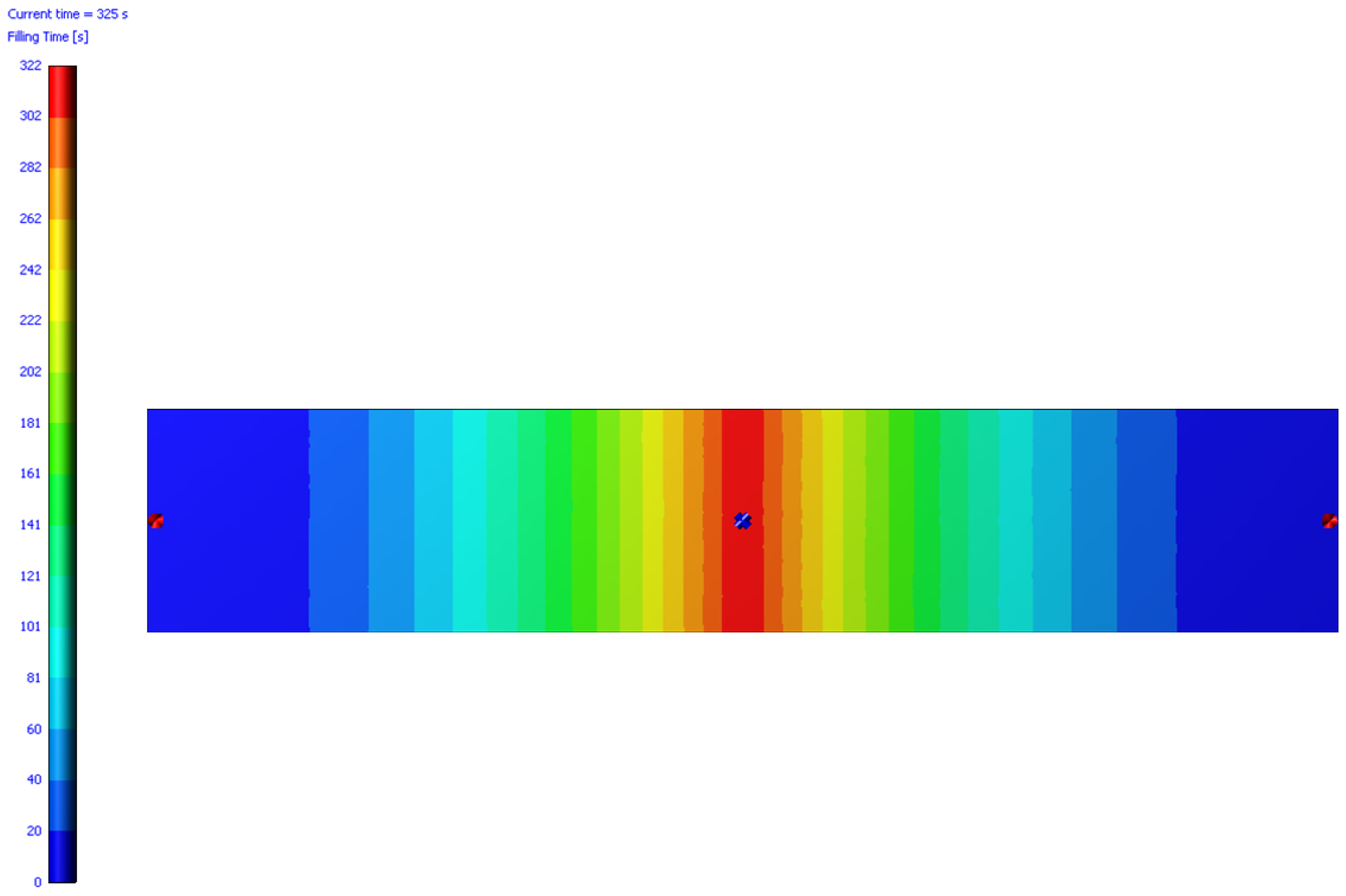
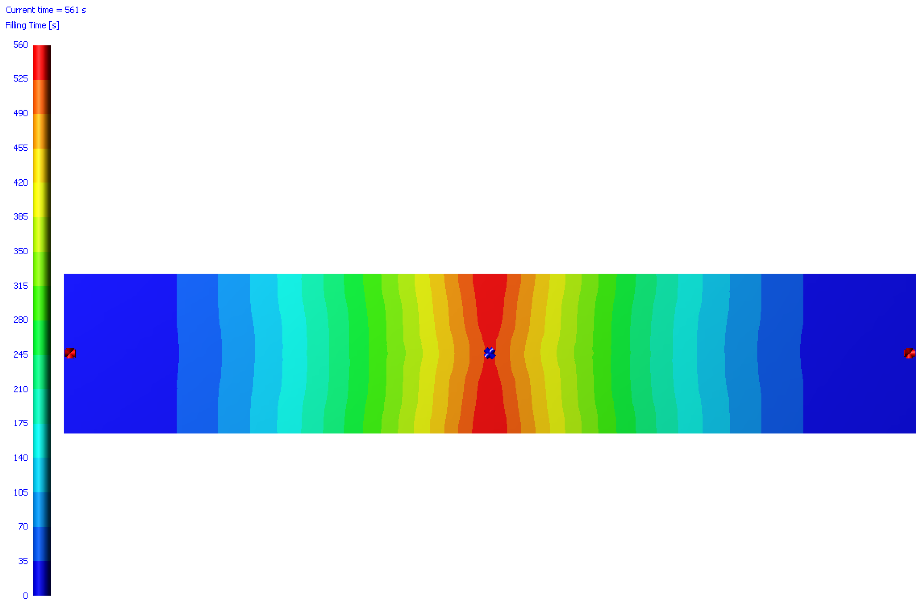
4.2. Filling of the Mould
4.2.1. RTM Process Simulation Considering a Constant Mould Temperature of 120 °C
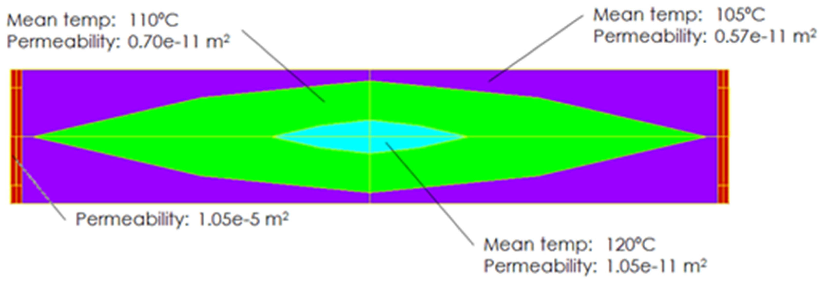
4.2.2. RTM Process Simulation Considering Non-Constant Mould Temperatures
4.3. Curing of the Component
5. Conclusions
- A suitable dielectric material, such as fibreglass, around the resistive heater is needed to minimize electric current to the outer surfaces and to, consequently, avoid the risk of electrocution.
- Appropriate thermal insulation is recommended to minimize heat flows to the adjoining components and, therefore, to reduce the electric energy consumption.
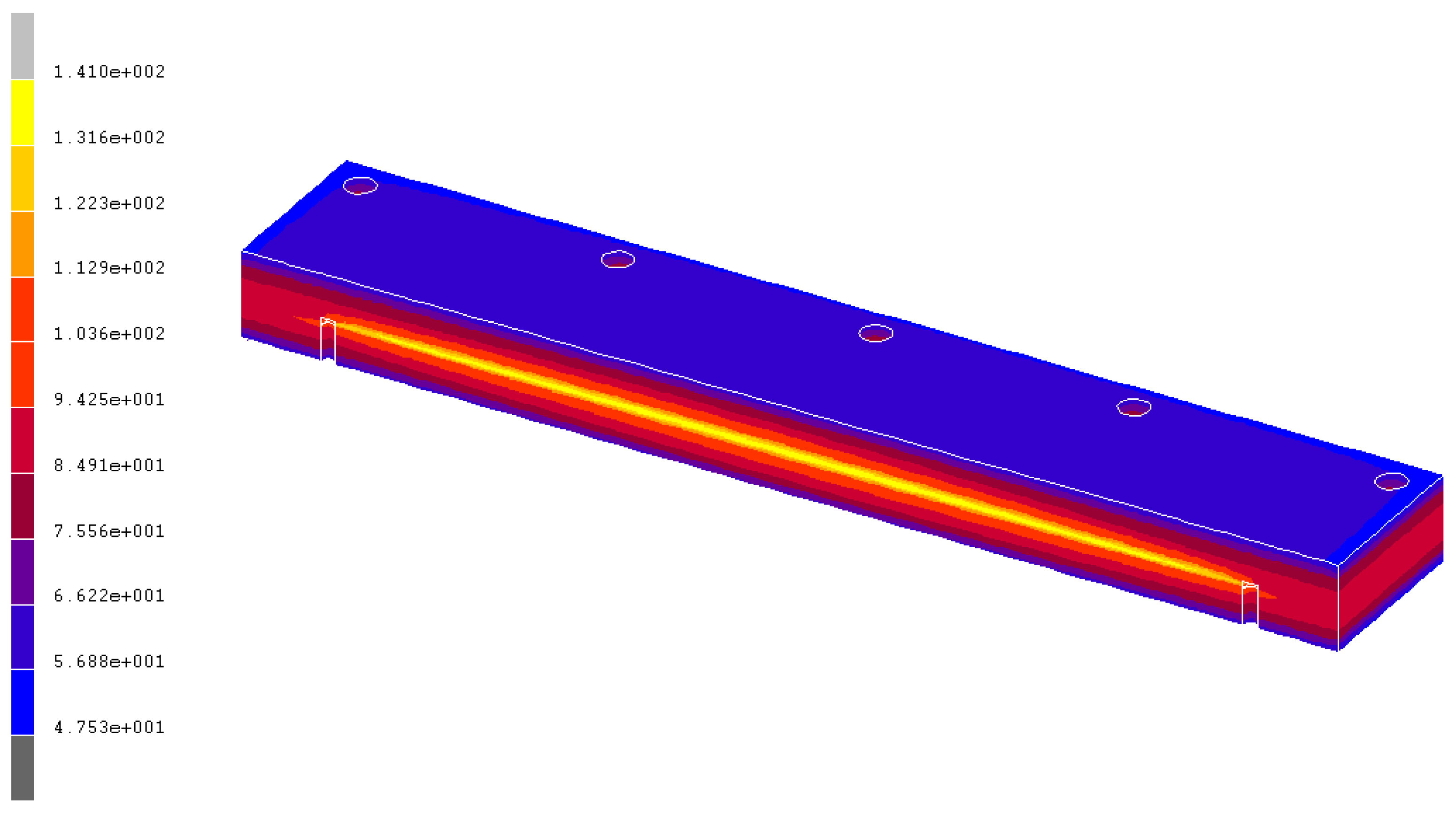
- The temperature distribution reached in the cavity is not uniform (temperature uniformity was desired in the cavity), meaning heating alternatives should be found. A solution could be devised with heaters with variable electric resistances in different zones, but this is a point to be further investigated.
- Due to the temperature dependency of the resin properties, the expected temperature distribution should be considered when the injection strategy of a mould is studied. That way, zones of highest temperatures should be filled at the end of the process if a faster filling is desired.
- Materials of similar CTE’s should be used when possible in order to minimize the stresses and displacements generated. Such parameters could be critical in cases of large CTE mismatches.
- Neither the stresses nor the displacements caused due to the internal pressure from the filling process are expected to be critical with the present design.
- Significant differences in resulting temperatures of up to 10% were found in the preheating stage depending on the analysis type conducted (thermo-electric or thermo-electric–mechanical). Several trials were made and it was concluded that such differences were not generated because of the deformations, but due to the internal formulation used by each analysis. An additional thermal analysis demonstrated that the results from the thermo-electric analysis are more accurate.
- Curing parameters cannot be obtained when electric loads are applied. Therefore, it is concluded that a common heat transfer analysis (assuming the Joule’s effect through an internal heat generation) is required.
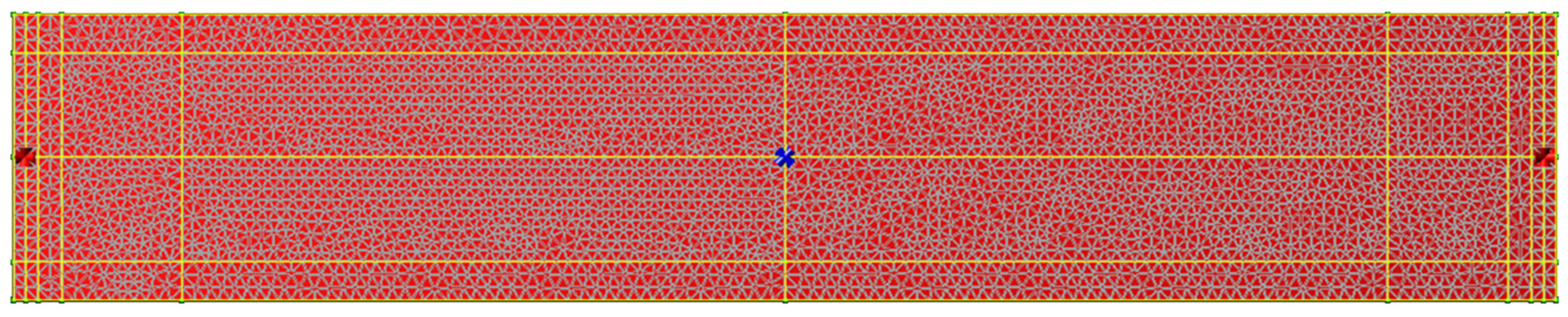
- Only two-dimensional analyses can be performed. However, this may not be critical as thin samples are usually manufactured by RTM.
- Since just linear triangular elements can be used, different meshes have been built in RTM-Worx and, therefore, problems to exchange data/results with MSC-Marc have been found.
- Only isothermal conditions can be considered. Thus, the viscosity of the resin is defined as a constant and, consequently, thermal effects cannot be analysed directly. However, a simple way to take into account the resin temperature dependency by defining different permeability values in the model through real permeability/viscosity ratios has been found.
Author Contributions
Funding
Data Availability Statement
Conflicts of Interest
References
- Trollman, H.; Trollman, F. A Sustainability Assessment of Smart Innovations for Mass Production, Mass Customization and Direct Digital Manufacturing. In Mass Production Processes; Akdogan, A., Vanli, A.S., Eds.; IntechOpen: London, UK, 2019. [Google Scholar] [CrossRef] [Green Version]
- Matvienko, O.; Daneyko, O.; Kovalevskaya, T.; Khrustalyov, A.; Zhukov, I.; Vorozhtsov, A. Investigation of Stresses Induced Due to the Mismatch of the Coefficients of Thermal Expansion of the Matrix and the Strengthening Particle in Aluminum-Based Composites. Metals 2021, 11, 279. [Google Scholar] [CrossRef]
- Zade, A.; Neogi, S.; Kuppusamy, R.R.P. Design of effective injection strategy and operable cure window for an aircraft wing flap composite part using neat resin characterization and multi-physics process simulation. Polym. Compos. 2022, 43, 3426. [Google Scholar] [CrossRef]
- Joo, S.J.; Yu, M.H.; Seock Kim, W.; Lee, J.W.; Kim, H.S. Design and manufacture of automotive composite front bumper assemble component considering interfacial bond characteristics between over-molded chopped glass fiber polypropylene and continuous glass fiber polypropylene composite. Compos. Struct. 2020, 236, 111849. [Google Scholar] [CrossRef]
- Simacek, P.; Advani, S.G.; Iobst, S.A. Modeling Flow in Compression Resin Transfer Molding for Manufacturing of Complex Lightweight High-Performance Automotive Parts. J. Compos. Mater. 2008, 42, 2523–2545. [Google Scholar] [CrossRef]
- Kuppusamy, R.R.P.; Neogi, S. Simulation of air entrapment and resin curing during manufacturing of composite cab front by resin transfer moulding process. Arch. Metall. Mater. 2017, 62, 1839–1844. [Google Scholar] [CrossRef] [Green Version]
- Xiong, F.; Wang, D.; Ma, Z.; Chen, S.; Lv, T.; Lu, F. Structure-material integrated multi-objective lightweight design of the front end structure of automobile body. Struct. Multidiscip. Optim. 2018, 57, 829–847. [Google Scholar] [CrossRef]
- Mal, O.; Couniot, A.; Dupret, F. Non isothermal simulation of the resin transfer moulding press. Compos. Part A Appl. Sci. Manuf. 1998, 29, 189–198. [Google Scholar] [CrossRef]
- Garmendia, I.; Vallejo, H.; Iriarte, A.; Anglada, E. Direct Resistive Heating Simulation Tool for the Repair of Aerospace Structures through Composite Patches. Math. Probl. Eng. 2018, 2018, 4136795. [Google Scholar] [CrossRef] [Green Version]
- Volume A: Theory and User Information; Msc-Marc 2008R1; Msc Software: Newport Beach, CA, USA, 2008.
- RTM-Worxs v2.8, Users Documentation. Available online: https://www.polyworx.com/doc/ (accessed on 8 December 2022).
- Yi, S.; Hilton, H.H.; Ahmad, M.F. A finite element approach for cure simulation of thermosetting matrix composites. Comput. Struct. 1997, 64, 383–388. [Google Scholar] [CrossRef]
- Kim, J.; Moon, T.J.; Howell, J.R. Cure Kinetic Model, Heat of Reaction, and Glass Transition Temperature of AS4/3501-6 Graphite–Epoxy Prepregs. J. Compos. Mater. 2002, 36, 2479–2498. [Google Scholar] [CrossRef]
- Rider, A.N.; Wang, C.H.; Cao, J. Internal resistance heating for homogeneous curing of adhesively bonded repairs. Int. J. Adhes. Adhes. 2011, 31, 168–176. [Google Scholar] [CrossRef]
- Maguire, J.M.; Sharp, N.D.; Pipes, R.B.; Bradaigh, C.M. Advanced process simulations for thick-section epoxy powder composite structures. Compos. Part A 2022, 161, 107073. [Google Scholar] [CrossRef]
- Kenny, J.M.; Maffezzoli, A.M.; Nicolais, L.; Mazzola, M. A model for the thermal and chemorheological behavior of thermoset processing: II) Unsaturated polyester based composites. Compos. Sci. Technol. 1990, 38, 339–358. [Google Scholar] [CrossRef]


| Property | Composite | Rubber | Mica | Fiberglass | Dry Fibre | Resin | Composite Part |
|---|---|---|---|---|---|---|---|
| Density (kg/m3) | 1700 | 1150 | 2850 | 1800 | 1790 | 1150 | 1500 |
| Electrical resistivity (ohm·m) | |||||||
| xx | 5.88 × 10⁻⁶ | 5.88 × 10⁻⁶ | |||||
| yy | 5.88 × 10⁻⁶ | 1 × 10¹⁴ | 2 × 10¹³ | 1 × 10¹⁴ | 5.88 × 10⁻⁶ | NC | NC |
| zz | 5.88 × 10⁻⁴ | 5.88 × 10⁻⁵ | |||||
| Thermal conductivity W/(m·K) | |||||||
| xx | 164 | 6.83 | 7 | ||||
| yy | 164 | 0.15 | 0.35 | 0.58 | 6.83 | 0.3 | 7 |
| zz | 1 | 0.683 | 1 | ||||
| Specific heat J/(kg·K) | 500 | 2000 | 880 | 795 | 1130 | 1500 | 1300 |
| CTE (1/C), ×10−6 | |||||||
| xx | 1 × 10⁻³ | ||||||
| yy | 1 × 10⁻³ | 80 | 10 | 8 | NC | NC | NC |
| zz | 50 | ||||||
| Emissivity | 0.9 | - | 0.75 | - | - | - | - |
| Young’s modulus (GPa) | |||||||
| xx | 150 | ||||||
| yy | 150 | 7 × 10⁻³ | 172 | 18 | NC | NC | NC |
| zz | 4 | ||||||
| Poisson’s ratio | |||||||
| xy | 0.2 | ||||||
| yz | 0.015 | 0.495 | 0.3 | 0.3 | NC | NC | NC |
| xz | 0.015 | ||||||
| Transv. elasticity modulus (GPa) | |||||||
| xy | 62 | ||||||
| yz | 2.75 | - | - | - | - | - | - |
| xz | 2.75 | ||||||
| Viscosity (mPa·s) at 120 °C | - | - | - | - | - | 33 | - |
| Permeability (m2), ×10−11 | |||||||
| xx | - | - | - | - | - | 1.05 | - |
| yy | - | - | - | - | - | 1.05 | - |
| Coefficient | Value | Coefficient | Value |
|---|---|---|---|
| A1 | 1451.873 s−1 | Hr | 480,000 J/kg |
| A2 | 16,797.24 s−1 | b1 | 1.04578 |
| ΔE1 | 7739.757 J/mol | b2 | −7.9 × 10⁻⁴ K−1 |
| ΔE2 | 7725.694 J/mol | b3 | 1.4708 × 10⁻⁶ K−2 |
| m1 | 0.75079 | n1 | −1.44997 |
| m2 | 2.4 × 10⁻⁴ K−1 | n2 | 0.0606 K−1 |
| m3 | 4.4432 × 10⁻⁷ K−2 | n3 | −7.6515 × 10⁻⁷ K−2 |
| Location | Max. Von Mises Stress (MPa) | Max. Displacement (mm) |
|---|---|---|
| Upper mica cover | 125 | 0.20 |
| Upper composite mould | 110 | 0.19 |
| Sample | 0 | 0.14 |
| Gasket | 0 | 0.10 |
| Heater system | 70 | 0.09 |
| Lower composite mould | 110 | 0.10 |
| Lower mica cover | 120 | 0.10 |
| Temperature (°C) | Real Viscosity (mPa.s) | Real Permeability (m2) | Sim. Viscosity (mPa.s) | Sim. Permeability (m2) | |
|---|---|---|---|---|---|
| 120 | 33.00 | 1.05 × 10⁻¹¹ | 3.18 × 10⁻¹³ | 33 | 1.05 × 10⁻¹¹ |
| 110 | 47.20 | 2.12 × 10⁻¹³ | 33 | 0.70 × 10⁻¹¹ | |
| 105 | 58.27 | 1.72 × 10⁻¹³ | 33 | 0.57 × 10⁻¹¹ |
| Location | Max. Von Mises Stress (MPa) | Max. Displacement (mm) |
|---|---|---|
| Upper mica cover | 250 | 0.38 |
| Upper composite mould | 220 | 0.36 |
| Sample | 0 | 0.27 |
| Gasket | 0 | 0.19 |
| Heater system | 120 | 0.18 |
| Lower composite mould | 215 | 0.20 |
| Lower mica cover | 260 | 0.20 |
Disclaimer/Publisher’s Note: The statements, opinions and data contained in all publications are solely those of the individual author(s) and contributor(s) and not of MDPI and/or the editor(s). MDPI and/or the editor(s) disclaim responsibility for any injury to people or property resulting from any ideas, methods, instructions or products referred to in the content. |
© 2023 by the authors. Licensee MDPI, Basel, Switzerland. This article is an open access article distributed under the terms and conditions of the Creative Commons Attribution (CC BY) license (https://creativecommons.org/licenses/by/4.0/).
Share and Cite
Garmendia, I.; Vallejo, H.; Osés, U. Composite Mould Design with Multiphysics FEM Computations Guidance. Computation 2023, 11, 41. https://doi.org/10.3390/computation11020041
Garmendia I, Vallejo H, Osés U. Composite Mould Design with Multiphysics FEM Computations Guidance. Computation. 2023; 11(2):41. https://doi.org/10.3390/computation11020041
Chicago/Turabian StyleGarmendia, Iñaki, Haritz Vallejo, and Usue Osés. 2023. "Composite Mould Design with Multiphysics FEM Computations Guidance" Computation 11, no. 2: 41. https://doi.org/10.3390/computation11020041