Online Multiscale Finite Element Simulation of Thermo-Mechanical Model with Phase Change

Abstract

This paper presents a thermo-mechanical model with phase transition considering changes in the mechanical properties of the medium. The proposed thermo-mechanical model is described by a system of partial differential equations for temperature and displacements. In the model, soil deformations occur due to porosity growth caused by ice and water density differences. A finite-element approximation of this model on a fine grid is presented. The linearization from the previous time step is used to handle the nonlinearity of the problem. For reducing the size of the discrete problem, offline and online multiscale approaches based on the Generalized Multiscale Finite Element Method (GMsFEM) are proposed. A two-dimensional model problem simulating the heaving process of heterogeneous soil with a stiff inclusion was considered for testing the mathematical model and the multiscale approaches. Numerical solutions depict the process of soil heaving caused by changes in porosity due to the phase transition. The movement of the phase transition interface was observed. The change of medium properties, including the elastic modulus, was traced and corresponds to the phase transition interface. The proposed multiscale approaches significantly reduce the size of the discrete problem while maintaining reasonable accuracy. However, the online multiscale approach achieves better accuracy than the offline approach with fewer degrees of freedom.

1. Introduction

Construction and design in areas with permafrost soils require special treatment. The thawing and freezing of such soils can cause land-surface deformations, which lead to the destruction of various structures and buildings [1,2,3]. At the same time, the buildings themselves can serve as a source of heat and contribute to the thawing of the foundations. For these reasons, they should be built on pile foundations [4,5,6]. Another way to stabilize the soil is artificial ground freezing [7,8,9]. Mathematical modeling can be of great help at the design stage or correction of existing faults. It accurately predicts the effects of certain construction technologies on specific areas of the ground. However, the mathematical models must consider the problem’s multiphysics nature. Therefore, the development of accurate multiphysical models (such as thermo-mechanics) and efficient algorithms for their solution play a vital role.

Many works develop mathematical models and frameworks to analyze soil thawing and heaving processes. A three-phase finite-element model for porous materials consisting of the solid skeleton, liquid water, and crystal ice was presented by Zhou and Meschke in [2]. The resulting model was designed to describe the behavior of water-infiltrated soft soils upon freezing. In [10,11], Zhang and Michalowski presented a thermo-hydro-mechanical (THM) model for describing frost heave and thaw settlement. The model uses the porosity rate function to simulate the growth of ice lenses as an average growth in porosity. A coupled THM modeling framework based on liquid saturation degree and effective stress was derived by Tounsi et al. in [12]. In [13], a thermal-hydraulic-mechanical coupling model with water–ice phase change was presented by Li et al. A multi-phase-field poromechanics model simulating the ice lenses’ growth and thaw, as well as the resultant frozen heave and thaw settlement in multi-constituent frozen soils, was presented by Suh and Sun in [14]. In [15], Vasilyeva et al. developed a simplified version of the model presented by Zhang in [10]. In this model, soil deformations occur due to porosity growth caused by ice and water density differences.

Note that most applied problems of thermo-mechanics with phase change cannot be solved analytically. Consequently, it is necessary to apply numerical methods to solve them. One of the most popular methods in the field of thermo-mechanics is the finite element method [16,17,18]. This method is also widely used for solving problems with phase change [19,20]. One of the primary advantages of the finite element method is its suitability for solving problems set in complex geometric domains. However, the numerical solution of applied problems of thermo-mechanics with a phase change has several challenges.

It is widely known that mathematical models of problems with phase change are nonlinear. The coefficients of such models depend on the solution itself. Consequently, for the numerical solution of such problems, it is necessary to use linearization methods. Among the most popular linearization methods are the iterative Newton [21] and Picard [22] methods. Another way is linearization from the previous time step, corresponding to one Picard iteration. This method can be reasonable because the solution usually does not change much in one time step in problems with phase change.

It is worth noting that there are often various heterogeneities in applied problems. These can be both geometric heterogeneities and soil heterogeneities. For accurate numerical simulation of the processes occurring in heterogeneous media, it is necessary to use very fine grids. They, in turn, lead to a significant increase in the size of the discrete problem; numerical homogenization and multiscale methods are widely used to reduce it [23,24,25]. These techniques make it possible to solve heterogeneous problems on coarse grids with reasonable accuracy.

The Generalized Multiscale Finite Element Method (GMsFEM) developed by Efendiev et al. in [25] has demonstrated its high efficiency for various problems in heterogeneous media with high contrast. The GMsFEM has been implemented for the pore-scale simulation of Li-ion batteries by Vasilyeva et al. in [26], for the Brinkman equation by Galvis et al. in [27], for shale gas transport by Akkutlu et al. in [28], for the scattering problem by Kalachikova et al. in [29], for a strain-limiting nonlinear elasticity model by Fu et al. in [30], and for transport and flow problems in perforated domains by Chung et al. in [31]. The method’s main idea is to construct multiscale basis functions by solving local spectral problems. These basis functions take into account different heterogeneities of the medium. Moreover, it is possible to use more than one basis function in a coarse grid node. This method has been successfully implemented for problems with phase change, e.g., by Vasilyeva et al. in [32] and Ammosov et al. in [33].

However, to account for changes in the properties of the medium caused by phase transition, it is necessary to update the information while solving the problem. The Residual-Driven Online Generalized Multiscale Finite Element Method has been developed by Chung et al. in [34] to consider such nonlinear features. It has already been successfully implemented for the heat transfer problem with phase change by Spiridonov et al. in [35] and the poroelasticity problem without phase change by Tyrylgin et al. in [36]. This paper implemented the online approach for the thermo-mechanical problem with phase change.

The aim of this paper was to develop an efficient online multiscale approach for a thermo-mechanical model with phase change. In this work, a modified version of the thermo-mechanical model presented by Vasilyeva et al. in [15] was considered. As in the previous thermo-mechanical model, in the modified model, the mechanical deformations of the medium result from changes in porosity caused by phase transition. However, the proposed modified version also considers changes in the mechanical properties of a medium. Note that such changes can play a significant role, since the mechanical properties of frozen soil may be very different from those of thawed soil. The mathematical model is described by a system of differential equations for temperature and displacements. For this model, a finite-element approximation was developed on a fine grid. For handling the nonlinearity of the problem, the linearization from the previous time step was used.

Two multiscale approaches are presented to reduce the size of the discrete problem. They are based on the Generalized Multiscale Finite Element Method (GMsFEM). In the first approach, multiscale basis functions are constructed without considering the mathematical model’s nonlinearity. This approach was applied to the previous thermo-mechanical model by Ammosov et al. in [33]. On the other hand, the second approach uses a residual-driven online enrichment of the multiscale space while solving the problem. Such enrichment allows us to take into account changes in the mechanical and thermal properties of the medium caused by the phase transition.

To verify the model and the multiscale approaches, a two-dimensional model problem was considered. This problem simulates the heaving process of heterogeneous soil with a stiff inclusion caused by phase change. The numerical results show that the solution of the problem corresponds to the simulated process. The multiscale approaches approximate the fine-grid solution well. However, the online approach has better accuracy.

The paper’s novelty is that the Residual-Driven Online Generalized Multiscale Finite Element Method was developed for the proposed thermo-mechanical model. This online multiscale method has not yet been implemented for thermo-mechanical models with phase change. However, the online enrichment of the multiscale space can be valuable for considering the nonlinear nature of phase change.

This paper has the following structure. Section 2 briefly outlines the concepts on which the model is based. In Section 3, the thermo-mechanical model with phase change is presented. Section 4 describes the finite-element approximation on a fine grid. In Section 5, an offline multiscale model reduction approach is presented. Section 6 describes an algorithm for the online enrichment of the offline approach. In Section 7, the numerical results are presented. Finally, Section 8 summarizes the work.

2. Preliminaries

This section aims to present the fundamental concepts upon which the thermo-mechanical model with phase change is based. Functions of water content, porosity, and fraction volumes of solid, liquid, and ice are introduced. All of them were used in the thermo-mechanical model. One can find more detailed descriptions and derivations in the work of Vasilyeva et al. [15].

First, the water content function $w\left(T\right)$ and derivative $w^{\prime }\left(T\right)$ need to be introduced;

$$\begin{array}{cc}\hfill & w\left(T\right)=\left\{\begin{array}{cc}\overline{w},\hfill & T\ge T_f,\hfill \\ \overline{w}\exp \left(\alpha [T-T_f]\right),\hfill & T<T_f\hfill \end{array}\right.,\hfill \\ \hfill & w^{\prime }\left(T\right)=\frac{\partial w\left(T\right)}{\partial T}=\left\{\begin{array}{cc}0,\hfill & T\ge T_f,\hfill \\ \alpha \overline{w}\exp \left(\alpha [T-T_f]\right),\hfill & T<T_f\hfill \end{array}\right.,\hfill \end{array}$$

where $\overline{w}$ is the maximum water content, T is the temperature, $T_f$ is the freezing temperature, and $\alpha$ is a model parameter.

Next, the porosity function $\varphi \left(T\right)$ is derived using $w\left(T\right)$:

$$\varphi \left(T\right)=\frac{w\left(T\right)+(\overline{w}-w\left(T\right))\frac{{\rho }_w}{{\rho }_i}}{\frac{{\rho }_w}{{\rho }_s}+w\left(T\right)+(\overline{w}-w\left(T\right))\frac{{\rho }_w}{{\rho }_i}},$$

(1)

where ${\rho }_w$, ${\rho }_i$, and ${\rho }_s$ are water, ice, and solid densities, respectively.

The porosity of the thawed soil $\overline{\varphi }$ arises when $T\ge T_f$. Note that one can define $\overline{w}$ using $\overline{\varphi }$

$$\overline{w}=\left(\frac{\overline{\varphi }}{1-\overline{\varphi }}\right)\frac{{\rho }_w}{{\rho }_s}.$$

(2)

Finally, using $w\left(T\right)$ and $\varphi \left(T\right)$, the water, ice, and solid fraction volumes ${\mathrm{\Theta }}_w\left(T\right)$, ${\mathrm{\Theta }}_i\left(T\right)$, and ${\mathrm{\Theta }}_s\left(T\right)$ are derived as follows:

$$\begin{array}{c}{\mathrm{\Theta }}_w\left(T\right)=w\left(T\right)\frac{{\rho }_s}{{\rho }_w}(1-\varphi \left(T\right)),{\mathrm{\Theta }}_i\left(T\right)=(\overline{w}-w\left(T\right))\frac{{\rho }_s}{{\rho }_i}(1-\varphi \left(T\right)),\\ {\mathrm{\Theta }}_s\left(T\right)=1-\varphi \left(T\right).\end{array}$$

(3)

Note ${\mathrm{\Theta }}_w\left(T\right)+{\mathrm{\Theta }}_i\left(T\right)+{\mathrm{\Theta }}_s\left(T\right)=1$ holds in the case of a fully saturated porous medium.

3. Mathematical Model

In this section, a modified version of the thermo-mechanical model proposed by Vasilyeva et al. in [15] is presented. As in the previous model, the mechanical deformations of the medium result from changes in porosity caused by phase transition. However, the changes in the medium’s mechanical properties are also considered in this modification. The section presents a system of equations for temperature and displacements and describes boundary conditions. The methods of calculation of nonlinear coefficients are considered.

The thermo-mechanical model with phase is described by the following system of equations for temperature T and displacements u in $\mathrm{\Omega }\subset {\mathbb{R}}^2$

$$\begin{array}{cc}\hfill & \left[c\rho \left(T\right)+D\left(T\right)w^{\prime }\left(T\right)\right]\frac{\partial T}{\partial t}-\nabla ·[k\left(T\right)\nabla T]=0,x\in \mathrm{\Omega },t\in (0,t_{max}],\hfill \\ \hfill & \nabla [\mu \left(T\right)\nabla du]+\nabla \left(\left[\lambda \left(T\right)+\mu \left(T\right)\right]\nabla ·du\right)+\nabla \left[\beta \left(T\right)d\varphi \left(T\right)\right]=0,x\in \mathrm{\Omega },t\in (0,t_{max}].\hfill \end{array}$$

(4)

The following formula is used for calculating the volumetric heat capacity $c\rho \left(T\right)$:

$$c\rho \left(T\right)={\mathrm{\Theta }}_s\left(T\right)c_s{\rho }_s+{\mathrm{\Theta }}_i\left(T\right)c_i{\rho }_i+{\mathrm{\Theta }}_w\left(T\right)c_w{\rho }_w,$$

(5)

where $c_s$, $c_i$, and $c_w$ denote solid, ice, and water specific heat capacities, respectively.

The heat conductivity $k\left(T\right)$ is computed using a logarithmic law as proposed by Michalowski et al. in [37]:

$$k\left(T\right)=k_s^{{\mathrm{\Theta }}_s\left(T\right)}{k}_i^{{\mathrm{\Theta }}_i\left(T\right)}{k}_w^{{\mathrm{\Theta }}_w\left(T\right)},$$

(6)

where $k_s$, $k_i$, and $k_w$ denote solid, ice, and water heat conductivity coefficients, respectively.

In the displacements equation, $\lambda \left(T\right)$ and $\mu \left(T\right)$ denote Lamé parameters that can be calculated using Poisson’s ratio $\nu$ and the elastic modulus $E\left(T\right)$:

$$\lambda \left(T\right)=\frac{\nu E\left(T\right)}{(1+\nu )(1-2\nu )},\mu \left(T\right)=\frac{E\left(T\right)}{2(1+\nu )}.$$

One can see that the elastic modulus E depends on the temperature T. Therefore, changes in the elastic properties of the medium caused by phase transition are considered. The following formula is used for expressing the elastic modulus $E\left(T\right)$:

$$E\left(T\right)=\frac{E_i\left[\overline{w}-w\left(T\right)\right]\frac{{\rho }_s}{{\rho }_i}+E_s}{\left[\overline{w}-w\left(T\right)\right]\frac{{\rho }_s}{{\rho }_i}+1},$$

(7)

where $E_i$ and $E_s$ are ice and solid elastic modules, respectively.

Note that $\beta \left(T\right)$ represents the thermal expansion caused by porosity change:

$$\beta \left(T\right)=\frac{3\lambda \left(T\right)+2\mu \left(T\right)}{3(1-\varphi (T\left)\right)}.$$

(8)

Then, the heat of phase change $D\left(T\right)$ can be expressed as follows:

$$D\left(T\right)=L{\rho }_s\left[(1-\varphi \left(T\right))+(\overline{w}-w\left(T\right))\frac{\partial \varphi \left(T\right)}{\partial w\left(T\right)}\right],$$

(9)

where L is the latent heat of fusion of water per unit mass.

One can see that the presented mathematical model incorporates essential soil-specific properties such as the volumetric heat capacity $c\rho \left(T\right)$, heat conductivity $k\left(T\right)$, elastic modulus $E\left(T\right)$, porosity $\varphi \left(T\right)$, water content $w\left(T\right)$, and fraction volumes of solid, ice, and water ${\mathrm{\Theta }}_s\left(T\right)$, ${\mathrm{\Theta }}_i\left(T\right)$, and ${\mathrm{\Theta }}_w\left(T\right)$, respectively. For example, the porosity $\varphi \left(T\right)$ is expressed through the water content $w\left(T\right)$ using the Formula (1). While the ice, water, and solid fraction volumes ${\mathrm{\Theta }}_i\left(T\right)$, ${\mathrm{\Theta }}_w\left(T\right)$, and ${\mathrm{\Theta }}_s\left(T\right)$ are expressed through the porosity $\varphi \left(T\right)$ and water content $w\left(T\right)$ as presented in (3). Then, the volumetric heat capacity $c\rho \left(T\right)$ and heat conductivity $k\left(T\right)$ depend on the water, ice, and solid fraction volumetric ${\mathrm{\Theta }}_w\left(T\right)$, ${\mathrm{\Theta }}_i\left(T\right)$, ${\mathrm{\Theta }}_s\left(T\right)$ as in (5) and (6), respectively. At the same time, the elastic modulus $E\left(T\right)$ is expressed through the water content $w\left(T\right)$ using the Formula (7). Furthermore, the thermal expansion $\beta \left(T\right)$ depends on the porosity $\varphi \left(T\right)$ as in (8). Finally, the heat of phase change $D\left(T\right)$ depends on the porosity $\varphi \left(T\right)$ and water content $w\left(T\right)$ as in (9).

Finally, the system of equations (4) is supplemented with the following initial conditions:

$$T=T_0,u=u_0,x\in \overline{\mathrm{\Omega }},t=0$$

(10)

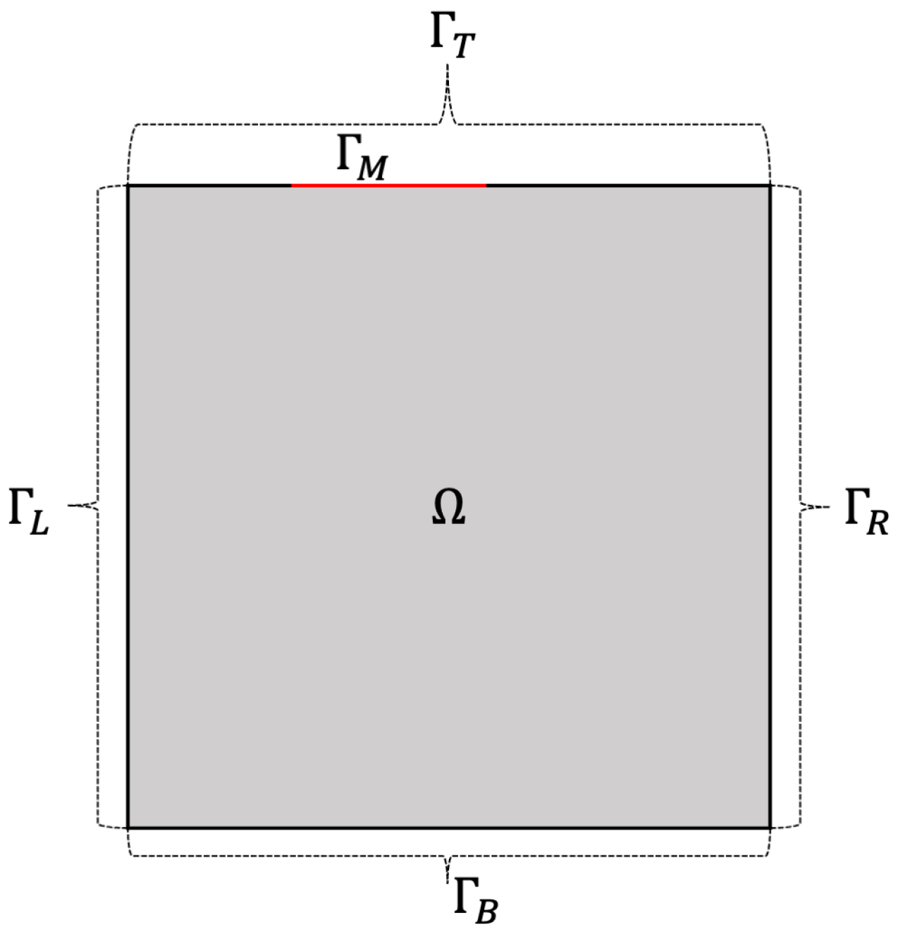
and boundary conditions

$$\begin{array}{cc}\hfill & -k\left(T\right)\nabla T·n=\gamma (T-T_{env}),x\in {\mathrm{\Gamma }}_T,-k\left(T\right)\nabla T·n=0,x\in \partial \mathrm{\Omega }\backslash {\mathrm{\Gamma }}_T,\hfill \\ \hfill & u_1=0,{(\sigma \left(u\right)·n)}_2=0,x\in {\mathrm{\Gamma }}_L\cup {\mathrm{\Gamma }}_R,u_2=0,{(\sigma \left(u\right)·n)}_1=0,x\in {\mathrm{\Gamma }}_B,\hfill \\ \hfill & \sigma \left(u\right)·n={\sigma }_p,x\in {\mathrm{\Gamma }}_M,\sigma \left(u\right)·n=0,x\in {\mathrm{\Gamma }}_T\backslash {\mathrm{\Gamma }}_M,\hfill \end{array}$$

(11)

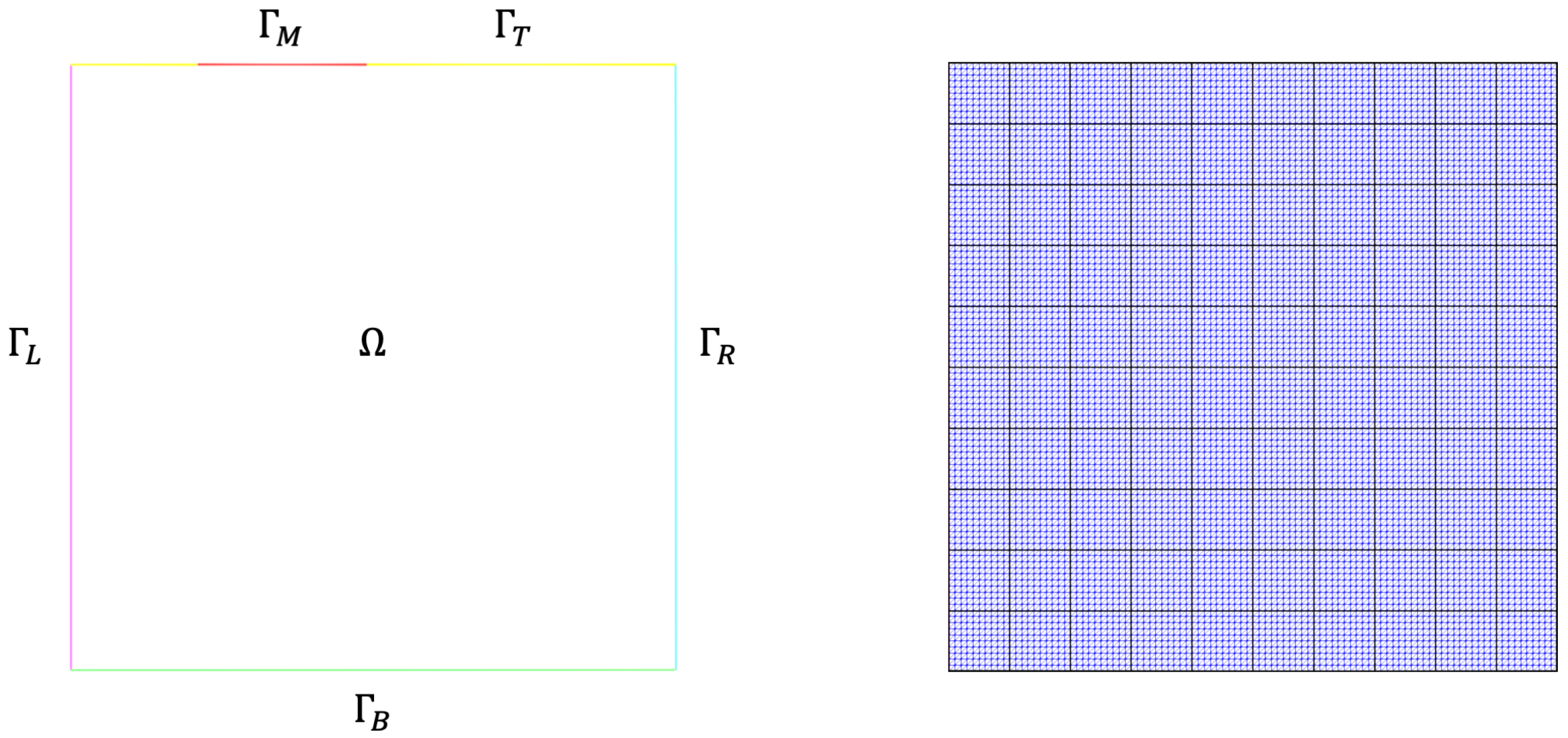
where n is the outward unit normal vector to $\partial \mathrm{\Omega }$; ${\mathrm{\Gamma }}_L$, ${\mathrm{\Gamma }}_R$, ${\mathrm{\Gamma }}_B$, and ${\mathrm{\Gamma }}_T$ denote the left, right, bottom, and top boundaries of $\mathrm{\Omega }$ and ${\mathrm{\Gamma }}_M\subset {\mathrm{\Gamma }}_T$ (see Figure 1); $\sigma \left(u\right)$ is a stress tensor defined as follows:

$$\sigma \left(u\right)=2\mu \left(T\right)\epsilon \left(u\right)+\lambda \left(T\right)\mathrm{tr}\left(\epsilon \left(u\right)\right)\mathcal{I},\epsilon \left(u\right)=\frac{1}{2}(\nabla u+{(\nabla u)}^T).$$

Here, $\epsilon \left(u\right)$ is a deformation tensor and $\mathcal{I}$ is a unit matrix.

Figure 1. Illustration of the computational domain $\mathrm{\Omega }$ with boundaries.

Figure 1. Illustration of the computational domain $\mathrm{\Omega }$ with boundaries.

4. Fine-Grid Approximation

This section presents an approximation of the thermo-mechanical model on a fine grid. The fine-grid solution is accurate and can be considered as the reference one. However, calculations on a fine grid require huge computational resources.

In the section, the variational formulation of the problem is first described. For this purpose, temporal and spatial approximations were performed using a finite difference method and a finite element method, respectively. Then, the discretization on a fine grid and the algorithm for solving the discrete problem are presented.

4.1. Variational Formulation

For performing temporal approximation, the time derivative in the heat equation is replaced with the following finite difference:

$$\frac{\partial T}{\partial t}\approx \frac{T^{n+1}-T^n}{\tau },$$

where $n=0,\dots ,N_t-1$ is a time step number, $N_t$ is a time steps count, $\tau =t_{max}/N_t$ is a time step size. Therefore, our non-stationary problem is transformed into a series of stationary problems.

Next, let $T^{n+1}\in Q$ and $u^{n+1}\in V$ for all time steps, where the function spaces are defined as follows:

$$Q=H^1\left(\mathrm{\Omega }\right),V=\{v\in {\left[H^1\left(\mathrm{\Omega }\right)\right]}^2:v_1\left(x\right)=0,x\in {\mathrm{\Gamma }}_L\cup {\mathrm{\Gamma }}_R\mathrm{and}{v}_2\left(x\right)=0,x\in {\mathrm{\Gamma }}_B\},$$

where $H^1$ is Sobolev space. Then, the heat and mechanics equations are multiplied by arbitrary test functions $q\in Q$ and $v\in V$, respectively. The obtained equations are integrated using the integration by parts formula and considering (11). As a result, the following variational formulation is obtained.

For $n=0,\dots ,N_t-1$, find $T^{n+1}\in Q$ and $u^{n+1}\in V$ such that

$$\begin{array}{cc}\hfill & s(\frac{T^{n+1}-T^n}{\tau },q)+a_T(T^{n+1},q)=l_T\left(q\right),\forall q\in Q,\hfill \\ \hfill & a_u(u^{n+1}-u^n,v)=l_u\left(v\right)+b(T^{n+1}-T^n,v),\forall v\in V,\hfill \end{array}$$

where the bilinear and linear forms are defined as follows:

$$\begin{gathered} s(T,q)={\int }_{\mathrm{\Omega }}\left[{\left(c\rho \right)}^n+{\left(D{w}^{\prime }\right)}^n\right]Tqdx, \\ {a}_T(T,q)={\int }_{\mathrm{\Omega }}{k}^n\nabla T·\nabla qdx+{\int }_{{\mathrm{\Gamma }}_T}\gamma Tqds,l_T\left(q\right)={\int }_{{\mathrm{\Gamma }}_T}\gamma T_{env}qds, \\ {a}_u(u,v)={\int }_{\mathrm{\Omega }}\sigma \left(u\right):\epsilon \left(v\right)dx,l_u\left(v\right)={\int }_{{\mathrm{\Gamma }}_M}{\sigma }_p·vds,b(T,v)={\int }_{\mathrm{\Omega }}\left[\beta \left(T\right)\varphi \left(T\right)\mathcal{I}\right]:\epsilon \left(v\right)dx. \end{gathered}$$

Note that the implicit time scheme is used here. For linearizing the heat equation, its coefficients are taken from the previous time step. Since displacements do not affect the temperature in our model, one can solve the heat and mechanics equations sequentially.

4.2. Discrete Formulation

Next, spatial discretization needs to be performed. First, a fine grid ${\mathcal{T}}^h$ consisting of finite elements $K_j$ is defined. Then, a discretized computational domain ${\mathrm{\Omega }}_h={\bigcup }_{j=1}^{N_c^h}{K}_j$ is introduced, where $N_c^h$ is a count of finite elements. Finite-dimensional function spaces $Q_h\subset Q$ and $V_h\subset V$ are defined on ${\mathrm{\Omega }}_h$. In the discrete formulation, $T^{n+1}\in Q_h$ and $u^{n+1}\in V_h$ are sought for each time step that can be represented as follows:

$$T^{n+1}=\sum _{j=1}^{N_v^h}{T}_{h,j}^{n+1}{\varphi }_j,u^{n+1}=\sum _{j=1}^{2N_v^h}{u}_{h,j}^{n+1}{\mathrm{\Phi }}_j,$$

where ${\varphi }_j$ and ${\mathrm{\Phi }}_j$ are standard linear basis functions, $T_{h,j}^{n+1}$ and $u_{h,j}^{n+1}$ are nodal values vectors of temperature and displacements.

One can write the discrete problem in a matrix-vector form as follows. For $n=0,\dots ,N_t-1$:

• Find the vector of temperature nodal values $T_h^{n+1}$ such that

  $$S\frac{T_h^{n+1}-T_h^n}{\tau }+A_T{T}_h^{n+1}=L_T,$$

  where the matrices and vectors are as follows:

  $$\begin{array}{c}S=\left[s_{ij}\right],s_{ij}=s({\varphi }_i,{\varphi }_j),\\ A_T=\left[a_{T,ij}\right],a_{T,ij}=a_T({\varphi }_i,{\varphi }_j),L_T=\left\{l_{T,j}\right\},l_{T,j}=l_T\left({\varphi }_j\right).\end{array}$$
• Find the vector of displacements nodal values $u_h^{n+1}$ such that

  $$A_u(u_h^{n+1}-u_h^n)=L_u+B^{n+1}-B^n,$$

  where the matrices and vectors are defined as follows:

  $$\begin{array}{c}{A}_u=\left[a_{u,ij}\right],a_{u,ij}=a_u({\mathrm{\Phi }}_i,{\mathrm{\Phi }}_j),L_u=\left\{l_{u,j}\right\},l_{u,j}=l_u\left({\mathrm{\Phi }}_j\right),\\ B^{n+1}=\left\{b_j^{n+1}\right\},b_j^{n+1}=b(T^{n+1},{\mathrm{\Phi }}_j),B^n=\left\{b_j^n\right\},b_j^n=b(T^n,{\mathrm{\Phi }}_j).\end{array}$$

The resulting heat and mechanics discrete systems have $N_v^h$ and $2N_v^h$ degrees of freedom, respectively. In the next two sections, multiscale strategies that can reduce the sizes of the discrete problems are presented.

5. Offline Coarse-Grid Approximation

This section presents an offline multiscale model reduction technique based on the GMsFEM for the thermo-mechanical model. This multiscale approach can significantly decrease computational costs, but it does not consider the problem’s nonlinearity and can be inaccurate. In the section, a general description of GMsFEM is given. Then, the construction of multiscale basis functions for temperature and displacements is described. Finally, an algorithm for solving the problem on a coarse grid using the computed basis functions is given.

The Generalized Multiscale Finite Element Method (GMsFEM) is a general approach for performing multiscale simulations in complex heterogeneous media. The main idea of the GMsFEM is to construct multiscale basis functions via solving local spectral problems. Such basis functions can handle various fine-scale heterogeneities of the media and allow us to solve problems on a coarse grid. Moreover, one can use more than one basis function per coarse-grid element. This feature is essential for solving complex problems in heterogeneous media with high contrast. The resulting computational macroscopic model has similarities with multicontinuum models since it involves multiple macroscopic parameters.

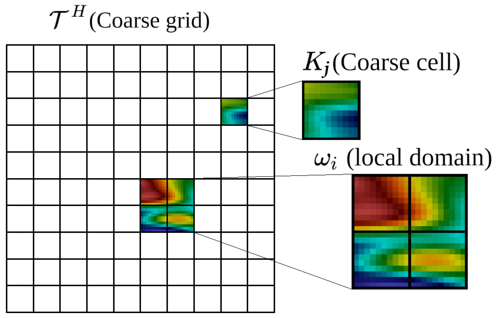
One can divide the algorithm of the GMsFEM into offline and online stages. In the offline stage, our multiscale basis functions that can consider the heterogeneities of the medium are constructed. The basis functions are computed in local domains ${\omega }_i$ of a coarse grid ${\mathcal{T}}^H$. The local domain ${\omega }_i$ consists of coarse-grid cells $K_j$ containing a coarse-grid node $x_i$, i.e., ${\omega }_i=\{K_j\in {\mathcal{T}}^H:x_i\in K_j\}$ (see Figure 2). The offline stage has the following steps.

Offline Stage

• Generate the coarse grid ${\mathcal{T}}^H$.
• For each local domain ${\omega }_i$, compute snapshot functions and construct a snapshot space.
• For each local domain ${\omega }_i$, compute multiscale basis functions via solving local spectral problems on the snapshot space and construct a multiscale space.
• Build a projection matrix into the multiscale space.

Figure 2. Coarse grid ${\mathcal{T}}^H$, coarse cell $K_j$, and local domain ${\omega }_i$.

Figure 2. Coarse grid ${\mathcal{T}}^H$, coarse cell $K_j$, and local domain ${\omega }_i$.

In the online stage, our fine-grid system is projected to the coarse grid using the obtained projection matrix and solves the coarse-grid problem. Note that one can reconstruct the solution on the fine grid. The online stage can be divided into the following steps.

Online Stage

• For the current time step, project the fine-grid system to the coarse grid using the multiscale projection matrix.
• Solve the coarse-grid problem.
• Reconstruct the solution on the fine grid.
• Move to the next time step.

Since the heat and mechanics problems are solved sequentially, multiscale basis functions for temperature and displacements are constructed separately. In the next subsection, the basis functions construction algorithms for both fields are presented. It is supposed that the coarse grid and local domains have been constructed. Therefore, the algorithm starts with the snapshot functions calculation. Note that, wherever possible, the subscript i in the notation of the local domain will be omitted for simplicity of presentation.

5.1. Construction of Multiscale Basis Functions for Temperature

• Snapshot Functions.

To construct snapshot functions for temperature, one needs to solve the following local problems. For each local domain $\omega$, find ${\psi }_j^{\omega }$ such that

$${\int }_{\omega }k\left(T_0\right)\nabla {\psi }_j^{\omega }·\nabla qdx=0,$$

with the following Dirichlet boundary conditions

$${\psi }_j^{\omega }={\delta }_j^h\left(x\right),x\in \partial \omega ,$$

where ${\delta }_j^h\left(x\right)={\delta }_{j,k},\forall j,k\in J_h\left(\omega \right)$, and $J_h\left(\omega \right)$ is a set of all fine-grid nodes on $\partial \omega$. Note that one has to solve $N^{\partial \omega }$ local problems, where $N^{\partial \omega }$ denotes a count of the fine-grid nodes on $\partial \omega$. After that, a snapshot space and a snapshot projection matrix are constructed for each local domain

$$\begin{array}{cc}\hfill & Q_{snap}\left(\omega \right)=span\{{\psi }_j^{\omega }:1\le j\le N^{\partial \omega }\},\hfill \\ \hfill & R_{T,snap}^{\omega }=({\psi }_1^{\omega },\dots ,{\psi }_{N^{\partial \omega }}^{\omega ,snap}).\hfill \end{array}$$

• Multiscale basis functions.

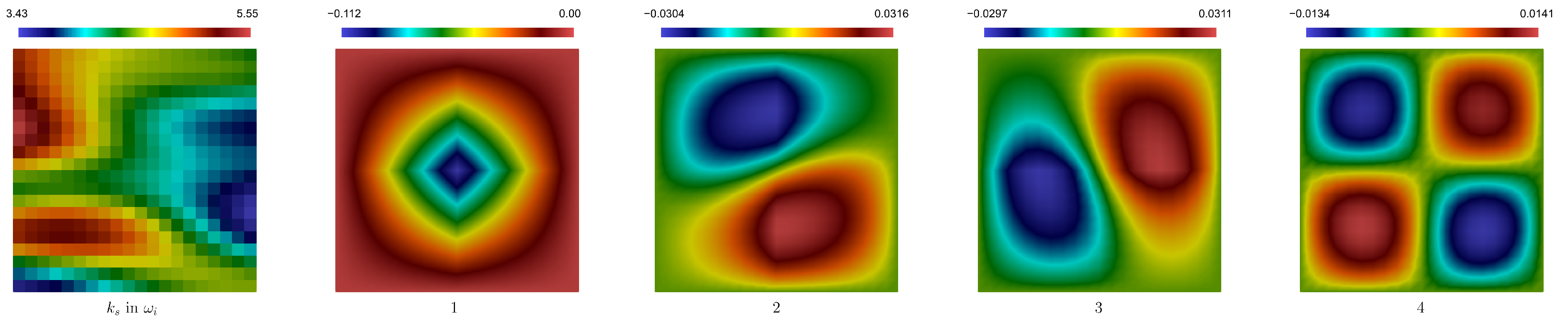
The obtained snapshot projection matrices are used for constructing multiscale basis functions. One needs to solve the following local spectral problems. For each local domain $\omega$, find ${\tilde{\psi }}_k^{\omega }$ such that

$${\tilde{A}}_T{\tilde{\psi }}_k^{\omega }={\lambda }_k{\tilde{S}}_T{\tilde{\psi }}_k^{\omega },$$

where

$$\begin{gathered} {\tilde{A}}_T={\left(R_{T,snap}^{\omega }\right)}^T{A}_T{R}_{T,snap}^{\omega },{\tilde{S}}_T={\left(R_{T,snap}^{\omega }\right)}^T{S}_T{R}_{T,snap}^{\omega }, \\ \begin{array}{c}{A}_T=\left[a_{T,ij}\right],a_{T,ij}={\int }_{\omega }k\left(T_0\right)\nabla {\varphi }_i·\nabla {\varphi }_{j}dx,S_T=\left[s_{T,ij}\right],s_{T,ij}={\int }_{\omega }k\left(T_0\right){\varphi }_i{\varphi }_{j}dx.\end{array} \end{gathered}$$

The resulting eigenvalues are sorted in ascending order and select the eigenvectors corresponding to the first $M_{off}$ eigenvectors. Then, these eigenvectors are projected back to the original space as follows:

$${\overline{\psi }}_k^{\omega }=R_{T,snap}^{\omega }{\tilde{\psi }}_k^{\omega }.$$

To obtain conforming basis functions, the resulting eigenvectors are multiplied by a partition of unity function ${\chi }_i$. This function is linear and continuous in ${\omega }_i$, equal to 1 in $x_i$ and 0 in other coarse-grid nodes.

$${\psi }_{i,k}^{off}={\chi }_i{\overline{\psi }}_k^{{\omega }_i},1\le i\le N_v^H,1\le k\le M_{off},$$

where $N_v^H$ is a count of coarse-grid nodes.

Finally, an offline multiscale space and its projection matrix are constructed as follows:

$$\begin{array}{cc}\hfill & Q_{off}=span\{{\psi }_{i,k}^{off}:1\le i\le N_v^H\mathrm{and}1\le k\le M_{off}\},\hfill \\ \hfill & R_T^{off}=({\psi }_{1,1}^{off},\dots ,{\psi }_{1,M_{off}}^{off},\dots ,{\psi }_{N_v^H,1}^{off},\dots ,{\psi }_{N_v^H,M_{off}}^{off}).\hfill \end{array}$$

Examples of the obtained multiscale basis functions are presented in Figure 3.

5.2. Construction of Multiscale Basis Functions for Displacements

• Snapshot functions.

As for temperature, one needs to solve local problems to obtain snapshot functions. However, the local problems should be solved for each direction of displacements. For each local domain $\omega$ and $l=1,2$, find ${\mathrm{\Psi }}_j^{\omega ,l}$ such that

$${\int }_{\omega }\sigma \left({\mathrm{\Psi }}_j^{\omega ,l}\right):\epsilon \left(v\right)dx=0,$$

with Dirichlet boundary conditions

$${\mathrm{\Psi }}_j^{\omega ,l}={\overline{\delta }}_j^h\left(x\right),x\in \partial \omega ,$$

where ${\overline{\delta }}_j^h\left(x\right)={\delta }_{j,k}{e}_l$, $\forall j,k\in J_h\left({\omega }_i\right)$, $e_l$ is the l-th column of the identity matrix ${\mathcal{I}}_2$. Therefore, one has to solve $2N^{\partial \omega }$ local problems. Then, a snapshot function space and its projection matrix are built for each local domain $\omega$ and direction $l=1,2$ as follows:

$$\begin{array}{cc}\hfill & V_{snap}^l\left(\omega \right)=span\{{\mathrm{\Psi }}_j^{\omega ,l}:1<=j<=N^{\partial \omega }\},\hfill \\ \hfill & R_{u,snap}^{\omega ,l}=({\mathrm{\Psi }}_1^{\omega ,l},\dots ,{\mathrm{\Psi }}_{N^{\partial \omega }}^{\omega ,l}).\hfill \end{array}$$

• Multiscale basis functions.

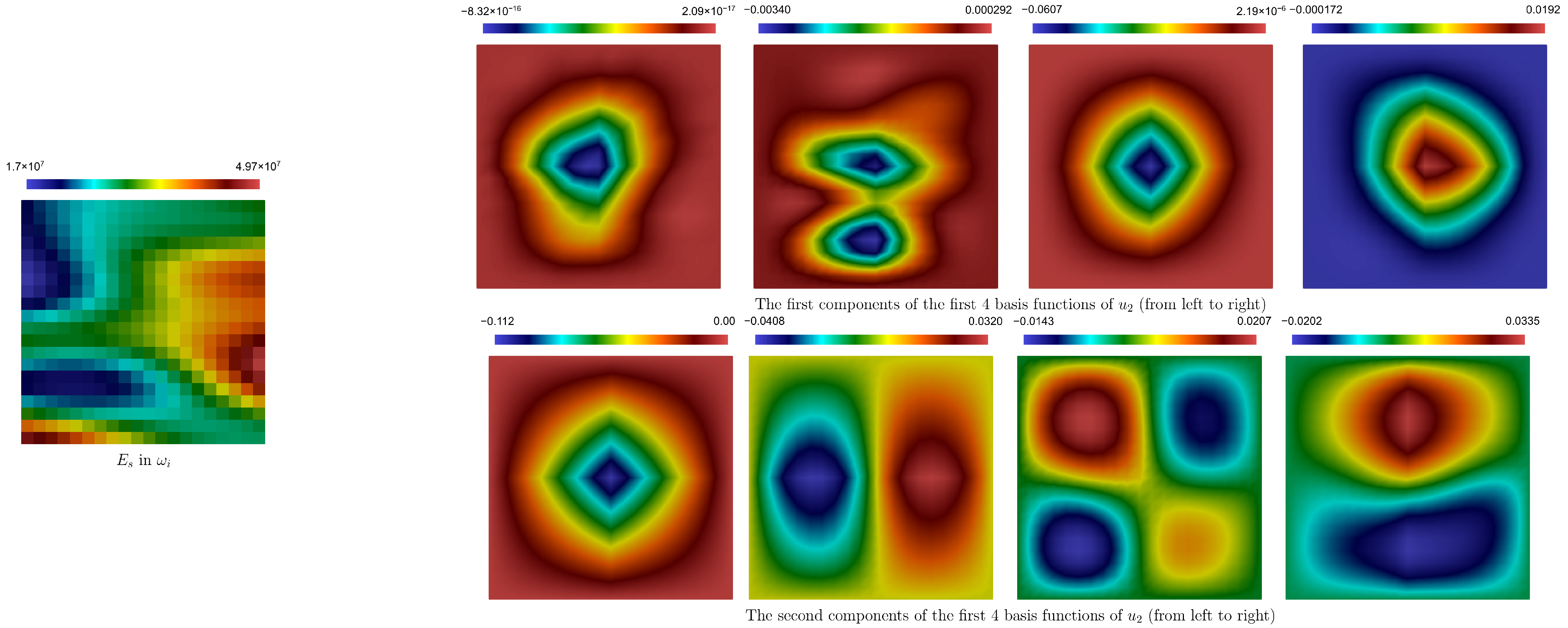
Multiscale basis functions are also constructed separately for each direction of displacements. For this purpose, one needs to solve the following local spectral problems. For each local domain $\omega$ and $l=1,2$, find ${\tilde{\mathrm{\Psi }}}_k^{\omega ,l}$ such that

$${\tilde{A}}_u^l{\tilde{\mathrm{\Psi }}}_k^{\omega ,l}={\lambda }_k^l{\tilde{S}}_u^l{\tilde{\mathrm{\Psi }}}_k^{\omega ,l},$$

where

$$\begin{array}{c}{\tilde{A}}_u^l={\left(R_{u,snap}^{\omega ,l}\right)}^T{A}_u{R}_{u,snap}^{\omega ,l},{\tilde{S}}_u^l={\left(R_{u,snap}^{\omega ,l}\right)}^T{S}_T{R}_{u,snap}^{\omega ,l},\\ A_u=\left\{a_{u,ij}\right\},a_{u,ij}={\int }_{\omega }\sigma \left({\mathrm{\Phi }}_i\right):\epsilon \left({\mathrm{\Phi }}_j\right)dx,\\ S_u=\left\{s_{u,ij}\right\},s_{u,ij}={\int }_{\omega }(\lambda \left(T_0\right)+2\mu \left(T_0\right)){\mathrm{\Phi }}_i·{\mathrm{\Phi }}_{j}dx.\end{array}$$

Next, the resulting eigenvalues are sorted in ascending order and select the eigenvectors corresponding to the first $M_{off}$ eigenvalues. As for temperature, the eigenvectors are projected back using the snapshot projection matrix,

$${\overline{\mathrm{\Psi }}}_k^{\omega ,l}=R_{u,snap}^{\omega ,l}{\tilde{\mathrm{\Psi }}}_k^{\omega ,l}.$$

Then, the resulting eigenvectors are multiplied by the partition of unity function ${\chi }_i$ to obtain conforming basis functions,

$${\mathrm{\Psi }}_{i,k}^{off,l}={\chi }_i{\overline{\mathrm{\Psi }}}_k^{{\omega }_i,l},1\le i\le N_v^H,1\le k\le M_{off},1\le l\le 2.$$

Finally, the multiscale space and its projection matrix are built as follows:

$$\begin{array}{cc}\hfill & V_{off}=span\{{\mathrm{\Psi }}_{i,k}^{off,l}:1\le i\le N_v^H,1\le k\le M_{off},1\le l\le 2\},\hfill \\ \hfill & R_u^{off}=({\mathrm{\Psi }}_{1,1}^{off,1},\dots ,{\mathrm{\Psi }}_{N_v^H,M_{off}}^{off,2}).\hfill \end{array}$$

Figure 4 and Figure 5 present examples of the obtained multiscale basis functions in $x_1$ and $x_2$ directions, respectively.

5.3. Coarse-Grid System

Using the resulting projection matrices for temperature and displacements, one can project the discrete system from a fine grid to a coarse grid. Moreover, the solution can be projected back to the fine grid. Let us take a closer look at all these procedures.

One can write the discrete problems on the coarse grid in the following way. For $n=0,\dots ,N_t-1$,

• Find the vector of temperature nodal values $T_H^{n+1}$ such that

  $$S_H\frac{T_H^{n+1}-T_H^n}{\tau }+A_{T,H}{T}_H^{n+1}=L_{T,H},$$

  where the matrices and vectors are as follows:

  $$\begin{array}{c}{S}_H={\left(R_T^{off}\right)}^{T}S{R}_T^{off},A_{T,H}={\left(R_T^{off}\right)}^T{A}_T{R}_T^{off},\\ L_{T,H}={\left(R_T^{off}\right)}^T{L}_T,T_H^n={\left(R_T^{off}\right)}^T{T}_h^n.\end{array}$$
• Find the vector of displacements nodal values $u_H^{n+1}$ such that

  $$A_{u,H}(u_H^{n+1}-u_H^n)=L_{u,H}+B_H^{n+1}-B_H^n,$$

  where the matrix and vectors are obtained as follows:

  $$\begin{array}{c}{A}_{u,H}={\left(R_u^{off}\right)}^T{A}_u{R}_u^{off},B_H^n={\left(R_u^{off}\right)}^T{B}^n,L_{u,H}={\left(R_u^{off}\right)}^T{L}_u,u_H^n={\left(R_u^{off}\right)}^T{u}_h^n.\end{array}$$

One can reconstruct the fine-grid solutions as follows:

$$T_{off}^{n+1}=R_T^{off}{T}_H^{n+1},u_{off}^{n+1}=R_u^{off}{u}_H^{n+1}.$$

As mentioned before, this multiscale model reduction approach does not consider the nonlinearity caused by phase change. For this purpose, an online enrichment technique will be considered in the next section.

6. Online Enrichment of Offline Coarse-Grid Approximation

The thermo-mechanical model with phase change is nonlinear because the coefficients depend on temperature. The multiscale method described in the previous section does not account for the coefficient changes, which can be a source of errors. In this section, a residual-driven online multiscale approach is presented that can consider media changes.

The section begins with a general description of the online multiscale approach. Then, the constructions of online multiscale basis functions for temperature and displacements are presented. Finally, an algorithm for solving the problem using the online multiscale approach is given.

The residual-driven online multiscale approach can update information about the medium while solving the problem. For this purpose, it computes additional online multiscale basis functions and enriches the offline space. Since calculating these basis functions for each time step can be expensive, it is preferable to update online basis functions every five to ten time steps. One can also enrich the offline space adaptively for some local domains with a large residual, as described by Chung et al. in [34,38]. The online enrichment algorithm can be outlined as follows:

Online Stage

• Generate the coarse-grid system for the current time step.
• Solve the coarse-grid system.
• Compute online multiscale basis functions, enrich the offline multiscale space, repeatedly solve the problem for the current time step.
• Move to the next time step.

Since temperature and mechanics problems are solved sequentially, their online multiscale basis functions are computed separately.

• Online multiscale basis functions for temperature.

One has to solve the following local problems for calculating online multiscale basis functions for temperature. For each local domain $\omega$, find ${\psi }_k^{\omega }$ such that

$$\begin{array}{cc}\hfill & s(\frac{{\psi }_k^{\omega }}{\tau },q)+a_T({\psi }_k^{\omega },q)=r_T^{k-1}\left(q\right),x\in \omega ,\hfill \\ \hfill & {\psi }_k^{\omega }=0,x\in \partial \omega \backslash {\gamma }_T.\hfill \end{array}$$

Here, ${\gamma }_T=\partial \omega \cap {\mathrm{\Gamma }}_T$, and the residual term $r_T^k\left(q\right)$ is defined as follows:

$$r_T^k\left(q\right)=l_T\left(q\right)+s(\frac{T_{ms}^n}{\tau },q)-s(\frac{T_{ms}^k}{\tau },q)-a_T(T_{ms}^k,q),$$

where the subscript $ms$ denotes the multiscale solution.

Next, the obtained functions are multiplied by the partition of unity functions,

$${\psi }_{i,k}^{on}={\chi }_i{\psi }_k^{{\omega }_i},1\le i\le N_v^H.$$

Finally, the multiscale space is enriched using the obtained online basis functions,

$$Q_{ms}=span\{{\psi }_{i,j}^{off},{\psi }_{i,k}^{on}:1\le i\le N_v^H,1\le j\le M_{off},1\le k\le M_{on}\},$$

where k is the number of online iterations for the current time step.

• Online multiscale basis functions for displacements.

As for temperature, one has to solve the local problems for calculating online multiscale basis functions. For each local domain $\omega$, find ${\mathrm{\Psi }}_k^{\omega }$ such that

$$\begin{array}{cc}\hfill & a_u({\mathrm{\Psi }}_k^{\omega },v)=r_u^{k-1}\left(v\right),x\in \omega ,\hfill \\ \hfill & {\mathrm{\Psi }}_k^{\omega }=0,x\in \partial \omega \backslash {\gamma }_M,\hfill \end{array}$$

where ${\gamma }_M=\partial \omega \cap {\mathrm{\Gamma }}_M$, and the residual term $r_u^k\left(v\right)$ has the following form:

$$r_u^k\left(v\right)=l_u\left(v\right)+b(T_{ms}^{n+1}-T_{ms}^n,v)+a_u(u_{ms}^n,v)-a_u(u_{ms}^k,v).$$

For obtaining conforming basis functions, the resulting functions are multiplied by the partition of unity functions as follows:

$${\mathrm{\Psi }}_{i,k}^{on}={\chi }_i{\mathrm{\Psi }}_k^{{\omega }_i},1\le i\le N_v^H.$$

Next, these basis functions are multiplied by $e_l$ to obtain the online basis functions corresponding to each direction,

$${\mathrm{\Psi }}_{i,k}^{l,on}=e_l{\mathrm{\Psi }}_{i,k}^{on},1\le i\le N_v^H,1\le l\le 2.$$

At the end, the multiscale space is enriched with these online basis functions,

$$V_{ms}=span\{{\mathrm{\Psi }}_{i,j}^{l,off},{\mathrm{\Psi }}_{i,k}^{l,on}:1\le i\le N_v^H,1\le j\le M_{off},1\le k\le M_{on},1\le l\le 2\},$$

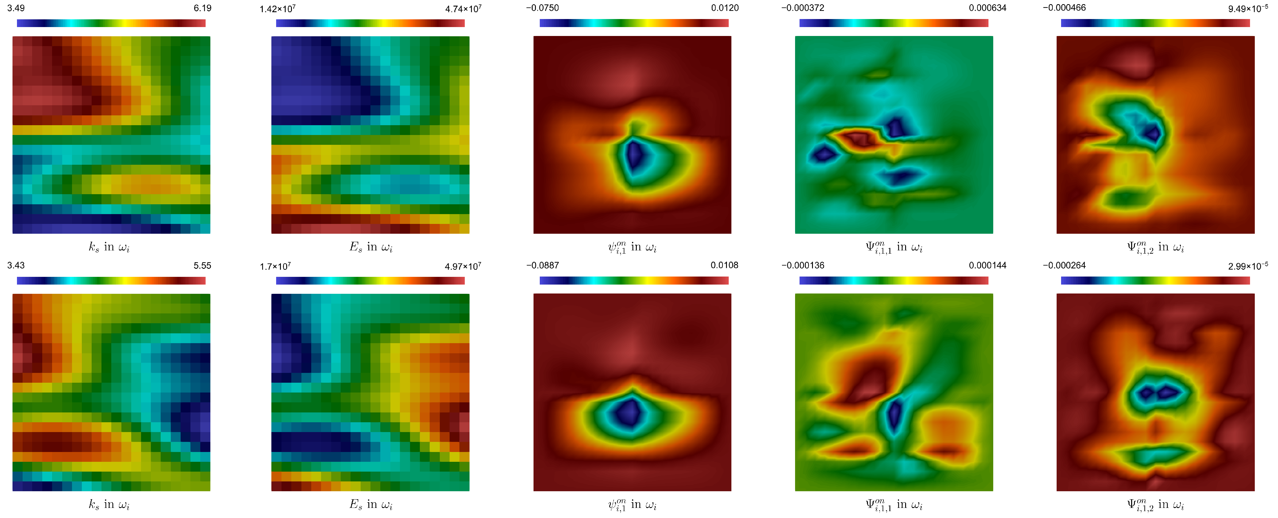
where k is the number of online iterations for the current time step. Examples of the online basis functions for temperature and displacements are depicted in Figure 6. Finally, the detailed algorithm of our multiscale approach with online residual-driven enrichment is presented in the next paragraph.

• Multiscale algorithm with online enrichment.

One can define the following steps of the proposed multiscale algorithm with online residual-driven enrichment. For each time step $n=0,\dots ,N_t-1$,

• Solve the heat problem.

  (a)

  Define the projection matrix $R_T=R_T^n$ for the current time step n, where $R_T=R_T^{off}$ if $n=0$.

  (b)

  Build and solve the coarse-grid system at the current time step.

  i.

  If one wants to add or update online basis functions for the current time step, one needs to solve the following problems. For $k=1,\dots ,M_{on}$, solve

  $$S_H^{k-1}\frac{T_H^k-T_H^n}{\tau }+A_{T,H}^{k-1}{T}_H^k=L_{T,H}^{k-1},$$

  where the matrices and vectors follow

  $$\begin{array}{c}{S}_H^k={\left(R_T^k\right)}^{T}S{R}_T^k,A_{T,H}^k={\left(R_T^k\right)}^T{A}_T{R}_T^k,L_{T,H}^k={\left(R_T^k\right)}^T{L}_T,\\ R_T^k=({\psi }_{1,1}^{off},\dots ,{\psi }_{N_v^H,M_{off}}^{off},{\psi }_{1,1}^{on},\dots ,{\psi }_{N_v^H,k}^{on}).\end{array}$$

  Here, $R_T^k=R_T^{off}$ for $k=0$. The online basis functions ${\psi }_{i,k}^{on}$ are computed using the solution from the previous iteration of k. After all online iterations, one sets $R=R_T^{M_{on}}$.

  ii.

  Solve

  $$S_H\frac{T_H^{n+1}-T_H^n}{\tau }+A_{T,H}{T}_H^{n+1}=L_{T,H},$$

  where

  $$S_H={\left(R_T\right)}^{T}S{R}_T,A_{T,H}={\left(R_T\right)}^T{A}_T{R}_T,L_{T,H}={\left(R_T\right)}^T{L}_T.$$

• Solve the mechanics problem.

  (a)

  Define the projection matrix $R_u=R_u^n$ for the current time step n, where $R_u=R_u^{off}$ if $n=0$.

  (b)

  Build and solve the coarse-grid system at the current time step.

  i.

  If one wants to add or update online basis functions for the current time step, one solves the following problems. For $k=1,\dots ,M_{on}$, solve

  $$A_{u,H}^{k-1}(u_H^k-u_H^n)=L_{u,H}^{k-1}+B_H^{n+1,k-1}-B_H^{n,k-1},$$

  where

  $$\begin{array}{c}{A}_{u,H}^k={\left(R_u^k\right)}^T{A}_u{R}_u^k,B_H^{k,n}={\left(R_u^k\right)}^T{B}^n{R}_u^k,L_{u,H}^k={\left(R_u^k\right)}^T{L}_u,\\ R_u^k=({\mathrm{\Psi }}_{1,1}^{off,1},\dots ,{\mathrm{\Psi }}_{N_v^H,M_{off}}^{off,2},{\mathrm{\Psi }}_{1,1}^{on,1},\dots ,{\mathrm{\Psi }}_{N_v^H,k}^{on,2}),\end{array}$$

  where $R_u^k=R_u^{off}$ for $k=0$. The online basis functions ${\mathrm{\Psi }}_{i,k}^{on}$ are calculated using the solution from the previous iteration of k. After all online iterations, one sets $R=R_u^{M_{on}}$.

  ii.

  Solve

  $$A_{u,H}(u_H^{n+1}-u_H^n)=L_{u,H}+B_H^{n+1}-B_H^n,$$

  where

  $$A_{u,H}={\left(R_u\right)}^T{A}_u{R}_u,B_H^n={\left(R_u\right)}^T{B}^n{R}_u,L_{u,H}={\left(R_u\right)}^T{L}_u.$$

• Move to the next time step.

Next, the numerical results of the proposed multiscale model reduction approaches will be presented.

7. Numerical Results

This section presents numerical results to test the thermo-mechanical model and the proposed multiscale approaches. A two-dimensional model problem simulating the heaving process of heterogeneous soil with a stiff inclusion was considered. First, the numerical solution of the problem on fine and coarse grids was carried out, and the distributions of solutions are given. Then, the relative errors were calculated to check the efficiency of the multiscale approaches. Finally, the relative errors were plotted over time.

The numerical implementation of the fine-grid and multiscale methods was based on the FEniCS computational package [22]. For visualizing the results, the program ParaView was used [39]. The graphical package Matplotlib was used to visualize the error plots [40].

The two-dimensional model problem defined in $\mathrm{\Omega }=[0,6]\times [0,6]{\mathrm{m}}^2$ was considered. As a fine grid, a uniform grid with 10,201 vertices and 20,000 triangular cells was used. The coarse grid consisted of 121 vertices and 100 rectangular cells. Figure 7 depicts the computational domain and grids.

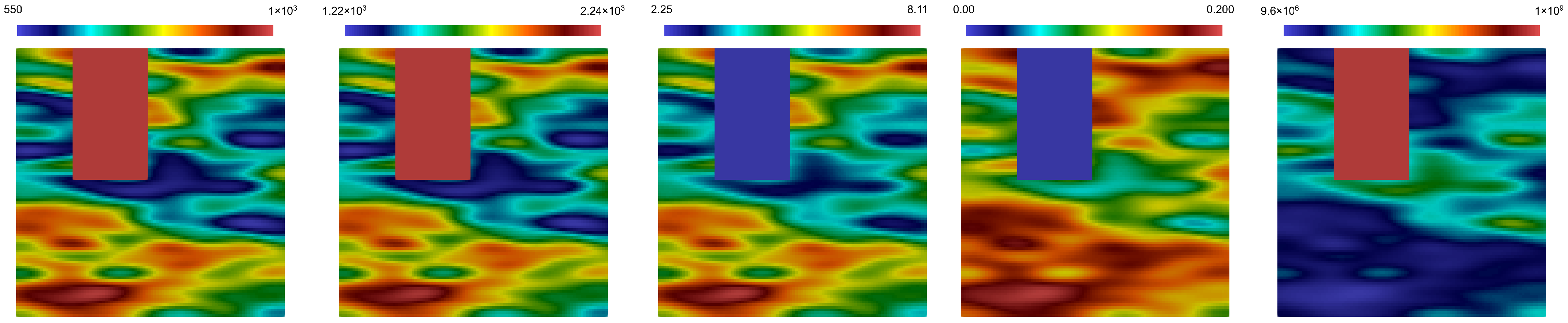
The model problem was simulated for $t_{max}=\mathrm{2,592,000}\mathrm{s}$ with 50 time steps. A heterogeneous soil with a stiff inclusion was considered. For this purpose, the heterogeneous coefficients $c_s$, ${\rho }_s$, $k_s$, $\overline{\varphi }$, and $E_s$ were used (see Figure 8). Poisson’s ratio was set as $\nu =0.3$, and the remaining coefficients were as follows:

• Ice properties:$E_i=9.5·{10}^9\mathrm{Pa}$, $k_i=2.24\mathrm{W}·{\mathrm{m}}^{-1}·{}^{\circ }{\mathrm{C}}^{-1}$, $c_i=2000\mathrm{J}·{\mathrm{kg}}^{-1}·{}^{\circ }{\mathrm{C}}^{-1}$, and ${\rho }_i=917\mathrm{kg}·{\mathrm{m}}^{-3}$.
• Water properties:$k_w=0.56\mathrm{W}·{\mathrm{m}}^{-1}·{}^{\circ }{\mathrm{C}}^{-1}$, $c_w=4180\mathrm{J}·{\mathrm{kg}}^{-1}·{}^{\circ }{\mathrm{C}}^{-1}$, and ${\rho }_w=1000\mathrm{kg}·{\mathrm{m}}^{-3}$.
• Phase change properties:$L=\mathrm{333,000}\mathrm{J}·{\mathrm{kg}}^{-1}$, $T_f=0{}^{\circ }\mathrm{C}$, and $\alpha ={\left(0.3\right)}^{-1}{}^{\circ }{\mathrm{C}}^{-1}$.

Figure 8. Distributions of $c_s$, ${\rho }_s$, $k_s$, $\overline{\varphi }$, and $E_s$.

Figure 8. Distributions of $c_s$, ${\rho }_s$, $k_s$, $\overline{\varphi }$, and $E_s$.

For initial conditions, $T_0=2{}^{\circ }\mathrm{C}$ and $u_0={(0,0)}^T\mathrm{m}$ were set. The boundary conditions (11) were used with $\gamma =14\mathrm{W}·{\mathrm{m}}^{-2}·{}^{\circ }{\mathrm{C}}^{-1}$, $T_{env}=-15{}^{\circ }\mathrm{C}$, and ${\sigma }_p={(0,-{10}^3)}^T\mathrm{Pa}$. The corresponding boundaries of the domain are depicted in Figure 7.

In all the figures of the numerical results, the online multiscale approach results are depicted with an enrichment periodicity equal to five. Figure 9 presents temperature distributions at different points in time. From top to bottom, a fine-grid solution, multiscale solutions using four offline basis functions and using two online and four offline basis functions are depicted, respectively. In the pictures, the white line is the isoline of 0, which corresponds to the phase change temperature. As one can see, all the pictures are very similar, which indicates that our multiscale approaches approximate the fine-grid solution well. However, the isoline of 0 is smoother in the multiscale solution with online enrichment than without it.

In terms of the simulated process, the solutions behave correctly. Initially, the ground is in a thawed state. Then, freezing begins at the top boundary caused by interaction with the low environmental temperature. This leads to a phase change process. One can see that the isoline of 0 becomes lower the longer the freezing takes place. The ground-freezing process is heterogeneous, especially in the area of stiff inclusion.

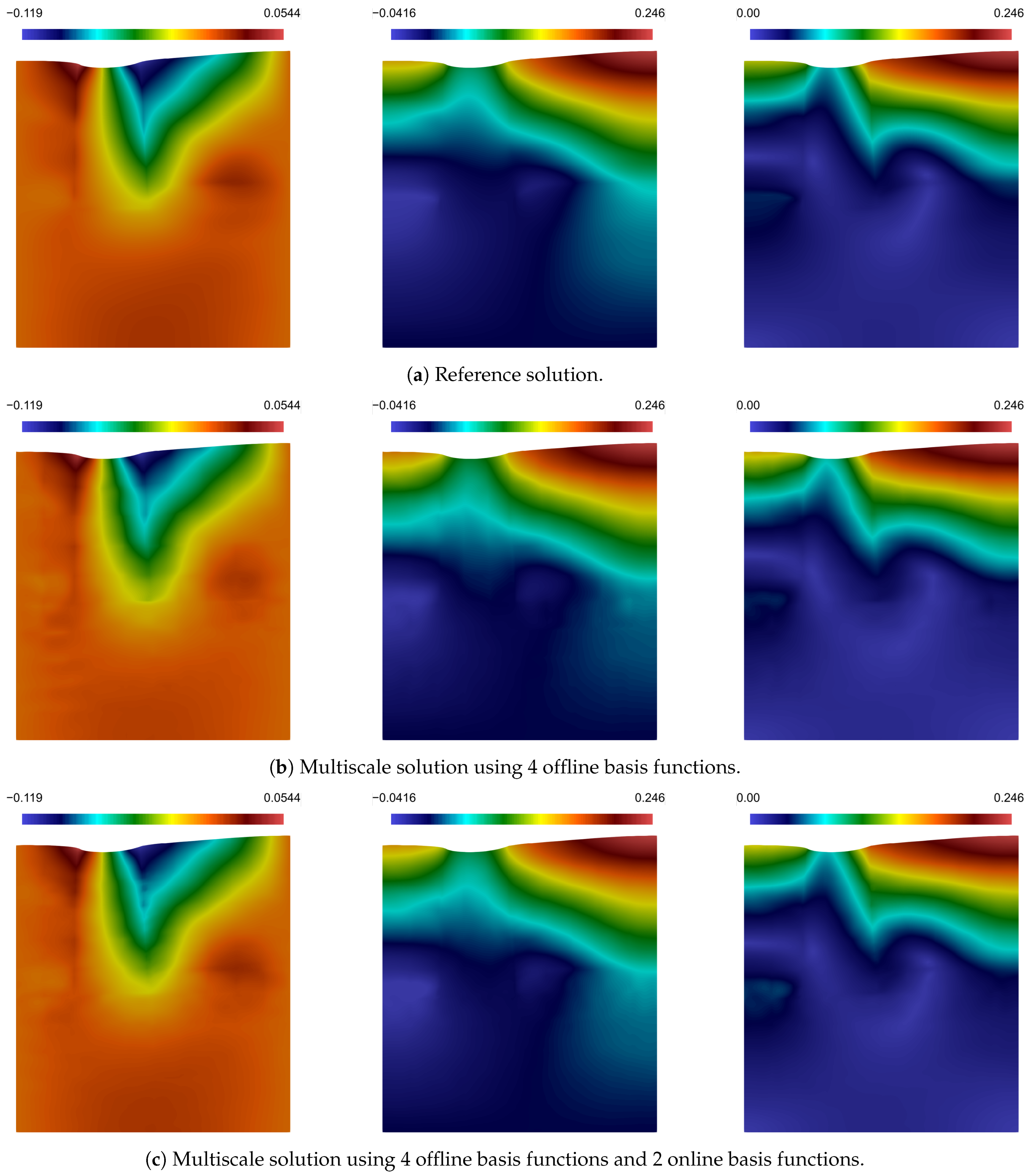
Figure 10 presents distributions of displacements in the $x_1$ and $x_2$ directions and the magnitude of displacements (from left to right) at the last moment. It depicts the fine-grid solution, the multiscale solutions using four offline basis functions and using two online and four offline basis functions (from top to bottom). One can see that all the results are similar to those in the temperature case. However, the differences are more noticeable in the results of the offline multiscale solution.

Note that a warp scale factor of two is used to show the medium’s deformations more clearly. One can observe that the primary displacement occurs in the $x_2$ direction; at the same time, the closer to the top boundary it is, the stronger the displacements are. This phenomenon is explained by the fact that deformations occur due to changes in porosity caused by phase transition. As expected, the displacements in the stiff inclusion region are much smaller than in the rest of the domain. In general, the soil heaving process is displayed correctly.

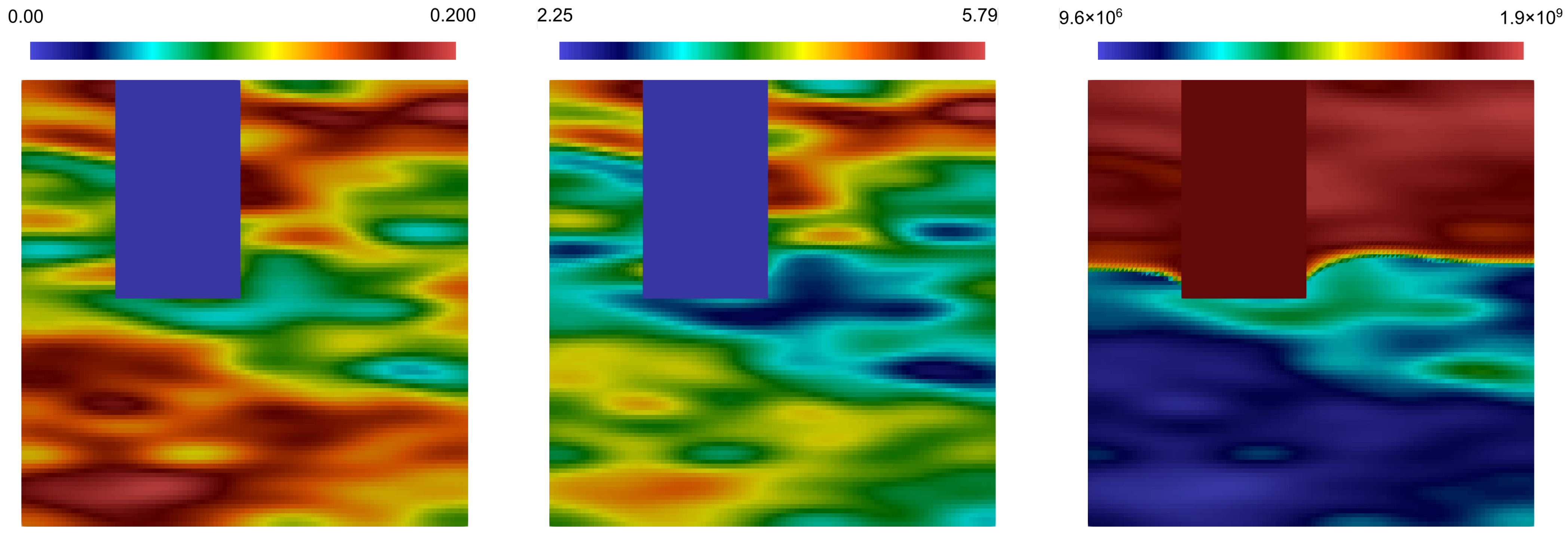
Figure 11 shows the distributions of porosity, heat conductivity, and elastic modulus (from left to right) at the last moment. Only the coefficients of the fine-grid solution are depicted here since the errors of the coefficients of the multiscale solutions are caused by the temperature errors. The distributions of the fine-grid coefficients are presented to observe the influence of phase change on them. One can see that all the coefficients changed because of the phase transition, but the most visible change occurred with the elastic modulus. This phenomenon is because the mechanical properties of ice are very different from those of the soil. Therefore, one can clearly trace the hardening process. Note that the interface of changes in mechanical properties corresponds to the isoline of 0 (see Figure 9).

Next, let us consider the errors of the proposed multiscale approaches. The fine-grid solution was used as the reference one. Two types of error were considered: $L_2$ and energy error. The first shows the error of the solution fields themselves, and the second reflects the error in calculating the gradients. The following formulas were used to calculate the relative $L_2$ errors:

$${ϵ}_{L_2}^T=\sqrt{\frac{{\int }_{\mathrm{\Omega }}{(T-T_{ms})}^{2}dx}{{\int }_{\mathrm{\Omega }}{T}^{2}dx}}\times 100\%,{ϵ}_{L_2}^u=\sqrt{\frac{{\int }_{\mathrm{\Omega }}{(u-u_{ms})}^{2}dx}{{\int }_{\mathrm{\Omega }}{u}^{2}dx}}\times 100\%,$$

and the relative energy errors

$${ϵ}_e^T=\sqrt{\frac{{\int }_{\mathrm{\Omega }}{a}_T(T-T_{ms},T-T_{ms})dx}{{\int }_{\mathrm{\Omega }}{a}_T(T,T)dx}}\times 100\%,{ϵ}_e^u=\sqrt{\frac{{\int }_{\mathrm{\Omega }}{a}_u(u-u_{ms},u-u_{ms})dx}{{\int }_{\mathrm{\Omega }}{a}_u(u,u)dx}}\times 100\%,$$

where the subscript $ms$ corresponds to a multiscale solution (offline or online), and the fields without subscripts denote the fine-grid solutions.

Table 1. Relative errors (%) for temperature and displacements with various numbers of offline and online basis functions (${\mathit{M}}_{off}$ and $M_{on}$). Online basis functions are updated every 5 and 10 time steps (left and right, respectively).

${\mathit{M}}_{\mathit{on}}$	${\mathit{D}\mathit{O}\mathit{F}}_{\mathit{H}}^{\mathit{T}}$	${\mathit{D}\mathit{O}\mathit{F}}_{\mathit{H}}^{\mathit{u}}$	Enrichment Periodicity = 5				Enrichment Periodicity = 10
			${\mathit{ϵ}}_{{\mathit{L}}^{\mathbf{2}}}^{\mathit{T}}$	${\mathit{ϵ}}_{\mathit{e}}^{\mathit{T}}$	${\mathit{ϵ}}_{{\mathit{L}}^{\mathbf{2}}}^{\mathit{u}}$	${\mathit{ϵ}}_{\mathit{e}}^{\mathit{u}}$	${\mathit{ϵ}}_{{\mathit{L}}^{\mathbf{2}}}^{\mathit{T}}$	${\mathit{ϵ}}_{\mathit{e}}^{\mathit{T}}$	${\mathit{ϵ}}_{{\mathit{L}}^{\mathbf{2}}}^{\mathit{u}}$	${\mathit{ϵ}}_{\mathit{e}}^{\mathit{u}}$
			${\mathit{M}}_{\mathit{o}\mathit{f}\mathit{f}}\mathbf{=}\mathbf{1}$				${\mathit{M}}_{\mathit{o}\mathit{f}\mathit{f}}\mathbf{=}\mathbf{1}$
0	121	242	6.785	13.479	30.542	24.562	6.785	13.479	30.542	24.562
1	242	363	3.187	5.93	16.077	19.078	3.681	7.435	19.187	17.908
2	363	484	1.637	2.888	8.324	12.903	2.337	4.338	12.453	14.285
			$M_{off}=2$				$M_{off}=2$
0	242	484	5.317	10.342	25.777	20.197	5.317	10.342	25.777	20.197
1	363	605	2.613	4.698	11.84	15.568	3.108	6.083	16.941	15.459
2	484	726	1.375	2.45	6.824	11.413	2.066	4.003	9.043	11.896
			$M_{off}=4$				$M_{off}=4$
0	484	968	3.577	7.063	11.238	12.775	3.577	7.063	11.238	12.775
1	605	1089	1.499	2.635	5.856	10.561	1.861	3.359	6.038	10.175
2	726	1210	0.812	1.397	3.827	8.555	1.36	2.379	4.901	7.984
			$M_{off}=8$				$M_{off}=8$
0	968	1936	2.02	3.61	5.653	6.945	2.02	3.61	5.653	6.945
1	1089	2057	1.031	1.771	3.399	6.263	1.303	2.228	3.888	6.036
2	1210	2178	0.591	0.969	2.159	5.485	0.973	1.577	2.915	5.166
			$M_{off}=12$				$M_{off}=12$
0	1452	2904	1.427	2.542	4.089	5.147	1.427	2.542	4.089	5.147
1	1573	3025	0.724	1.254	2.349	4.748	0.958	1.623	2.657	4.636
2	1694	3146	0.418	0.699	1.513	4.115	0.72	1.168	2.047	4.078

contains the relative $L_2$ and energy errors at the last moment of time for all fields. The left part corresponds to the update of the online basis functions every five time steps. The right part shows the errors when updating every 10 time steps. The table contains errors for different numbers of offline and online basis functions per coarse-grid node.

Let us consider the results without using online basis functions. One can see that the errors decrease as the number of basis functions increases. Thus, one observes convergence on basis functions. In general, the errors are minor, especially for temperature. For example, when using 12 basis functions, the $L_2$ error is less than $1.5$%, and the energy error is slightly more than $2.5$%; however, the errors of displacements are noticeably larger. For example, for the same number of basis functions, the $L_2$ error is about 4%, and the energy error is more than 5%. This phenomenon is explained by the fact that phase change strongly influences the mechanical properties of the medium.

Next, let us consider the results when using online basis functions updated every five time steps. Adding one or two online basis functions can significantly improve accuracy. For example, if one adds two online basis functions to four offline basis functions, one obtains the following results—the relative $L_2$ error decreases from about $3.6$% to $0.8$% for temperature. At the same time, its relative energy error decreases from about 7% to $1.4$%. For displacements, the $L_2$ error drops from about $11.2$% to $3.8$%, and the energy error decreases from about $12.8$% to $8.6$%. Note that these results are better than when using even eight offline basis functions. Thus, one obtains better accuracy with fewer degrees of freedom.

Then, let us analyze the errors when updating the online basis functions every 10 time steps. As with updating every five time steps, the online basis functions significantly improve the method’s accuracy. The errors are comparable to updating every five time steps, but slightly larger on average. More frequent updates have a noticeable effect with fewer offline basis functions. For example, if one adds two online basis functions to two offline basis functions, one obtains the following results compared to updating once every five time steps—the $L_2$ relativity error in temperature is $2.066$% instead of $1.375$%, and the energy error is $4.003$% instead of $2.45$%. For displacements, one gets the $L_2$ error equal to $9.043$% instead of $6.824$% and the energy error equal to $11.896$% instead of $11.413$%. In general, updating every 10 time steps has comparable errors. This phenomenon can be explained by the fact that the solution does not change significantly quickly in such problems.

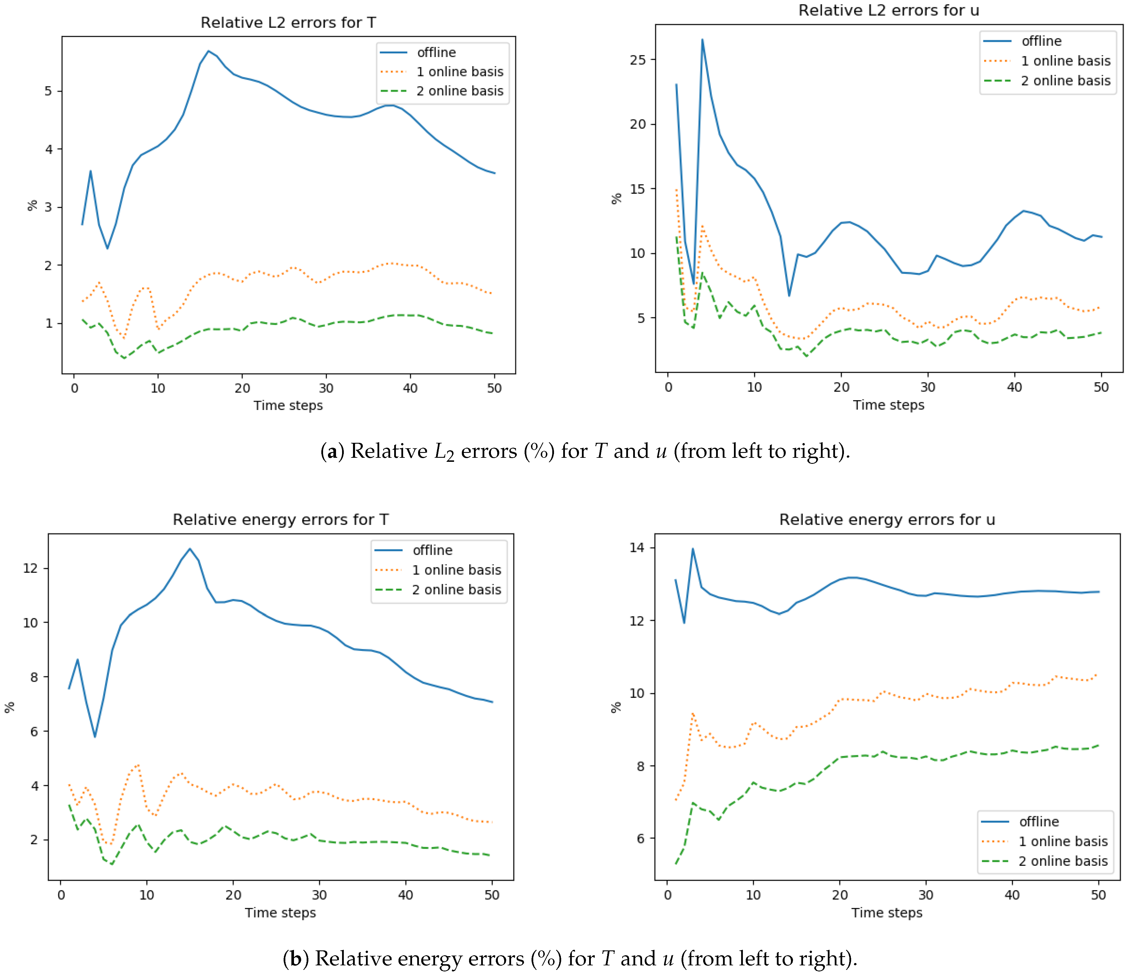
To see the dynamics of the error, the error graphs in time steps were plotted. Figure 12 shows the error dynamics for four offline basis functions with and without online basis functions. The online basis functions are updated every five time steps. Above are the $L_2$ errors, and below are the energy errors. One can see that the errors decrease with each time the online basis functions are updated. In general, the errors fall or remain at about the same level.

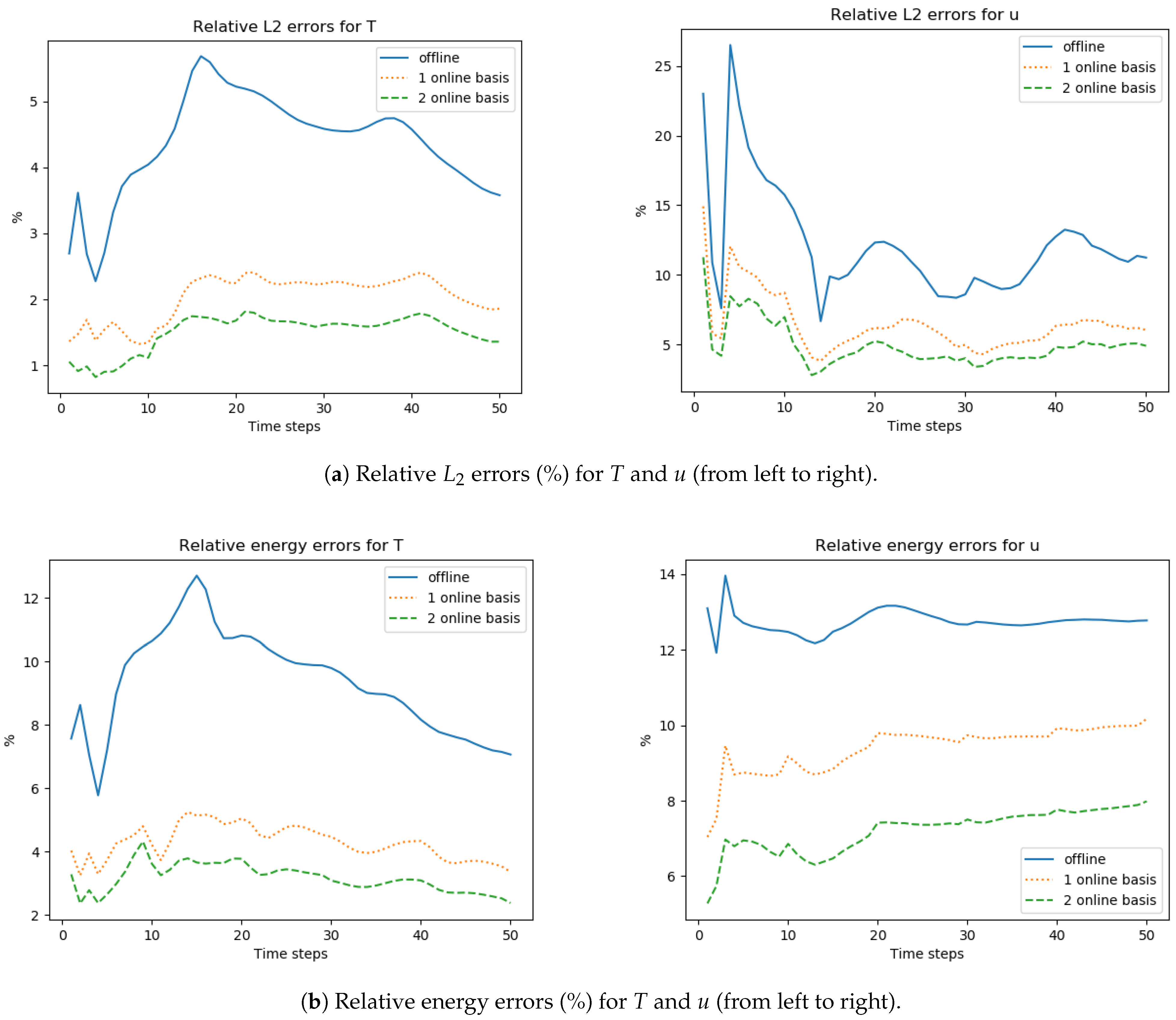
Figure 13 shows the error dynamics when updating the online basis functions every 10 time steps. Above are the $L_2$ errors, and below are the energy errors. As with the update every five time steps, the errors fall with each update of the online basis functions. In general, the errors also either fall or remain at about the same level.

The results show that the online basis functions can significantly improve the accuracy of the multiscale method.

8. Conclusions

In this paper, a thermo-mechanical model with phase transition considering changes in mechanical properties of the medium was presented. For this model, a finite-element approximation on a fine grid was developed. To reduce the size of the discrete problem, multiscale approaches were proposed. An offline multiscale approach based on the Generalized Multiscale Finite Element Method (GMsFEM) was presented. Since the problem is nonlinear, a residual-driven online multiscale approach was also developed.

A two-dimensional model problem of heterogeneous soil heaving with a stiff inclusion was considered. In numerical simulations, the effect of soil heaving caused by the phase transition was observed. Displacements were more substantial the closer they were to the top boundary. However, as expected, the stiff inclusion region displacements were smaller than in the rest of the upper domain. The phase transition interface moved downward as the soil froze. There were changes in the thermal and mechanical properties of the medium corresponding to the phase transition interface. Therefore, the numerical simulation correctly described soil heaving.

Next, offline and online multiscale approaches were considered. In general, both approaches successfully approximated the fine-grid solution with significantly reduced degrees of freedom. The offline multiscale approach can be applied to this problem, but it requires more degrees of freedom for accurate approximation. At the same time, adding online basis functions can significantly improve accuracy with fewer degrees of freedom. Updating online basis functions every five time steps achieved better accuracy than updating every 10 time steps (especially for fewer offline basis functions). However, updating every 10 time steps also provided good accuracy. This phenomenon is because the solution does not change too strongly between time steps. Thus, the online multiscale approach is recommended for the thermo-mechanical model since it provides better accuracy with fewer degrees of freedom.

In terms of applications, the proposed thermo-mechanical model can be used to analyze the stability of structures in permafrost zones. The model problem in the numerical results was motivated by the real-world problems of simulating the behavior of piles during soil frost heaving. Furthermore, the developed online multiscale approach can be used to reduce computational costs when simulating heterogeneous soils.

In future works, more complex mathematical models with phase change, taking into account salinity and filtration, will be considered.