Article

Stability of Impaired Humoral Immunity HIV-1 Models with Active and Latent Cellular Infections

1
Department of Mathematics, Faculty of Science, University of Jeddah, P.O. Box 80327, Jeddah 21589, Saudi Arabia
2
Department of Mathematics, Faculty of Science, King Abdulaziz University, P.O. Box 80203, Jeddah 21589, Saudi Arabia
*
Author to whom correspondence should be addressed.
Computation 2023, 11(10), 207; https://doi.org/10.3390/computation11100207
Submission received: 25 July 2023 / Revised: 2 September 2023 / Accepted: 13 October 2023 / Published: 18 October 2023
(This article belongs to the Special Issue 10th Anniversary of Computation—Computational Biology)

Abstract

:
This research aims to formulate and analyze two mathematical models describing the within-host dynamics of human immunodeficiency virus type-1 (HIV-1) in case of impaired humoral immunity. These models consist of five compartments, including healthy CD4 + T cells, (HIV-1)-latently infected cells, (HIV-1)-actively infected cells, HIV-1 particles, and B-cells. We make the assumption that healthy cells can become infected when exposed to: (i) HIV-1 particles resulting from viral infection (VI), (ii) (HIV-1)-latently infected cells due to latent cellular infection (CI), and (iii) (HIV-1)-actively infected cells due to active CI. In the second model, we introduce distributed time-delays. For each of these systems, we demonstrate the non-negativity and boundedness of the solutions, calculate the basic reproductive number, identify all possible equilibrium states, and establish the global asymptotic stability of these equilibria. We employ the Lyapunov method in combination with LaSalle’s invariance principle to investigate the global stability of these equilibrium points. Theoretical findings are subsequently validated through numerical simulations. Additionally, we explore the impact of B-cell impairment, time-delays, and CI on HIV-1 dynamics. Our results indicate that weakened immunity significantly contributes to disease progression. Furthermore, the presence of time-delays can markedly decrease the basic reproductive number, thereby suppressing HIV-1 replication. Conversely, the existence of latent CI spread increases the basic reproductive number, intensifying the progression of HIV-1. Consequently, neglecting latent CI spread in the HIV-1 dynamics model can lead to an underestimation of the basic reproductive number, potentially resulting in inaccurate or insufficient drug therapies for eradicating HIV-1 from the body. These findings offer valuable insights that can enhance the understanding of HIV-1 dynamics within a host.

1. Introduction

Human immunodeficiency virus type-1 (HIV-1), a retrovirus, targets CD4 + T cells, a pivotal component of the immune system. In a healthy individual, the concentration of CD4 + T cells is typically around 1000 cells/mm 3 . However, following infection, a gradual decline in CD4 + T cell count sets in, and this decrease may persist for years. Whenever the concentration of these cells falls below 200 cells/mm 3 , the individual is diagnosed with Acquired Immune Deficiency Syndrome (AIDS) as indicated by [1]. According to the World Health Organization’s report at the close of 2022, approximately 39 million individuals were living with HIV-1 worldwide [2]. The adaptive immune response has an effective role in resisting and fighting viruses that attack the human body. B-cells and cytotoxic T lymphocytes (CTLs) represent two crucial components of the adaptive immune response. B-cells produce antibodies to counteract HIV-1 particles, while CTLs eliminate cells that have been infected by HIV-1. The assessment of interactions between HIV-1 and both target cells and immune cells can incur significant experimental costs. Consequently, mathematical modeling of HIV-1 infection has become an indispensable tool for comprehending the dynamic behavior of HIV-1 particles and their interactions with target cells and immune cells. The virus dynamics model under the effect of humoral immunity, was introduced in [3] as follows:
Healthy CD 4 + T cells : d F ( t ) d t = ψ Production of healthy cells ρ F t Natural death φ F t K t Infectious transmission ,
( HIV - 1 ) - actively infected cells : d G ( t ) d t = φ F t K t Infectious transmission θ G t Natural death ,
Free HIV - 1 particles : d K ( t ) d t = μ G t Burst size κ K t Natural death σ U ( t ) K ( t ) Neutralization of HIV - 1 ,
B - cells : d U ( t ) d t = ν K ( t ) U ( t ) B - cell stimulation γ U ( t ) Natural death ,
where, F ( t ) , G ( t ) , K ( t ) , and U ( t ) represent the concentrations of healthy CD4 + T cells, (HIV-1)-actively infected cells, free HIV-1 particles, and B-cells at time t. The parameters ψ , φ , μ , σ , and ν correspond to the production rate of healthy CD4 + T cells, incidence (infection) rate, generation rate of HIV-1 from infected cells, neutralization rate of HIV-1 by B-cells, and stimulation rate of the B-cells, respectively. The death rate constants for the four compartments F, G, K, and U are denoted by ρ , θ , κ , and γ , respectively. In this model, it is assumed that HIV-1 particles attack and infect healthy CD4 + T cells. Once the healthy CD4 + T cells become infected, they begin to produce numerous HIV-1 particles. Simultaneously, the B-cells become activated and produce specific antibodies to neutralize the HIV-1 particles. Several extensions were made on this model by involving (i) (HIV-1)-latently infected cells [4], (ii) time-delay [5,6,7], (iii) diffusion [8,9], and (iv) age structure [10,11,12]. The B-cell dynamics can be written as:
d U ( t ) d t = Θ ( K ( t ) , U ( t ) ) γ U ( t ) ,
where Θ ( K , U ) is stimulation of the B-cells. The literature has considered various special forms of Θ ( K , U ) , including:
Form-1. 
One of the special forms of Θ ( K , U ) is the self-regulating humoral response, represented as Θ ( K , U ) = ω , where ω > 0 as discussed in [13].
Form-2. 
Linear humoral response, Θ ( K , U ) = ϕ K , where ϕ > 0 as cited in [14,15,16].
Form-3. 
Another form of Θ ( K , U ) is akin to a predator-prey interaction in the humoral response, expressed as Θ ( K , U ) = ν K U , where ν > 0 as documented in several references including [5,6,7,13,14,15].
Form-4. 
A combination of Form-1, Form-2, and Form-3 for Θ ( K , U ) is represented as Θ ( K , U ) = ω + ϕ K + ν K U , as described in [13].
Form-5. 
The saturated humoral expansion is characterized by Θ ( K , U ) = ν K U ϖ + U , where ϖ > 0 , as discussed in [10,12].
Model (1)–(4) assumes that HIV-1 infection occurs exclusively through viral infection (VI) contact. However, extensive research findings have indicated an alternative route wherein HIV-1 can be directly transmitted from an infected CD4 + T cell to a healthy CD4 + T cell, facilitated by the formation of virological synapses [17,18,19,20,21,22]. This mode of infection, known as cellular infection (CI), exerts a profound impact on HIV-1 transmission, potentially being 100–1000 times more rapid than VI dissemination [23]. Previous investigations have delved into viral infection systems that encompass CI and humoral immunity, with notable studies found in [16,24,25]. In the papers [16,24,25], it was postulated that the presence of antigens solely stimulates the humoral immune response while disregarding any impairment in humoral immunity. According to a report in [26], HIV-1 has the potential to induce impairment in B-cells. When accounting for impaired humoral immunity, the population dynamics of B-cells can be described as shown in various references, including [27,28].
d U ( t ) d t = ϕ K ( t ) γ U ( t ) ε U ( t ) K ( t ) ,
where, ϕ K is stimulation of B-cells and ε U K is the B-cells impairment and ϕ and ε are constants.
In [27,28], the CI was not considered. Recently, Elaiw and Alshehaiween [29] and Elaiw et al. [30] introduced and analyzed virus dynamics models with impaired humoral immunity and CI. The models presented in [29,30] did not take into account the presence of (HIV-1)-latently infected cells. However, Miao et al. in [31] introduced viral infection models that incorporated humoral immunity, (HIV-1)-latently infected cells, and CI. Additionally, in the studies [32,33], the global stability of viral models was investigated, considering factors such as CI, multi-stages of infected cells, and adaptive immunity. In the works [31,32,33], it was assumed that CI solely resulted from the activities of (HIV-1)-actively infected cells. However, it was reported in [34] that (HIV-1)-latently infected cells can also participate in infecting healthy CD4 + T cells through the CI mechanism. Furthermore, in papers such as [35,36,37,38], various virus dynamics models were developed with the consideration that both (HIV-1)-latently and (HIV-1)-actively infected cells contribute to the CI mechanism. However, it’s important to note that these papers did not account for humoral immune impairment.
The objective of this study is to introduce two within-host HIV-1 models that incorporate (HIV-1)-latently infected cells, humoral immune impairment, and the mechanism of CI. In these models, both (HIV-1)-latently infected and (HIV-1)-actively infected cells are considered contributors to CI. The second model further extends the analysis by incorporating three types of distributed time-delays. We perform a comprehensive analysis of both models, including establishing non-negativity and boundedness of solutions, calculating the basic reproductive number, identifying equilibria, assessing global stability, conducting numerical simulations, and engaging in a detailed discussion of the obtained results.

2. Model Incorporating Impaired Humoral Immunity and CI

2.1. Description of the System

We introduce an HIV-1 model that incorporates impaired humoral immunity, considering the infection of healthy CD4 + T cells upon contact with HIV-1 particles, (HIV-1)-latently infected cells, or (HIV-1)-actively infected cells. The model is presented as follows:
d F ( t ) d t = ψ ρ F ( t ) φ 1 F ( t ) K ( t ) φ 2 F ( t ) Q ( t ) φ 3 F ( t ) G ( t ) , d Q ( t ) d t = φ 1 F ( t ) K ( t ) + φ 2 F ( t ) Q ( t ) + φ 3 F ( t ) G ( t ) ( ξ + ϑ ) Q ( t ) , d G ( t ) d t = ξ Q ( t ) θ G ( t ) , d K ( t ) d t = μ G ( t ) κ K ( t ) σ U ( t ) K ( t ) , d U ( t ) d t = ϕ K ( t ) γ U ( t ) ε U ( t ) K ( t ) ,
where Q ( t ) , denotes the concentration of (HIV-1)-latently infected cells at time t. (HIV-1)-latently infected cells are activated at rate ξ Q and die at rate ϑ Q . In this context, φ 1 F K , φ 2 F Q , and φ 3 F G represent the infection rates via HIV-1 particles (VI), (HIV-1)-latently infected cells (CI), and (HIV-1)-actively infected cells (CI), respectively. It is important to note that all these parameters are positive.

2.2. Main Basic Properties

2.2.1. Maintaining Non-Negativity and Boundedness in the Solutions

Lemma 1.
Consider the system (5), there exist positive constants τ i > 0 , i = 1 , 2 , 3 , such that the set
Ω = F , Q , G , K , U R 0 5 : 0 F t , Q t , G t τ 1 , 0 K t τ 2 , 0 U t τ 3
is positively invariant.
Proof. 
To address the nonnegativity of solutions, from system (5) we have
d F d t F = 0 = ψ > 0 , d Q d t Q = 0 = φ 1 F K + φ 3 F G 0 , for all F , K , G 0 , d G d t G = 0 = ξ Q 0 , for all Q 0 , d K d t K = 0 = μ G 0 , for all G 0 , d U d t U = 0 = ϕ K 0 , for all K 0 .
Hence, ( F ( t ) , Q ( t ) , G ( t ) , K ( t ) , U ( t ) ) R 0 5 , for all t 0 when ( F ( 0 ) , Q ( 0 ) , G ( 0 ) , K ( 0 ) , U ( 0 ) ) R 0 5 . Let
Υ t = F t + Q t + G t + θ 2 μ K t + θ κ 4 μ ϕ U t .
Then, we have
d Υ ( t ) d t = d F ( t ) d t + d Q ( t ) d t + d G ( t ) d t + θ 2 μ d K ( t ) d t + θ κ 4 μ ϕ d U ( t ) d t = ψ ρ F t ϑ Q t θ 2 G t θ κ 4 μ K t θ σ 2 μ + θ κ ε 4 μ ϕ U t K t θ κ γ 4 μ ϕ U t ψ ρ F t ϑ Q t θ 2 G t θ κ 4 μ K t θ κ γ 4 μ ϕ U t ψ η F t + Q t + G t + θ 2 μ K t + θ κ 4 μ ϕ U t = ψ η Υ t ,
where η = min ρ , ϑ , θ 2 , κ 2 , γ . Hence,
Υ t e η t Υ 0 ψ η + ψ η .
This yields 0 Υ t τ 1 if Υ 0 τ 1 , where τ 1 = ψ η .
Given that all state variables are non-negative, 0 F t , Q t , G t τ 1 , 0 K t τ 2 , and 0 U t τ 3 , for all t 0 if F 0 + Q 0 + G 0 + θ 2 μ K 0 + θ κ 4 μ ϕ U 0 τ 1 , where τ 2 = 2 μ τ 1 θ and τ 3 = 4 μ ϕ τ 1 θ κ . Hence, F ( t ) , Q ( t ) , G ( t ) , K ( t ) , and U ( t ) are all bounded, indicating that Ω is a positively invariant and compact set with respect to the system (5). □

2.2.2. Analysis of Reproductive Numbers and Equilibrium Points

Lemma 2.
There exists a basic reproductive number 0 = F 0 φ 1 μ ξ + φ 2 κ θ + φ 3 ξ κ ξ + ϑ κ θ for system (5), such that
(i) 
the system always has an infection-free equilibrium point Ξ Q 0 , and
(ii) 
if 0 > 1 , the system also has an infected equilibrium point Ξ Q 1 .
Proof. 
It is evident that system (5) invariably possesses an infection-free equilibrium denoted as Ξ Q 0 = ( F 0 , 0 , 0 , 0 , 0 ) , where F 0 = ψ ρ . In the subsequent analysis, we will employ the next-generation matrix method proposed by Driessche and Watmough [39] to compute the basic reproductive number for system (5). Considering the infected compartments in model (5), arranged as Q , G , K , the nonlinear terms involving the new infection Γ ^ 1 and the outflow term Δ ^ 1 are represented by the following matrices:
Γ ^ 1 = φ 1 F K + φ 2 F Q + φ 3 F G 0 0 ,   Δ ^ 1 = ( ξ + ϑ ) Q ξ Q + θ G μ G + κ K + σ U K .
We calculate the derivatives of Γ ^ 1 and Δ ^ 1 at the equilibrium Ξ Q 0 , resulting in the following matrices:
Γ 1 = φ 2 F 0 φ 3 F 0 φ 1 F 0 0 0 0 0 0 0 ,   Δ 1 = ξ + ϑ 0 0 ξ θ 0 0 μ κ .
The next-generation matrix takes the following form:
Γ 1 Δ 1 1 = F 0 φ 1 μ ξ + φ 2 κ θ + φ 3 ξ κ ξ + ϑ κ θ F 0 φ 1 μ + φ 3 κ κ θ φ 1 F 0 κ 0 0 0 0 0 0 .
The basic reproductive number 0 is defined as the spectral radius of the matrix Γ 1 Δ 1 1 and is calculated as follows:
0 = F 0 φ 1 μ ξ + φ 2 κ θ + φ 3 ξ κ ξ + ϑ κ θ = 01 + 02 + 03 ,
where
01 = F 0 μ ξ φ 1 κ θ ξ + ϑ , 02 = F 0 φ 2 ξ + ϑ , 03 = F 0 ξ φ 3 θ ξ + ϑ .
The parameter 0 holds significant clinical relevance, as it determines whether the HIV-1 infection will become chronic or not. In this context, 01 , 02 , and 03 represent the average numbers of secondary infected cells resulting from contacts with HIV-1 particles, latently infected cells, and actively infected cells, respectively. To identify additional equilibria apart from Ξ Q 0 , we consider F , Q , G , K , U as any equilibrium satisfying the following algebraic equations:
ψ ρ F φ 1 F K φ 2 F Q φ 3 F G = 0 ,
φ 1 F K + φ 2 F Q + φ 3 F G ξ + ϑ Q = 0 ,
ξ Q θ G = 0 ,
μ G κ K σ U K = 0 ,
ϕ K γ U ε U K = 0 .
From Equations (9) and (11), we get
Q = θ G ξ , U = ϕ K γ + ε K .
Upon substitution of Equation (12) into Equation (10), the result is as follows:
G = γ κ K + σ ϕ + κ ε K 2 μ γ + ε K .
Upon substitution of Equation (13) into Equation (12), the result is as follows:
Q = θ γ κ K + σ ϕ + κ ε K 2 ξ μ γ + ε K .
From Equations (7) and (8), we get
ψ ρ F = ξ + ϑ Q .
Upon substitution of Equation (14) into Equation (15), the result is as follows:
F = 1 ρ ψ θ ξ + ϑ γ κ K + σ ϕ + κ ε K 2 ξ μ γ + ε K .
Upon substitution of Equations (13), (14) and (16) into Equation (8), the result is as follows:
K ρ μ 2 ξ 2 γ + ε K 2 A K 3 + B K 2 + C K + D = 0 ,
where
A = θ ξ + ϑ σ ϕ + ε κ ε ξ μ φ 1 + σ ϕ + ε κ θ φ 2 + ξ φ 3 , B = μ ξ φ 1 γ θ ξ + ϑ σ ϕ + 2 ε κ ψ μ ξ ε 2 + σ ϕ + ε κ ε μ ρ ξ θ ξ + ϑ ψ ε μ ξ 2 γ κ θ ξ + ϑ θ φ 2 + ξ φ 3 , C = γ ρ μ ξ θ ξ + ϑ σ ϕ + 2 ε κ + μ ξ φ 1 γ κ θ ξ + ϑ 2 ψ ε μ ξ ψ μ ξ σ ϕ + 2 ε κ γ θ κ 2 ξ + ϑ θ φ 2 + ξ φ 3 , D = μ ρ κ ξ θ γ 2 ξ + ϑ 1 0 ,
where 0 is given by Equation (6). From Equation (17), we have
1
If K = 0 , then from Equations (12)–(14) and (16) the infection-free equilibrium Ξ Q 0 is obtained.
2
If K 0 , we have the equation A K 3 + B K 2 + C K + D = 0 . In this scenario, let us introduce a function Ψ K defined on the interval [ 0 , ) as:
Ψ K = A K 3 + B K 2 + C K + D .
Then
Ψ 0 = μ ρ κ ξ θ γ 2 ξ + ϑ 1 0 < 0 , if 0 > 1 , lim K Ψ K = .
As a result, the function Ψ possesses a positive real root denoted as K 1 . Consequently, by substituting Equations (13) and (14) into Equation (7), we obtain:
F 1 = ψ ρ + φ 1 K 1 + φ 2 Q 1 + φ 3 G 1 ,
where
Q 1 = θ γ κ K 1 + σ ϕ + κ ε K 1 2 ξ μ γ + ε K 1 , G 1 = γ κ K 1 + σ ϕ + κ ε K 1 2 μ γ + ε K 1 , U 1 = ϕ K 1 γ + ε K 1 .
The existence of the infected equilibrium Ξ Q 1 = F 1 , Q 1 , G 1 , K 1 , U 1 is evident when 0 > 1 . □

2.2.3. The Analysis of the Stability of the Equilibria Ξ Q 0 and Ξ Q 1

Theorem 1.
If 0 < 1 , then the equilibrium Ξ Q 0 of system (5) is locally asymptotically stable (L.A.S), and it becomes unstable when 0 > 1 .
Proof. 
In accordance with the study proposed by Willems [40], the local asymptotic stability of the equilibrium Ξ Q 0 can be ascertained by examining the eigenvalues of its associated Jacobian matrix, which is presented as follows:
J = ρ φ 1 K φ 2 Q φ 3 G φ 2 F φ 3 F φ 1 F 0 φ 1 K + φ 2 Q + φ 3 G φ 2 F ϑ + ξ φ 3 F φ 1 F 0 0 ξ θ 0 0 0 0 μ κ + σ U σ K 0 0 0 ϕ ε U γ + ε K .
At the infection-free equilibrium point Ξ Q 0 the Jacobian matrix becomes
J Ξ Q 0 = ρ φ 2 F 0 φ 3 F 0 φ 1 F 0 0 0 φ 2 F 0 ϑ + ξ φ 3 F 0 φ 1 F 0 0 0 ξ θ 0 0 0 0 μ κ 0 0 0 0 ϕ γ .
For matrix (19), the characteristic equation J Ξ Q 0 x I 5 = 0 is solved as x + γ x + ρ Y x = 0 , where x is the eigenvalue, I 5 is the identity matrix and
Y x = x 3 + m 2 x 2 + m 1 x + m 0 ,
and
m 0 = κ θ ξ + ϑ 1 0 > 0 , m 1 = κ θ + κ ξ + ϑ 1 02 + θ ξ + ϑ 1 02 + 03 > 0 , m 2 = κ + θ + ξ + ϑ 1 02 > 0 , m 1 m 2 m 0 = ψ μ ξ φ 1 ρ + θ + ξ + ϑ 1 02 κ ( κ + θ ) + κ ξ + ϑ 1 02 + θ ξ + ϑ 1 02 + 03 > 0 ,
where 0 < 1 .
The Jacobian matrix J Ξ Q 0 is evidently characterized by two negative eigenvalues, γ and ρ . The remaining eigenvalues are determined as the solutions to the cubic equation presented in (20). Applying the Routh-Hurwitz criteria [40], it is apparent that all roots of Equation (20) possess negative real parts. Consequently, the infection-free equilibrium Ξ Q 0 is locally asymptotically stable (L.A.S) when 0 < 1 . Conversely, if 0 > 1 , we have m 0 < 0 , implying that Equation (20) must have at least one positive real root. Hence, the equilibrium Ξ Q 0 becomes unstable when 0 > 1 . □
In the upcoming theorems, we will delve into the global stability of the equilibria. The construction of Lyapunov function is formulated following the method demonstrated in [41]. We defined H z = z 1 ln z and denote F , Q , G , K , U = F t , Q t , G t , K t , U t .
Theorem 2.
For system (5), if 0 < 1 , then Ξ Q 0 is globally asymptotically stable (G.A.S).
Proof. 
Let’s consider a candidate Lyapunov function
Θ 0 = F 0 H F F 0 + Q + ξ + ϑ 1 02 ξ G + θ ξ + ϑ 1 02 + 03 ξ μ K + θ κ ξ + ϑ 1 0 ϕ ξ μ U .
Clearly, Θ 0 ( F , Q , G , K , U ) > 0 for all F , Q , G , K , U > 0 , and Θ 0 ( F 0 , 0 , 0 , 0 , 0 ) = 0 . Computing d Θ 0 d t along with the solutions of model (5), we get
d Θ 0 d t = 1 F 0 F d F d t + d Q d t + ξ + ϑ 1 02 ξ d G d t + θ ξ + ϑ 1 02 + 03 ξ μ d K d t + θ κ ξ + ϑ 1 0 ϕ ξ μ d U d t = 1 F 0 F ψ ρ F φ 1 F K φ 2 F Q φ 3 F G + φ 1 F K + φ 2 F Q + φ 3 F G ξ + ϑ Q + ξ + ϑ 1 02 ξ ξ Q θ G + θ ξ + ϑ 1 02 + 03 ξ μ μ G κ K σ U K + θ κ ξ + ϑ 1 0 ϕ ξ μ ϕ K γ U ε U K = 1 F 0 F ψ ρ F + φ 2 F 0 ξ + ϑ + ξ + ϑ 1 02 Q + φ 3 F 0 θ ξ + ϑ 1 02 ξ + θ ξ + ϑ 1 02 + 03 ξ G + φ 1 F 0 θ κ ξ + ϑ 1 02 + 03 ξ μ + θ κ ξ + ϑ 1 0 ξ μ K γ θ κ ξ + ϑ 1 0 ϕ ξ μ U θ ξ + ϑ ϕ ξ μ ϕ σ 1 02 + 03 + ε κ 1 0 U K .
After performing a direct calculation and utilizing the value F 0 = ψ / ρ , we acquire:
d Θ 0 d t = 1 F 0 F ρ F 0 ρ F γ θ κ ξ + ϑ 1 0 ϕ ξ μ U θ ξ + ϑ ϕ ξ μ ϕ σ 1 02 + 03 + ε κ 1 0 U K = ρ F F 0 2 F γ θ κ ξ + ϑ 1 0 ϕ ξ μ U θ ξ + ϑ ϕ ξ μ ϕ σ 1 02 + 03 + ε κ 1 0 U K .
Clearly, d Θ 0 d t 0 when 0 < 1 and d Θ 0 d t = 0 when F = F 0 and K = U = 0 . Let Φ 0 = F , Q , G , K , U : d Θ 0 d t = 0 , and considering the largest invariant subset of Φ 0 as Φ 0 . Hence, all solutions converge to: Φ 0 [42]. In Φ 0 , all elements satisfy F ( t ) = F 0 and K ( t ) = U ( t ) = 0 . Subsequently, the fourth equation in system (5) yields
0 = d K t d t = μ G t G t = 0 , for all t .
Furthermore, the first equation in system (5) results in
0 = d F ( t ) d t = ψ ρ F 0 φ 2 F 0 Q t Q t = 0 , for all t .
Therefore, Φ 0 = F , Q , G , K , U Φ 0 : F = F 0 , Q = G = K = U = 0 = Ξ Q 0 . Hence, we conclude that Ξ Q 0 is G.A.S whenever 0 < 1 based on LaSalle’s invariance principle (L.I.P) [42]. □
Theorem 3.
If 0 > 1 , the equilibrium Ξ Q 1 of the system (5) is G.A.S.
Proof. 
We consider the function Θ 1 F , Q , G , K , U given by Equation (21) as:
Θ 1 = F 1 H F F 1 + Q 1 H Q Q 1 + F 1 φ 1 μ + φ 3 κ + σ U 1 G 1 θ κ + σ U 1 H G G 1 + φ 1 F 1 K 1 κ + σ U 1 H K K 1 + σ φ 1 F 1 2 κ + σ U 1 ϕ ε U 1 U U 1 2 .
Equilibrium condition Equation (11) guarantees that ϕ ε U 1 = γ U 1 K 1 > 0 . Clearly, Θ 1 is positive definite. Calculating d Θ 1 d t :
d Θ 1 d t = 1 F 1 F d F d t + 1 Q 1 Q d Q d t + F 1 φ 1 μ + φ 3 κ + σ U 1 θ κ + σ U 1 1 G 1 G d G d t + φ 1 F 1 κ + σ U 1 1 K 1 K d K d t + σ φ 1 F 1 κ + σ U 1 ϕ ε U 1 U U 1 d U d t = 1 F 1 F ψ ρ F φ 1 F K φ 2 F Q φ 3 F G + 1 Q 1 Q φ 1 F K + φ 2 F Q + φ 3 F G ξ + ϑ Q + F 1 φ 1 μ + φ 3 κ + σ U 1 θ κ + σ U 1 1 G 1 G ξ Q θ G + φ 1 F 1 κ + σ U 1 1 K 1 K μ G κ K σ U K + σ φ 1 F 1 κ + σ U 1 ϕ ε U 1 U U 1 ϕ K γ U ε U K = 1 F 1 F ψ ρ F + φ 2 F 1 ξ + ϑ + ξ F 1 φ 1 μ + φ 3 κ + σ U 1 θ κ + σ U 1 Q + φ 1 F 1 K + φ 3 F 1 F 1 φ 1 μ + φ 3 κ + σ U 1 κ + σ U 1 + μ φ 1 F 1 κ + σ U 1 G φ 1 F K + φ 2 F Q + φ 3 F G Q 1 Q + ξ + ϑ Q 1 ξ F 1 φ 1 μ + φ 3 κ + σ U 1 θ κ + σ U 1 Q G 1 G + F 1 φ 1 μ + φ 3 κ + σ U 1 G 1 κ + σ U 1 μ φ 1 F 1 κ + σ U 1 G K 1 K κ φ 1 F 1 κ + σ U 1 K K 1 σ φ 1 F 1 κ + σ U 1 U K K 1 + σ φ 1 F 1 κ + σ U 1 ϕ ε U 1 U U 1 ϕ K γ U ε U K .
Using the following equilibrium conditions for Ξ Q 1
ψ = ρ F 1 + φ 1 F 1 K 1 + φ 2 F 1 Q 1 + φ 3 F 1 G 1 , φ 1 F 1 K 1 + φ 2 F 1 Q 1 + φ 3 F 1 G 1 = ξ + ϑ Q 1 , Q 1 = θ G 1 ξ G 1 = ξ Q 1 θ , G 1 = κ + σ U 1 K 1 μ , Q 1 = θ κ + σ U 1 K 1 ξ μ , ϕ K 1 = γ U 1 + ε U 1 K 1 ,
we get
φ 1 F 1 K 1 + φ 3 F 1 G 1 = F 1 φ 1 μ + φ 3 κ + σ U 1 K 1 μ = ξ F 1 φ 1 μ + φ 3 κ + σ U 1 Q 1 θ κ + σ U 1 , φ 2 F 1 ξ + ϑ + ξ F 1 φ 1 μ + φ 3 κ + σ U 1 θ κ + σ U 1 Q 1 = 0 , φ 3 F 1 F 1 φ 1 μ + φ 3 κ + σ U 1 κ + σ U 1 + μ φ 1 F 1 κ + σ U 1 G 1 = 0 .
Therefore, Equation (22) will be represented in the following manner:
d Θ 1 d t = 1 F 1 F ρ F 1 ρ F + φ 1 F 1 K 1 + φ 2 F 1 Q 1 + φ 3 F 1 G 1 1 F 1 F + φ 1 F 1 K φ 1 F 1 K 1 F K Q 1 F 1 K 1 Q φ 2 F 1 Q 1 F F 1 φ 3 F 1 G 1 F G Q 1 F 1 G 1 Q + φ 1 F 1 K 1 + φ 2 F 1 Q 1 + φ 3 F 1 G 1 ξ F 1 φ 1 μ + φ 3 κ + σ U 1 Q 1 θ κ + σ U 1 Q G 1 Q 1 G + φ 1 F 1 K 1 + φ 3 F 1 G 1 μ φ 1 F 1 G 1 κ + σ U 1 G K 1 G 1 K κ φ 1 F 1 κ + σ U 1 K K 1 σ φ 1 F 1 κ + σ U 1 U K K 1 + σ φ 1 F 1 κ + σ U 1 U 1 K K 1 σ φ 1 F 1 κ + σ U 1 U 1 K K 1 + σ φ 1 F 1 κ + σ U 1 ϕ ε U 1 U U 1 ϕ K γ U ε U K ϕ K 1 + γ U 1 + ε U 1 K 1 + ε U 1 K ε U 1 K = ρ F F 1 2 F + φ 1 F 1 K 1 + φ 2 F 1 Q 1 + φ 3 F 1 G 1 2 F 1 F + φ 1 F 1 K φ 1 F 1 K 1 F K Q 1 F 1 K 1 Q φ 2 F 1 Q 1 F F 1 φ 3 F 1 G 1 F G Q 1 F 1 G 1 Q φ 1 F 1 K 1 + φ 3 F 1 G 1 Q G 1 Q 1 G + φ 1 F 1 K 1 + φ 3 F 1 G 1 φ 1 F 1 K 1 G K 1 G 1 K φ 1 F 1 κ + σ U 1 κ + σ U 1 K K 1 σ φ 1 F 1 κ + σ U 1 U U 1 K K 1 + σ φ 1 F 1 ϕ ε U 1 κ + σ U 1 ϕ ε U 1 U U 1 K K 1 σ φ 1 F 1 γ + ε K κ + σ U 1 ϕ ε U 1 U U 1 2 = ρ F F 1 2 F + φ 1 F 1 K 1 + φ 2 F 1 Q 1 + φ 3 F 1 G 1 2 F 1 F + φ 1 F 1 K φ 1 F 1 K 1 F K Q 1 F 1 K 1 Q φ 2 F 1 Q 1 F F 1 φ 3 F 1 G 1 F G Q 1 F 1 G 1 Q φ 1 F 1 K 1 + φ 3 F 1 G 1 Q G 1 Q 1 G + φ 1 F 1 K 1 + φ 3 F 1 G 1 φ 1 F 1 K 1 G K 1 G 1 K φ 1 F 1 K 1 K K 1 1 σ φ 1 F 1 γ + ε K κ + σ U 1 ϕ ε U 1 U U 1 2 = ρ F F 1 2 F + φ 1 F 1 K 1 + φ 2 F 1 Q 1 + φ 3 F 1 G 1 2 F 1 F + φ 1 F 1 K φ 1 F 1 K 1 F K Q 1 F 1 K 1 Q φ 2 F 1 Q 1 F F 1 φ 3 F 1 G 1 F G Q 1 F 1 G 1 Q φ 1 F 1 K 1 + φ 3 F 1 G 1 Q G 1 Q 1 G + 2 φ 1 F 1 K 1 + φ 3 F 1 G 1 φ 1 F 1 K 1 G K 1 G 1 K φ 1 F 1 K σ φ 1 F 1 γ + ε K κ + σ U 1 ϕ ε U 1 U U 1 2 = ρ F F 1 2 F + φ 1 F 1 K 1 4 F 1 F F K Q 1 F 1 K 1 Q Q G 1 Q 1 G G K 1 G 1 K + φ 2 F 1 Q 1 2 F 1 F F F 1 + φ 3 F 1 G 1 3 F 1 F F G Q 1 F 1 G 1 Q Q G 1 Q 1 G σ φ 1 F 1 γ + ε K κ + σ U 1 ϕ ε U 1 U U 1 2 .
Thus
d Θ 1 d t = ρ + φ 2 Q 1 F F 1 2 F + φ 1 F 1 K 1 4 F 1 F F K Q 1 F 1 K 1 Q Q G 1 Q 1 G G K 1 G 1 K + φ 3 F 1 G 1 3 F 1 F F G Q 1 F 1 G 1 Q Q G 1 Q 1 G σ φ 1 F 1 γ + ε K κ + σ U 1 ϕ ε U 1 U U 1 2 .
The AM-GM inequality tells us that
4 F 1 F + F K Q 1 F 1 K 1 Q + Q G 1 Q 1 G + G K 1 G 1 K , 3 F 1 F + F G Q 1 F 1 G 1 Q + Q G 1 Q 1 G .
Hence, if 0 > 1 , then d Θ 1 d t 0 for all F , Q , G , K , U > 0 . Also, d Θ 1 d t = 0 when F = F 1 , Q = Q 1 , G = G 1 , K = K 1 and U = U 1 . Let Φ 1 be the largest invariant subset of Φ 1 = F , Q , G , K , U : d Θ 1 d t = 0 . Therefore, Φ 1 = Ξ Q 1 . By applying L.I.P, we can conclude that if 0 > 1 , then the equilibrium Ξ Q 1 is G.A.S [42]. □

3. Modeling Hiv-1 with Distributed Delays

3.1. Description of the System

In the subsequent model, we incorporate the distributed time-delays in system (5) by representing them as delay differential equations (DDEs):
d F ( t ) d t = ψ ρ F ( t ) φ 1 F ( t ) K ( t ) φ 2 F ( t ) Q ( t ) φ 3 F ( t ) G ( t ) , d Q ( t ) d t = 0 ϱ 1 T 1 ( λ ) e α 1 λ F ( t λ ) ( φ 1 K ( t λ ) + φ 2 Q ( t λ ) + φ 3 G ( t λ ) ) d λ ( ξ + ϑ ) Q ( t ) , d G ( t ) d t = ξ 0 ϱ 2 T 2 ( λ ) e α 2 λ Q ( t λ ) d λ θ G ( t ) , d K ( t ) d t = μ 0 ϱ 3 T 3 ( λ ) e α 3 λ G ( t λ ) d λ κ K ( t ) σ U ( t ) K ( t ) , d U ( t ) d t = ϕ K ( t ) γ U ( t ) ε U ( t ) K ( t ) .
Here, system (23) includes the following assumptions:
  • Healthy cells, which are contacted by HIV-1 particles or infected cells at time t, become (HIV-1)-latently infected cells, λ time units later. The recruitment of (HIV-1)-latently infected cells at time t is given by the number of cells that were newly contacted at time t λ and are still alive at time t. Here, α 1 is assumed to be a constant death rate for contacted cells. Thus, the probability of surviving the time period from t λ to t is T 1 ( λ ) e α 1 λ .
  • (HIV-1)-latently infected cells, become (HIV-1)-actively infected cells, λ time units later. The recruitment of (HIV-1)-actively infected cells at time t is given by the number of cells that were newly being (HIV-1)-latently infected cells at time t λ and are still alive at time t. Here, α 2 is assumed to be a constant death rate for (HIV-1)-latently infected cells. Thus, the probability of surviving the time period from t λ to t is T 2 ( λ ) e α 2 λ .
  • (HIV-1)-actively infected cells, produce new mature HIV-1 particles, λ time units later. The recruitment of HIV-1 particles at time t is given by the number of cells that were newly being (HIV-1)-actively infected cells at time t λ and are still alive at time t. Here, α 3 is assumed to be a constant death rate for (HIV-1)-actively infected cells. Thus, the probability of surviving the time period from t λ to t is T 3 ( λ ) e α 3 λ .
The delay parameter λ is obtained from a probability distribution function T i ( λ ) over the interval [ 0 , ϱ i ] , where ϱ i is the upper limit of the delay period. The functions T i ( λ ) , i = 1 , 2 , 3 , satisfy the following conditions:
T i ( λ ) > 0 , 0 ϱ i T i ( λ ) d λ = 1 , and 0 ϱ i T i ( λ ) e β λ d λ < , where β > 0 .
Let Λ ¯ i ( λ ) = T i ( λ ) e α i λ and Λ i = 0 ϱ i Λ ¯ i ( λ ) d λ ,   i = 1 , 2 , 3 . Therefore, 0 < Λ i 1 , i = 1 , 2 , 3 . The initial conditions of system (23) are:
F ( r ) = a 1 ( r ) , Q ( r ) = a 2 ( r ) , G ( r ) = a 3 ( r ) , K ( r ) = a 4 ( r ) , U ( r ) = a 5 ( r ) , a j ( r ) 0 , j = 1 , 2 , . . . , 5 , r [ ϱ , 0 ] , ϱ = max { ϱ 1 , ϱ 2 , ϱ 3 } ,
where a j ( r ) C ( [ ϱ , 0 ] , R 0 ) , j = 1 , 2 , . . . , 5 and C = C ϱ , 0 , R 0 is the Banach space of continuous functions with norm a j = sup ϱ ζ 0 a j ζ for all a j C . Therefore, system (23) with initial conditions (24) has a unique solution [42,43]. The biological interpretations of all the other parameters and variables are the same as those explained in Section 2.

3.2. Main Basic Properties

3.2.1. Maintaining Non-Negativity and Ultimate Boundedness in the Solutions

Lemma 3.
For system (23), along with the initial conditions (24), there exists a positively invariant compact set denoted by Ω ^ , defined as follows:
Ω ^ = { ( F , Q , G , K , U ) C 0 5 : F ( t ) τ ^ 1 , Q ( t ) τ ^ 1 , G ( t ) τ ^ 2 , K ( t ) τ ^ 3 , U ( t ) τ ^ 4 } .
Proof. 
Since d F d t | F = 0 = ψ > 0 , we can conclude that F ( t ) > 0 for all t 0 . Additionally, the other equations in system (23) can be expressed as:
d Q ( t ) d t + ξ + ϑ Q ( t ) = 0 ϱ 1 Λ ¯ 1 ( λ ) F ( t λ ) φ 1 K ( t λ ) + φ 2 Q ( t λ ) + φ 3 G ( t λ ) d λ Q ( t ) = a 2 ( 0 ) e ( ξ + ϑ ) t + 0 t e ( ξ + ϑ ) ( t ϰ ) 0 ϱ 1 Λ ¯ 1 ( λ ) F ( ϰ λ ) ( φ 1 K ( ϰ λ ) + φ 2 Q ( ϰ λ ) + φ 3 G ( ϰ λ ) ) d λ d ϰ 0 . d G ( t ) d t + θ G ( t ) = ξ 0 ϱ 2 Λ ¯ 2 ( λ ) Q ( t λ ) d λ G ( t ) = a 3 ( 0 ) e θ t + ξ 0 t e θ ( t ϰ ) 0 ϱ 2 Λ ¯ 2 ( λ ) Q ( ϰ λ ) d λ d ϰ 0 . d K ( t ) d t + κ + σ U ( t ) K ( t ) = μ 0 ϱ 3 Λ ¯ 3 ( λ ) G ( t λ ) d λ K ( t ) = a 4 ( 0 ) e 0 t ( κ + σ U ( u ) ) d u + μ 0 t e ϰ t ( κ + σ U ( u ) ) d u 0 ϱ 3 Λ ¯ 3 ( λ ) G ( ϰ λ ) d λ d ϰ 0 . d U ( t ) d t + γ + ε K ( t ) U ( t ) = ϕ K ( t ) U ( t ) = a 5 ( 0 ) e 0 t ( γ + ε K ( u ) ) d u + ϕ 0 t e ϰ t ( γ + ε K ( u ) ) d u K ( λ ) d λ 0 ,
for all t [ 0 , ϱ ] .
By a recursive argument, it can be established that F ( t ) , Q ( t ) , G ( t ) , K ( t ) , and U ( t ) are nonnegative for all t 0 . Consequently, the solutions of system (23) satisfy ( F ( t ) , Q ( t ) , G ( t ) , K ( t ) , U ( t ) ) R 0 5 for all t 0 .
Using the first equation of system (23), we can deduce that lim t sup F ( t ) ψ ρ . Next, we define
Υ 1 t = 0 ϱ 1 Λ ¯ 1 λ F t λ d λ + Q t .
Then
d Υ 1 ( t ) d t = 0 ϱ 1 Λ ¯ 1 λ d F t λ d t d λ + d Q t d t = 0 ϱ 1 Λ ¯ 1 ( λ ) ψ ρ F t λ d λ ξ + ϑ Q t = ψ Λ 1 ρ 0 ϱ 1 Λ ¯ 1 ( λ ) F t λ d λ ξ + ϑ Q t ψ η 1 0 ϱ 1 Λ ¯ 1 ( λ ) F t λ d λ + Q t = ψ η 1 Υ 1 t ,
where η 1 = min { ρ , ξ + ϑ } . Hence, lim t sup Υ 1 t ψ η 1 = τ ^ 1 . Since 0 ϱ 1 Λ ¯ 1 ( λ ) F t λ d λ and Q t are nonnegative, then lim t sup Q t τ ^ 1 . Additionally, from the third equation of system (23), we get
d G ( t ) d t = ξ 0 ϱ 2 Λ ¯ 2 ( λ ) Q t λ d λ θ G t ξ Λ 2 τ ^ 1 θ G t ξ τ ^ 1 θ G t .
Therefore, lim t sup G t ξ τ ^ 1 θ = τ ^ 2 . Finally, we let
Υ 2 t = K t + κ 2 ϕ U t .
This yields
d Υ 2 t d t = d K t d t + κ 2 ϕ d U t d t = μ 0 ϱ 3 Λ ¯ 3 ( λ ) G t λ d λ κ K t σ U t K t + κ 2 ϕ ( ϕ K t γ U t ε U t K t ) = μ 0 ϱ 3 Λ ¯ 3 ( λ ) G t λ d λ κ 2 K t κ γ 2 ϕ U t ( σ + κ ε 2 ϕ ) U t K t μ 0 ϱ 3 Λ ¯ 3 ( λ ) G t λ d λ κ 2 K t κ γ 2 ϕ U t μ τ ^ 2 η 2 ( K t + κ 2 ϕ U t ) = μ τ ^ 2 η 2 Υ 2 t ,
where η 2 = min { κ 2 , γ } . Hence, lim t sup Υ 2 ( t ) μ τ ^ 2 η 2 = τ ^ 3 . We have K t and U t are nonnegative, this guarantees that lim t sup K ( t ) τ ^ 3 , and lim t sup U ( t ) 2 ϕ τ ^ 3 κ = τ ^ 4 . We conclude that F t , Q t , G t , K t and U t are ultimately bounded. Hence, the compact set Ω ^ remains positively invariant under the dynamics of system (23). □

3.2.2. Analysis of Reproductive Numbers and Equilibrium Points

Lemma 4.
There exists a basic reproductive number ˜ 0 = Λ 1 F ˜ 0 Λ 2 ξ Λ 3 φ 1 μ + φ 3 κ + φ 2 κ θ ξ + ϑ κ θ for system (23) such that
(i) 
the system always has an infection-free equilibrium point Ξ Q ˜ 0 , and
(ii) 
if ˜ 0 > 1 , the system also has an infected equilibrium point Ξ Q ˜ 1 .
Proof. 
It is evident that system (23) possesses an infection-free equilibrium denoted as Ξ Q ˜ 0 = ( F ˜ 0 , 0 , 0 , 0 , 0 ) , where F ˜ 0 = ψ ρ . The nonlinear terms responsible for new infections, denoted as Γ ^ 2 , and the outflow term Δ ^ 2 , are represented by:
Γ ^ 2 = Λ 1 φ 1 F K + φ 2 F Q + φ 3 F G 0 0 ,   Δ ^ 2 = ( ξ + ϑ ) Q ξ Λ 2 Q + θ G μ Λ 3 G + κ K + σ U K .
We calculate the derivatives of Γ ^ 2 and Δ ^ 2 at the equilibrium Ξ Q ˜ 0 , resulting in the following matrices:
Γ 2 = Λ 1 φ 2 F ˜ 0 Λ 1 φ 3 F ˜ 0 Λ 1 φ 1 F ˜ 0 0 0 0 0 0 0 ,   Δ 2 = ξ + ϑ 0 0 ξ Λ 2 θ 0 0 μ Λ 3 κ .
The next-generation matrix takes the following form:
Γ 2 Δ 2 1 = Λ 1 F ˜ 0 Λ 2 ξ Λ 3 φ 1 μ + φ 3 κ + φ 2 κ θ ξ + ϑ κ θ Λ 1 F ˜ 0 Λ 3 φ 1 μ + φ 3 κ κ θ Λ 1 F ˜ 0 φ 1 κ 0 0 0 0 0 0 .
The basic reproductive number ˜ 0 is given as:
˜ 0 = Λ 1 F ˜ 0 Λ 2 ξ Λ 3 φ 1 μ + φ 3 κ + φ 2 κ θ ξ + ϑ κ θ = ˜ 01 + ˜ 02 + ˜ 03 ,
where
˜ 01 = Λ 1 Λ 2 Λ 3 F ˜ 0 μ ξ φ 1 κ θ ξ + ϑ , ˜ 02 = Λ 1 F ˜ 0 φ 2 ξ + ϑ , ˜ 03 = Λ 1 Λ 2 F ˜ 0 ξ φ 3 θ ξ + ϑ .
The parameters ˜ 0 i , i = 1 , 2 , 3 have the same biological meaning of the parameters 0 i , i = 1 , 2 , 3 that explained in Section 2. To find any additional equilibrium to Ξ Q ˜ 0 , we let F , Q , G , K , U be any equilibrium satisfying
0 = ψ ρ F φ 1 F K φ 2 F Q φ 3 F G ,
0 = Λ 1 φ 1 F K + φ 2 F Q + φ 3 F G ξ + ϑ Q ,
0 = ξ Λ 2 Q θ G ,
0 = μ Λ 3 G κ K σ U K ,
0 = ϕ K γ U ε U K .
From Equations (28) and (30), we get
Q = θ G ξ Λ 2 , U = ϕ K γ + ε K .
Upon substitution of Equation (31) into Equation (29), the result is as follows:
G = γ κ K + σ ϕ + κ ε K 2 μ Λ 3 γ + ε K .
Upon substitution of Equation (32) into Equation (31), the result is as follows:
Q = θ γ κ K + σ ϕ + κ ε K 2 μ ξ Λ 2 Λ 3 γ + ε K .
From Equations (26) and (27), we get
ψ ρ F = ξ + ϑ Q Λ 1 .
Upon substitution of Equation (33) into Equation (34), the result is as follows:
F = 1 ρ ψ θ ξ + ϑ γ κ K + σ ϕ + κ ε K 2 μ ξ Λ 1 Λ 2 Λ 3 γ + ε K .
Upon substitution of Equations (32), (33) and (35) into Equation (27), the result is as follows:
K ρ μ 2 ξ 2 Λ 2 2 Λ 3 2 γ + ε K 2 A ˜ K 3 + B ˜ K 2 + C ˜ K + D ˜ = 0 ,
where
A ˜ = θ ξ + ϑ σ ϕ + ε κ θ φ 2 σ ϕ + ε κ + ξ Λ 2 ε μ Λ 3 φ 1 + φ 3 σ ϕ + ε κ , B ˜ = ε μ ρ ξ θ Λ 2 Λ 3 ξ + ϑ σ ϕ + ε κ + θ ξ + ϑ σ ϕ + ε κ γ κ θ φ 2 + γ ξ Λ 2 μ Λ 3 φ 1 + κ φ 3 + γ κ θ ξ + ϑ ψ ε μ ξ Λ 1 Λ 2 Λ 3 θ φ 2 σ ϕ + ε κ + ξ Λ 2 ε μ Λ 3 φ 1 + φ 3 σ ϕ + ε κ , C ˜ = γ γ φ 2 κ 2 θ 2 ξ + ϑ ψ μ Λ 1 Λ 3 ξ 2 Λ 2 2 2 ε μ Λ 3 φ 1 + φ 3 σ ϕ + 2 ε κ + ξ θ Λ 2 μ Λ 3 γ κ φ 1 ξ + ϑ + σ ϕ + 2 ε κ ρ ξ + ϑ ψ Λ 1 φ 2 + γ φ 3 κ 2 ξ + ϑ , D ˜ = μ ρ κ ξ θ Λ 2 Λ 3 γ 2 ξ + ϑ 1 ˜ 0 ,
where ˜ 0 is defined by Equation (25). From Equation (36), we have
1
If K = 0 , then from Equations (31)–(33) and (35) the infection-free equilibrium Ξ Q ˜ 0 is obtained.
2
If K 0 , we have the equation A ˜ K 3 + B ˜ K 2 + C ˜ K + D ˜ = 0 . In this scenario, let us introduce a function Ψ ¯ K defined on [ 0 , ) as:
Ψ ¯ K = A ˜ K 3 + B ˜ K 2 + C ˜ K + D ˜ .
We have
Ψ ¯ 0 = μ ρ κ ξ θ Λ 2 Λ 3 γ 2 ξ + ϑ 1 ˜ 0 < 0 , if ˜ 0 > 1 , lim K Ψ ¯ K = .
As a result, the function Ψ ¯ possesses a positive real root denoted as K ˜ 1 > 0 . Consequently, by substituting Equations (32) and (33) into Equation (26), we obtain:
F ˜ 1 = ψ ρ + φ 1 K ˜ 1 + φ 2 Q ˜ 1 + φ 3 G ˜ 1 ,
where
Q ˜ 1 = θ γ κ K ˜ 1 + σ ϕ + κ ε K ˜ 1 2 μ ξ Λ 2 Λ 3 γ + ε K ˜ 1 , G ˜ 1 = γ κ K ˜ 1 + σ ϕ + κ ε K ˜ 1 2 μ Λ 3 γ + ε K ˜ 1 , U ˜ 1 = ϕ K ˜ 1 γ + ε K ˜ 1 .
The existence of the infected equilibrium Ξ Q ˜ 1 = F ˜ 1 , Q ˜ 1 , G ˜ 1 , K ˜ 1 , U ˜ 1 is contingent upon ˜ 0 being greater than 1. □

3.2.3. The Analysis of the Stability of the Equilibria Ξ Q ˜ 0 and Ξ Q ˜ 1

In the upcoming theorems, we will explore the concept of global asymptotic stability concerning the equilibrium points. In order to simplify the following discussion, we denote F t λ , Q t λ , G t λ , K t λ by F λ , Q λ , G λ , K λ .
Theorem 4.
For system (23), if ˜ 0 < 1 , then Ξ Q ˜ 0 is G.A.S, and it becomes unstable when ˜ 0 > 1 .
Proof. 
We introduce a Lyapunov function as follows:
Θ ˜ 0 = F ˜ 0 H F F ˜ 0 + 1 Λ 1 Q + ξ + ϑ 1 ˜ 02 ξ Λ 1 Λ 2 G + θ ξ + ϑ 1 ˜ 02 + ˜ 03 ξ μ Λ 1 Λ 2 Λ 3 K + θ κ ξ + ϑ 1 ˜ 0 ϕ ξ μ Λ 1 Λ 2 Λ 3 U + 1 Λ 1 0 ϱ 1 Λ ¯ 1 ( λ ) t λ t F ( ϰ ) φ 1 K ( ϰ ) + φ 2 Q ( ϰ ) + φ 3 G ( ϰ ) d ϰ d λ + ξ + ϑ 1 ˜ 02 Λ 1 Λ 2 0 ϱ 2 Λ ¯ 2 ( λ ) t λ t Q ( ϰ ) d ϰ d λ + θ ξ + ϑ 1 ˜ 02 + ˜ 03 ξ Λ 1 Λ 2 Λ 3 0 ϱ 3 Λ ¯ 3 ( λ ) t λ t G ( ϰ ) d ϰ d λ .
Clearly, Θ ˜ 0 ( F , Q , G , K , U ) > 0 for all F , Q , G , K , U > 0 , and Θ ˜ 0 ( F ˜ 0 , 0 , 0 , 0 , 0 ) = 0 . Further, d Θ ˜ 0 d t is given by:
d Θ ˜ 0 d t = 1 F ˜ 0 F d F d t + 1 Λ 1 d Q d t + ξ + ϑ 1 ˜ 02 ξ Λ 1 Λ 2 d G d t + θ ξ + ϑ 1 ˜ 02 + ˜ 03 ξ μ Λ 1 Λ 2 Λ 3 d K d t + θ κ ξ + ϑ 1 ˜ 0 ϕ ξ μ Λ 1 Λ 2 Λ 3 d U d t + φ 1 F K + φ 2 F Q + φ 3 F G 1 Λ 1 0 ϱ 1 Λ ¯ 1 ( λ ) F λ φ 1 K λ + φ 2 Q λ + φ 3 G λ d λ + ξ + ϑ 1 ˜ 02 Λ 1 Q ξ + ϑ 1 ˜ 02 Λ 1 Λ 2 0 ϱ 2 Λ ¯ 2 ( λ ) Q λ d λ + θ ξ + ϑ 1 ˜ 02 + ˜ 03 ξ Λ 1 Λ 2 G θ ξ + ϑ 1 ˜ 02 + ˜ 03 ξ Λ 1 Λ 2 Λ 3 0 ϱ 3 Λ ¯ 3 ( λ ) G λ d λ .
This implies that
d Θ ˜ 0 d t = 1 F ˜ 0 F ψ ρ F φ 1 F K φ 2 F Q φ 3 F G + 1 Λ 1 0 ϱ 1 Λ ¯ 1 ( λ ) F λ φ 1 K λ + φ 2 Q λ + φ 3 G λ d λ ξ + ϑ Q + ξ + ϑ 1 ˜ 02 ξ Λ 1 Λ 2 ξ 0 ϱ 2 Λ ¯ 2 ( λ ) Q λ d λ θ G + θ ξ + ϑ 1 ˜ 02 + ˜ 03 ξ μ Λ 1 Λ 2 Λ 3 μ 0 ϱ 3 Λ ¯ 3 ( λ ) G λ d λ κ K σ U K + θ κ ξ + ϑ 1 ˜ 0 ϕ ξ μ Λ 1 Λ 2 Λ 3 ϕ K γ U ε U K + φ 1 F K + φ 2 F Q + φ 3 F G 1 Λ 1 0 ϱ 1 Λ ¯ 1 ( λ ) F λ φ 1 K λ + φ 2 Q λ + φ 3 G λ d λ + ξ + ϑ 1 ˜ 02 Λ 1 Q ξ + ϑ 1 ˜ 02 Λ 1 Λ 2 0 ϱ 2 Λ ¯ 2 ( λ ) Q λ d λ + θ ξ + ϑ 1 ˜ 02 + ˜ 03 ξ Λ 1 Λ 2 G θ ξ + ϑ 1 ˜ 02 + ˜ 03 ξ Λ 1 Λ 2 Λ 3 0 ϱ 3 Λ ¯ 3 ( λ ) G λ d λ = 1 F ˜ 0 F ψ ρ F θ κ γ ξ + ϑ 1 ˜ 0 ϕ ξ μ Λ 1 Λ 2 Λ 3 U θ ξ + ϑ ϕ ξ μ Λ 1 Λ 2 Λ 3 ϕ σ 1 ˜ 02 + ˜ 03 + κ ε 1 ˜ 0 U K .
After performing a direct calculation and utilizing the value F ˜ 0 = ψ / ρ , we acquire:
d Θ ˜ 0 d t = 1 F ˜ 0 F ρ F ˜ 0 ρ F θ κ γ ξ + ϑ 1 ˜ 0 ϕ ξ μ Λ 1 Λ 2 Λ 3 U θ ξ + ϑ ϕ ξ μ Λ 1 Λ 2 Λ 3 ϕ σ 1 ˜ 02 + ˜ 03 + κ ε 1 ˜ 0 U K = ρ F F ˜ 0 2 F θ κ γ ξ + ϑ 1 ˜ 0 ϕ ξ μ Λ 1 Λ 2 Λ 3 U θ ξ + ϑ ϕ ξ μ Λ 1 Λ 2 Λ 3 ϕ σ 1 ˜ 02 + ˜ 03 + κ ε 1 ˜ 0 U K .
Clearly, d Θ ˜ 0 d t 0 when ˜ 0 < 1 . In addition, d Θ ˜ 0 d t = 0 when F = F ˜ 0 and K = U = 0 . Let Φ ¯ 0 = F , Q , G , K , U : d Θ ˜ 0 d t = 0 , and considering the largest invariant subset of Φ ¯ 0 as Φ ¯ 0 . Hence, all solutions converge to: Φ ¯ 0 . In Φ ¯ 0 , all elements satisfy F ( t ) = F ˜ 0 and K ( t ) = U ( t ) = 0 . Subsequently, the fourth equation in system (23) yields
0 = d K ( t ) d t = μ 0 ϱ 3 Λ ¯ 3 λ G λ d λ .
The condition of nonnegativity for G implies that G ( t ) must be equal to zero for all values of t. Furthermore, the first equation of model (23) leads to
0 = d F ( t ) d t = ψ ρ F ˜ 0 φ 2 F ˜ 0 Q t Q t = 0 , for all t .
Then, Φ ¯ 0 = F , Q , G , K , U Φ ¯ 0 : F = F ˜ 0 , Q = G = K = U = 0 = Ξ Q ˜ 0 . Therefore, based on L.I.P, we can conclude that Ξ Q ˜ 0 is G.A.S whenever ˜ 0 < 1 [42].
In addition to this, model (23) can be rewritten as:
d ( t ) d t = F t , t λ ,
where t = F t , Q t , G t , K t , U t T . This system represents a coupled system of ordinary differential equations with a delay parameter. By employing total differentiation at the equilibrium point Ξ Q ˜ 0 , we obtain:
d F ( t ) d t = F F | Ξ Q ˜ 0 F + F Q | Ξ Q ˜ 0 Q + F G | Ξ Q ˜ 0 G + F K | Ξ Q ˜ 0 K + F U | Ξ Q ˜ 0 U , d Q ( t ) d t = F F | Ξ Q ˜ 0 F + F Q | Ξ Q ˜ 0 Q + F G | Ξ Q ˜ 0 G + F K | Ξ Q ˜ 0 K + F U | Ξ Q ˜ 0 U , d G ( t ) d t = F F | Ξ Q ˜ 0 F + F Q | Ξ Q ˜ 0 Q + F G | Ξ Q ˜ 0 G + F K | Ξ Q ˜ 0 K + F U | Ξ Q ˜ 0 U , d K ( t ) d t = F F | Ξ Q ˜ 0 F + F Q | Ξ Q ˜ 0 Q + F G | Ξ Q ˜ 0 G + F K | Ξ Q ˜ 0 K + F U | Ξ Q ˜ 0 U , d U ( t ) d t = F F | Ξ Q ˜ 0 F + F Q | Ξ Q ˜ 0 Q + F G | Ξ Q ˜ 0 G + F K | Ξ Q ˜ 0 K + F U | Ξ Q ˜ 0 U .
Exponential solutions are a valid choice in linear DDEs because these equations exhibit linearity and bear resemblance to ordinary differential equations with constant coefficients. The preference for exponential solutions as an initial approach in linear systems stems from their ability to provide a clear and accessible means of characterizing system stability and dynamics. Assuming that the linear DDEs system (37) exhibits exponential solutions:
F = e x t W F , Q = e x t W Q , G = e x t W G , K = e x t W K , U = e x t W U .
Employing the above ansatz into system (37), and rearranging to obtain A W = 0 , where
A = x + ρ φ 2 F ˜ 0 φ 3 F ˜ 0 φ 1 F ˜ 0 0 0 x + ξ + ϑ φ 2 F ˜ 0 Λ ^ 1 φ 3 F ˜ 0 Λ ^ 1 φ 1 F ˜ 0 Λ ^ 1 0 0 ξ Λ ^ 2 x + θ 0 0 0 0 μ Λ ^ 3 x + κ 0 0 0 0 ϕ x + γ , W = W F W Q W G W K W U .
It is essential to highlight that the characteristic equation arises when the matrix A becomes non-invertible, a condition signified by the determinant det ( A ) equating to zero. Specifically, for the equilibrium point Ξ Q ˜ 0 in system (23), the characteristic equation takes the form x + γ x + ρ Y ˜ ( x ) = 0 , with Y ˜ ( x ) representing a continuous function defined on the interval [ 0 , ) .
Y ˜ ( x ) = x 3 + κ + ξ + ϑ + θ F ˜ 0 Λ ^ 1 φ 2 x 2 + θ κ ξ F ˜ 0 Λ ^ 1 Λ ^ 2 φ 3 + θ + κ ξ + ϑ F ˜ 0 Λ ^ 1 φ 2 x + θ κ ξ + ϑ F ˜ 0 Λ ^ 1 ξ μ Λ ^ 2 Λ ^ 3 φ 1 + κ θ φ 2 + κ ξ Λ ^ 2 φ 3 ,
where Λ ^ i = 0 ϱ i T i ( λ ) e x + α i λ d λ , i = 1 , 2 , 3 . The case of ˜ 0 > 1 implies that Y ˜ ( 0 ) = κ θ ξ + ϑ 1 ˜ 0 < 0 and lim x Y ˜ ( x ) = , which guarantees that Y ˜ ( x ) has a positive real root. Therefore, Ξ Q ˜ 0 is unstable when ˜ 0 > 1 .
Theorem 5.
For system (23), if ˜ 0 > 1 , then Ξ Q ˜ 1 is G.A.S.
Proof. 
We consider the function Θ ˜ 1 F , Q , G , K , U given by Equation (38) as:
Θ ˜ 1 = F ˜ 1 H F F ˜ 1 + Q ˜ 1 Λ 1 H Q Q ˜ 1 + F ˜ 1 Λ 3 φ 1 μ + φ 3 κ + σ U ˜ 1 G ˜ 1 θ κ + σ U ˜ 1 H G G ˜ 1 + φ 1 F ˜ 1 K ˜ 1 κ + σ U ˜ 1 H K K ˜ 1 + σ φ 1 F ˜ 1 2 κ + σ U ˜ 1 ϕ ε U ˜ 1 U U ˜ 1 2 + φ 1 F ˜ 1 K ˜ 1 Λ 1 0 ϱ 1 Λ ¯ 1 ( λ ) t λ t H F ( ϰ ) K ( ϰ ) F ˜ 1 K ˜ 1 d ϰ d λ + φ 2 F ˜ 1 Q ˜ 1 Λ 1 0 ϱ 1 Λ ¯ 1 ( λ ) t λ t H F ( ϰ ) Q ( ϰ ) F ˜ 1 Q ˜ 1 d ϰ d λ + φ 3 F ˜ 1 G ˜ 1 Λ 1 0 ϱ 1 Λ ¯ 1 ( λ ) t λ t H F ( ϰ ) G ( ϰ ) F ˜ 1 G ˜ 1 d ϰ d λ + ξ F ˜ 1 Q ˜ 1 Λ 3 φ 1 μ + φ 3 κ + σ U ˜ 1 θ κ + σ U ˜ 1 0 ϱ 2 Λ ¯ 2 ( λ ) t λ t H Q ( ϰ ) Q ˜ 1 d ϰ d λ + μ φ 1 F ˜ 1 G ˜ 1 κ + σ U ˜ 1 0 ϱ 3 Λ ¯ 3 ( λ ) t λ t H G ( ϰ ) G ˜ 1 d ϰ d λ .
It is observed from the equilibrium condition Equation (30) that ϕ ε U ˜ 1 = γ U ˜ 1 K ˜ 1 > 0 . It is clear that Θ ˜ 1 is positive definite. Computing d Θ ˜ 1 d t along with the solutions of model (23), give us
d Θ ˜ 1 d t = 1 F ˜ 1 F d F d t + 1 Λ 1 1 Q ˜ 1 Q d Q d t + F ˜ 1 Λ 3 φ 1 μ + φ 3 κ + σ U ˜ 1 θ κ + σ U ˜ 1 1 G ˜ 1 G d G d t + φ 1 F ˜ 1 κ + σ U ˜ 1 1 K ˜ 1 K d K d t + σ φ 1 F ˜ 1 κ + σ U ˜ 1 ϕ ε U ˜ 1 U U ˜ 1 d U d t + φ 1 F ˜ 1 K ˜ 1 Λ 1 0 ϱ 1 Λ ¯ 1 ( λ ) F K F ˜ 1 K ˜ 1 F λ K λ F ˜ 1 K ˜ 1 + ln F λ K λ F K d λ + φ 2 F ˜ 1 Q ˜ 1 Λ 1 0 ϱ 1 Λ ¯ 1 ( λ ) F Q F ˜ 1 Q ˜ 1 F λ Q λ F ˜ 1 Q ˜ 1 + ln F λ Q λ F Q d λ + φ 3 F ˜ 1 G ˜ 1 Λ 1 0 ϱ 1 Λ ¯ 1 ( λ ) F G F ˜ 1 G ˜ 1 F λ G λ F ˜ 1 G ˜ 1 + ln F λ G λ F G d λ + ξ F ˜ 1 Q ˜ 1 Λ 3 φ 1 μ + φ 3 κ + σ U ˜ 1 θ κ + σ U ˜ 1 0 ϱ 2 Λ ¯ 2 ( λ ) Q Q ˜ 1 Q λ Q ˜ 1 + ln Q λ Q d λ + μ φ 1 F ˜ 1 G ˜ 1 κ + σ U ˜ 1 0 ϱ 3 Λ ¯ 3 ( λ ) G G ˜ 1 G λ G ˜ 1 + ln G λ G d λ = 1 F ˜ 1 F ψ ρ F φ 1 F K φ 2 F Q φ 3 F G + 1 Λ 1 1 Q ˜ 1 Q 0 ϱ 1 Λ ¯ 1 ( λ ) F λ φ 1 K λ + φ 2 Q λ + φ 3 G λ d λ ξ + ϑ Q + F ˜ 1 Λ 3 φ 1 μ + φ 3 κ + σ U ˜ 1 θ κ + σ U ˜ 1 1 G ˜ 1 G ξ 0 ϱ 2 Λ ¯ 2 ( λ ) Q λ d λ θ G + φ 1 F ˜ 1 κ + σ U ˜ 1 1 K ˜ 1 K μ 0 ϱ 3 Λ ¯ 3 ( λ ) G λ d λ κ K σ U K + σ φ 1 F ˜ 1 κ + σ U ˜ 1 ϕ ε U ˜ 1 U U ˜ 1 ϕ K γ U ε U K + φ 1 F K φ 1 F ˜ 1 K ˜ 1 Λ 1 0 ϱ 1 Λ ¯ 1 ( λ ) F λ K λ F ˜ 1 K ˜ 1 ln F λ K λ F K d λ + φ 2 F Q φ 2 F ˜ 1 Q ˜ 1 Λ 1 0 ϱ 1 Λ ¯ 1 ( λ ) F λ Q λ F ˜ 1 Q ˜ 1 ln F λ Q λ F Q d λ + φ 3 F G φ 3 F ˜ 1 G ˜ 1 Λ 1 0 ϱ 1 Λ ¯ 1 ( λ ) F λ G λ F ˜ 1 G ˜ 1 ln F λ G λ F G d λ + ξ F ˜ 1 Q ˜ 1 Λ 3 φ 1 μ + φ 3 κ + σ U ˜ 1 θ κ + σ U ˜ 1 Λ 2 Q Q ˜ 1 0 ϱ 2 Λ ¯ 2 ( λ ) Q λ Q ˜ 1 ln Q λ Q d λ + μ φ 1 F ˜ 1 G ˜ 1 κ + σ U ˜ 1 Λ 3 G G ˜ 1 0 ϱ 3 Λ ¯ 3 ( λ ) G λ G ˜ 1 ln G λ G d λ .
This implies that
d Θ ˜ 1 d t = 1 F ˜ 1 F ψ ρ F + φ 2 F ˜ 1 ξ + ϑ Λ 1 + ξ Λ 2 F ˜ 1 Λ 3 φ 1 μ + φ 3 κ + σ U ˜ 1 θ κ + σ U ˜ 1 Q + φ 1 F ˜ 1 K + φ 3 F ˜ 1 F ˜ 1 Λ 3 φ 1 μ + φ 3 κ + σ U ˜ 1 κ + σ U ˜ 1 + μ φ 1 Λ 3 F ˜ 1 κ + σ U ˜ 1 G 1 Λ 1 0 ϱ 1 Λ ¯ 1 ( λ ) F λ Q ˜ 1 Q φ 1 K λ + φ 2 Q λ + φ 3 G λ d λ + ξ + ϑ Q ˜ 1 Λ 1 ξ F ˜ 1 Λ 3 φ 1 μ + φ 3 κ + σ U ˜ 1 θ κ + σ U ˜ 1 0 ϱ 2 Λ ¯ 2 ( λ ) Q λ G ˜ 1 G d λ + F ˜ 1 Λ 3 φ 1 μ + φ 3 κ + σ U ˜ 1 κ + σ U ˜ 1 G ˜ 1 μ φ 1 F ˜ 1 κ + σ U ˜ 1 0 ϱ 3 Λ ¯ 3 ( λ ) G λ K ˜ 1 K d λ κ φ 1 F ˜ 1 κ + σ U ˜ 1 K K ˜ 1 σ φ 1 F ˜ 1 κ + σ U ˜ 1 U K K ˜ 1 + σ φ 1 F ˜ 1 κ + σ U ˜ 1 ϕ ε U ˜ 1 U U ˜ 1 ϕ K γ U ε U K + φ 1 F ˜ 1 K ˜ 1 Λ 1 0 ϱ 1 Λ ¯ 1 ( λ ) ln F λ K λ F K d λ + φ 2 F ˜ 1 Q ˜ 1 Λ 1 0 ϱ 1 Λ ¯ 1 ( λ ) ln F λ Q λ F Q d λ + φ 3 F ˜ 1 G ˜ 1 Λ 1 0 ϱ 1 Λ ¯ 1 ( λ ) ln F λ G λ F G d λ + ξ F ˜ 1 Q ˜ 1 Λ 3 φ 1 μ + φ 3 κ + σ U ˜ 1 θ κ + σ U ˜ 1 0 ϱ 2 Λ ¯ 2 ( λ ) ln Q λ Q d λ + μ φ 1 F ˜ 1 G ˜ 1 κ + σ U ˜ 1 0 ϱ 3 Λ ¯ 3 ( λ ) ln G λ G d λ .
Using the following equilibrium conditions for Ξ Q ˜ 1
ψ = ρ F ˜ 1 + φ 1 F ˜ 1 K ˜ 1 + φ 2 F ˜ 1 Q ˜ 1 + φ 3 F ˜ 1 G ˜ 1 , φ 1 F ˜ 1 K ˜ 1 + φ 2 F ˜ 1 Q ˜ 1 + φ 3 F ˜ 1 G ˜ 1 = ξ + ϑ Q ˜ 1 Λ 1 , Q ˜ 1 = θ G ˜ 1 ξ Λ 2 G ˜ 1 = ξ Λ 2 Q ˜ 1 θ , K ˜ 1 = μ Λ 3 G ˜ 1 κ + σ U ˜ 1 = ξ μ Λ 2 Λ 3 Q ˜ 1 θ κ + σ U ˜ 1 , ϕ K ˜ 1 = γ U ˜ 1 + ε U ˜ 1 K ˜ 1 ,
we get
φ 1 F ˜ 1 K ˜ 1 + φ 3 F ˜ 1 G ˜ 1 = F ˜ 1 K ˜ 1 μ Λ 3 φ 1 + φ 3 κ + σ U ˜ 1 Λ 3 μ = ξ Λ 2 F ˜ 1 Q ˜ 1 μ Λ 3 φ 1 + φ 3 κ + σ U ˜ 1 θ κ + σ U ˜ 1 , φ 2 F ˜ 1 ξ + ϑ Λ 1 + ξ Λ 2 F ˜ 1 Λ 3 φ 1 μ + φ 3 κ + σ U ˜ 1 θ κ + σ U ˜ 1 Q ˜ 1 = 0 .
Therefore, Equation (39) will be represented in the following manner:
d Θ ˜ 1 d t = 1 F ˜ 1 F ρ F ˜ 1 ρ F + φ 1 F ˜ 1 K ˜ 1 + φ 2 F ˜ 1 Q ˜ 1 + φ 3 F ˜ 1 G ˜ 1 1 F ˜ 1 F + φ 1 F ˜ 1 K 1 Λ 1 0 ϱ 1 Λ ¯ 1 ( λ ) F λ Q ˜ 1 Q φ 1 K λ + φ 2 Q λ + φ 3 G λ d λ + φ 1 F ˜ 1 K ˜ 1 + φ 2 F ˜ 1 Q ˜ 1 + φ 3 F ˜ 1 G ˜ 1 ξ F ˜ 1 Q ˜ 1 Λ 3 φ 1 μ + φ 3 κ + σ U ˜ 1 θ κ + σ U ˜ 1 0 ϱ 2 Λ ¯ 2 ( λ ) Q λ G ˜ 1 Q ˜ 1 G d λ + φ 1 F ˜ 1 K ˜ 1 + φ 3 F ˜ 1 G ˜ 1 μ φ 1 F ˜ 1 G ˜ 1 κ + σ U ˜ 1 0 ϱ 3 Λ ¯ 3 ( λ ) G λ K ˜ 1 G ˜ 1 K d λ κ φ 1 F ˜ 1 κ + σ U ˜ 1 K K ˜ 1 σ φ 1 F ˜ 1 κ + σ U ˜ 1 U K K ˜ 1 + σ φ 1 F ˜ 1 κ + σ U ˜ 1 U ˜ 1 K K ˜ 1 σ φ 1 F ˜ 1 κ + σ U ˜ 1 U ˜ 1 K K ˜ 1 + σ φ 1 F ˜ 1 κ + σ U ˜ 1 ϕ ε U ˜ 1 U U ˜ 1 ϕ K γ U ε U K ϕ K ˜ 1 + γ U ˜ 1 + ε U ˜ 1 K ˜ 1 ε U ˜ 1 K + ε U ˜ 1 K + φ 1 F ˜ 1 K ˜ 1 Λ 1 0 ϱ 1 Λ ¯ 1 ( λ ) ln F λ K λ F K d λ + φ 2 F ˜ 1 Q ˜ 1 Λ 1 0 ϱ 1 Λ ¯ 1 ( λ ) ln F λ Q λ F Q d λ + φ 3 F ˜ 1 G ˜ 1 Λ 1 0 ϱ 1 Λ ¯ 1 ( λ ) ln F λ G λ F G d λ + ξ F ˜ 1 Q ˜ 1 Λ 3 φ 1 μ + φ 3 κ + σ U ˜ 1 θ κ + σ U ˜ 1 0 ϱ 2 Λ ¯ 2 ( λ ) ln Q λ Q d λ + μ φ 1 F ˜ 1 G ˜ 1 κ + σ U ˜ 1 0 ϱ 3 Λ ¯ 3 ( λ ) ln G λ G d λ = ρ F F ˜ 1 2 F + φ 1 F ˜ 1 K ˜ 1 + φ 2 F ˜ 1 Q ˜ 1 + φ 3 F ˜ 1 G ˜ 1 2 F ˜ 1 F + φ 1 F ˜ 1 K φ 1 F ˜ 1 K ˜ 1 Λ 1 0 ϱ 1 Λ ¯ 1 ( λ ) F λ K λ Q ˜ 1 F ˜ 1 K ˜ 1 Q d λ φ 2 F ˜ 1 Q ˜ 1 Λ 1 0 ϱ 1 Λ ¯ 1 ( λ ) F λ Q λ F ˜ 1 Q d λ φ 3 F ˜ 1 G ˜ 1 Λ 1 0 ϱ 1 Λ ¯ 1 ( λ ) F λ G λ Q ˜ 1 F ˜ 1 G ˜ 1 Q d λ φ 1 F ˜ 1 K ˜ 1 + φ 3 F ˜ 1 G ˜ 1 Λ 2 0 ϱ 2 Λ ¯ 2 ( λ ) Q λ G ˜ 1 Q ˜ 1 G d λ + φ 1 F ˜ 1 K ˜ 1 + φ 3 F ˜ 1 G ˜ 1 φ 1 F ˜ 1 K ˜ 1 Λ 3 0 ϱ 3 Λ ¯ 3 ( λ ) G λ K ˜ 1 G ˜ 1 K d λ φ 1 F ˜ 1 κ + σ U ˜ 1 κ + σ U ˜ 1 K K ˜ 1 σ φ 1 F ˜ 1 κ + σ U ˜ 1 U U ˜ 1 K K ˜ 1 + σ φ 1 F ˜ 1 ϕ ε U ˜ 1 κ + σ U ˜ 1 ϕ ε U ˜ 1 U U ˜ 1 K K ˜ 1 σ φ 1 F ˜ 1 γ + ε K κ + σ U ˜ 1 ϕ ε U ˜ 1 U U ˜ 1 2 + φ 1 F ˜ 1 K ˜ 1 Λ 1 0 ϱ 1 Λ ¯ 1 ( λ ) ln F λ K λ F K d λ + φ 2 F ˜ 1 Q ˜ 1 Λ 1 0 ϱ 1 Λ ¯ 1 ( λ ) ln F λ Q λ F Q d λ + φ 3 F ˜ 1 G ˜ 1 Λ 1 0 ϱ 1 Λ ¯ 1 ( λ ) ln F λ G λ F G d λ + φ 1 F ˜ 1 K ˜ 1 + φ 3 F ˜ 1 G ˜ 1 Λ 2 0 ϱ 2 Λ ¯ 2 ( λ ) ln Q λ Q d λ + φ 1 F ˜ 1 K ˜ 1 Λ 3 0 ϱ 3 Λ ¯ 3 ( λ ) ln G λ G d λ = ρ F F ˜ 1 2 F + φ 1 F ˜ 1 K ˜ 1 + φ 2 F ˜ 1 Q ˜ 1 + φ 3 F ˜ 1 G ˜ 1 2 F ˜ 1 F + φ 1 F ˜ 1 K φ 1 F ˜ 1 K ˜ 1 Λ 1 0 ϱ 1 Λ ¯ 1 ( λ ) F λ K λ Q ˜ 1 F ˜ 1 K ˜ 1 Q d λ φ 2 F ˜ 1 Q ˜ 1 Λ 1 0 ϱ 1 Λ ¯ 1 ( λ ) F λ Q λ F ˜ 1 Q d λ φ 3 F ˜ 1 G ˜ 1 Λ 1 0 ϱ 1 Λ ¯ 1 ( λ ) F λ G λ Q ˜ 1 F ˜ 1 G ˜ 1 Q d λ φ 1 F ˜ 1 K ˜ 1 + φ 3 F ˜ 1 G ˜ 1 Λ 2 0 ϱ 2 Λ ¯ 2 ( λ ) Q λ G ˜ 1 Q ˜ 1 G d λ + φ 1 F ˜ 1 K ˜ 1 + φ 3 F ˜ 1 G ˜ 1 φ 1 F ˜ 1 K ˜ 1 Λ 3 0 ϱ 3 Λ ¯ 3 ( λ ) G λ K ˜ 1 G ˜ 1 K d λ φ 1 F ˜ 1 K ˜ 1 K K ˜ 1 1 σ φ 1 F ˜ 1 γ + ε K κ + σ U ˜ 1 ϕ ε U ˜ 1 U U ˜ 1 2 + φ 1 F ˜ 1 K ˜ 1 Λ 1 0 ϱ 1 Λ ¯ 1 ( λ ) ln F λ K λ F K d λ + φ 2 F ˜ 1 Q ˜ 1 Λ 1 0 ϱ 1 Λ ¯ 1 ( λ ) ln F λ Q λ F Q d λ + φ 3 F ˜ 1 G ˜ 1 Λ 1 0 ϱ 1 Λ ¯ 1 ( λ ) ln F λ G λ F G d λ + φ 1 F ˜ 1 K ˜ 1 + φ 3 F ˜ 1 G ˜ 1 Λ 2 0 ϱ 2 Λ ¯ 2 ( λ ) ln Q λ Q d λ + φ 1 F ˜ 1 K ˜ 1 Λ 3 0 ϱ 3 Λ ¯ 3 ( λ ) ln G λ G d λ .
Therefore
d Θ ˜ 1 d t = ρ F F ˜ 1 2 F + φ 1 F ˜ 1 K ˜ 1 + φ 2 F ˜ 1 Q ˜ 1 + φ 3 F ˜ 1 G ˜ 1 2 F ˜ 1 F φ 1 F ˜ 1 K ˜ 1 Λ 1 0 ϱ 1 Λ ¯ 1 ( λ ) F λ K λ Q ˜ 1 F ˜ 1 K ˜ 1 Q d λ φ 2 F ˜ 1 Q ˜ 1 Λ 1 0 ϱ 1 Λ ¯ 1 ( λ ) F λ Q λ F ˜ 1 Q d λ φ 3 F ˜ 1 G ˜ 1 Λ 1 0 ϱ 1 Λ ¯ 1 ( λ ) F λ G λ Q ˜ 1 F ˜ 1 G ˜ 1 Q d λ φ 1 F ˜ 1 K ˜ 1 + φ 3 F ˜ 1 G ˜ 1 Λ 2 0 ϱ 2 Λ ¯ 2 ( λ ) Q λ G ˜ 1 Q ˜ 1 G d λ + φ 1 F ˜ 1 K ˜ 1 + φ 3 F ˜ 1 G ˜ 1 φ 1 F ˜ 1 K ˜ 1 Λ 3 0 ϱ 3 Λ ¯ 3 ( λ ) G λ K ˜ 1 G ˜ 1 K d λ + φ 1 F ˜ 1 K ˜ 1 σ φ 1 F ˜ 1 γ + ε K κ + σ U ˜ 1 ϕ ε U ˜ 1 U U ˜ 1 2 + φ 1 F ˜ 1 K ˜ 1 Λ 1 0 ϱ 1 Λ ¯ 1 ( λ ) ln F λ K λ F K d λ + φ 2 F ˜ 1 Q ˜ 1 Λ 1 0 ϱ 1 Λ ¯ 1 ( λ ) ln F λ Q λ F Q d λ + φ 3 F ˜ 1 G ˜ 1 Λ 1 0 ϱ 1 Λ ¯ 1 ( λ ) ln F λ G λ F G d λ + φ 1 F ˜ 1 K ˜ 1 + φ 3 F ˜ 1 G ˜ 1 Λ 2 0 ϱ 2 Λ ¯ 2 ( λ ) ln Q λ Q d λ + φ 1 F ˜ 1 K ˜ 1 Λ 3 0 ϱ 3 Λ ¯ 3 ( λ ) ln G λ G d λ .
Furthermore, we have
ln F λ K λ F K = ln F λ K λ Q ˜ 1 F ˜ 1 K ˜ 1 Q + ln F ˜ 1 F + ln K ˜ 1 Q K Q ˜ 1 , ln F λ G λ F G = ln F λ G λ Q ˜ 1 F ˜ 1 G ˜ 1 Q + ln F ˜ 1 F + ln G ˜ 1 Q G Q ˜ 1 , ln F λ Q λ F Q = ln F λ Q λ F ˜ 1 Q + ln F ˜ 1 F , ln Q λ Q = ln Q λ G ˜ 1 Q ˜ 1 G + ln Q ˜ 1 G Q G ˜ 1 , ln G λ G = ln G λ K ˜ 1 G ˜ 1 K + ln G ˜ 1 K G K ˜ 1 .
Then, d Θ ˜ 1 d t will be
d Θ ˜ 1 d t = ρ F F ˜ 1 2 F + φ 1 F ˜ 1 K ˜ 1 + φ 2 F ˜ 1 Q ˜ 1 + φ 3 F ˜ 1 G ˜ 1 2 F ˜ 1 F + φ 1 F ˜ 1 K ˜ 1 σ φ 1 F ˜ 1 γ + ε K κ + σ U ˜ 1 ϕ ε U ˜ 1 U U ˜ 1 2 φ 1 F ˜ 1 K ˜ 1 Λ 1 0 ϱ 1 Λ ¯ 1 ( λ ) F λ K λ Q ˜ 1 F ˜ 1 K ˜ 1 Q d λ φ 2 F ˜ 1 Q ˜ 1 Λ 1 0 ϱ 1 Λ ¯ 1 ( λ ) F λ Q λ F ˜ 1 Q d λ φ 3 F ˜ 1 G ˜ 1 Λ 1 0 ϱ 1 Λ ¯ 1 ( λ ) F λ G λ Q ˜ 1 F ˜ 1 G ˜ 1 Q d λ φ 1 F ˜ 1 K ˜ 1 + φ 3 F ˜ 1 G ˜ 1 Λ 2 0 ϱ 2 Λ ¯ 2 ( λ ) Q λ G ˜ 1 Q ˜ 1 G d λ + φ 1 F ˜ 1 K ˜ 1 + φ 3 F ˜ 1 G ˜ 1 φ 1 F ˜ 1 K ˜ 1 Λ 3 0 ϱ 3 Λ ¯ 3 ( λ ) G λ K ˜ 1 G ˜ 1 K d λ + φ 1 F ˜ 1 K ˜ 1 Λ 1 0 ϱ 1 Λ ¯ 1 ( λ ) ln F λ K λ Q ˜ 1 F ˜ 1 K ˜ 1 Q + ln F ˜ 1 F + ln K ˜ 1 Q K Q ˜ 1 d λ + φ 2 F ˜ 1 Q ˜ 1 Λ 1 0 ϱ 1 Λ ¯ 1 ( λ ) ln F λ Q λ F ˜ 1 Q + ln F ˜ 1 F d λ + φ 3 F ˜ 1 G ˜ 1 Λ 1 0 ϱ 1 Λ ¯ 1 ( λ ) ln F λ G λ Q ˜ 1 F ˜ 1 G ˜ 1 Q + ln F ˜ 1 F + ln G ˜ 1 Q G Q ˜ 1 d λ + φ 1 F ˜ 1 K ˜ 1 + φ 3 F ˜ 1 G ˜ 1 Λ 2 0 ϱ 2 Λ ¯ 2 ( λ ) ln Q λ G ˜ 1 Q ˜ 1 G + ln Q ˜ 1 G Q G ˜ 1 d λ + φ 1 F ˜ 1 K ˜ 1 Λ 3 0 ϱ 3 Λ ¯ 3 ( λ ) ln G λ K ˜ 1 G ˜ 1 K + ln G ˜ 1 K G K ˜ 1 d λ = ρ F F ˜ 1 2 F φ 1 F ˜ 1 K ˜ 1 + φ 2 F ˜ 1 Q ˜ 1 + φ 3 F ˜ 1 G ˜ 1 F ˜ 1 F 1 ln F ˜ 1 F φ 1 F ˜ 1 K ˜ 1 Λ 1 0 ϱ 1 Λ ¯ 1 ( λ ) F λ K λ Q ˜ 1 F ˜ 1 K ˜ 1 Q 1 ln F λ K λ Q ˜ 1 F ˜ 1 K ˜ 1 Q d λ φ 2 F ˜ 1 Q ˜ 1 Λ 1 0 ϱ 1 Λ ¯ 1 ( λ ) F λ Q λ F ˜ 1 Q 1 ln F λ Q λ F ˜ 1 Q d λ φ 3 F ˜ 1 G ˜ 1 Λ 1 0 ϱ 1 Λ ¯ 1 ( λ ) F λ G λ Q ˜ 1 F ˜ 1 G ˜ 1 Q 1 ln F λ G λ Q ˜ 1 F ˜ 1 G ˜ 1 Q d λ φ 1 F ˜ 1 K ˜ 1 + φ 3 F ˜ 1 G ˜ 1 Λ 2 0 ϱ 2 Λ ¯ 2 ( λ ) Q λ G ˜ 1 Q ˜ 1 G 1 ln Q λ G ˜ 1 Q ˜ 1 G d λ φ 1 F ˜ 1 K ˜ 1 Λ 3 0 ϱ 3 Λ ¯ 3 ( λ ) G λ K ˜ 1 G ˜ 1 K 1 ln G λ K ˜ 1 G ˜ 1 K d λ σ φ 1 F ˜ 1 γ + ε K κ + σ U ˜ 1 ϕ ε U ˜ 1 U U ˜ 1 2 .
Simplifying the result, we obtain
d Θ ˜ 1 d t = ρ F F ˜ 1 2 F φ 1 F ˜ 1 K ˜ 1 Λ 1 0 ϱ 1 Λ ¯ 1 ( λ ) H F λ K λ Q ˜ 1 F ˜ 1 K ˜ 1 Q + H F ˜ 1 F d λ φ 2 F ˜ 1 Q ˜ 1 Λ 1 0 ϱ 1 Λ ¯ 1 ( λ ) H F λ Q λ F ˜ 1 Q + H F ˜ 1 F d λ φ 3 F ˜ 1 G ˜ 1 Λ 1 0 ϱ 1 Λ ¯ 1 ( λ ) H F λ G λ Q ˜ 1 F ˜ 1 G ˜ 1 Q + H F ˜ 1 F d λ φ 1 F ˜ 1 K ˜ 1 + φ 3 F ˜ 1 G ˜ 1 Λ 2 0 ϱ 2 Λ ¯ 2 ( λ ) H Q λ G ˜ 1 Q ˜ 1 G d λ φ 1 F ˜ 1 K ˜ 1 Λ 3 0 ϱ 3 Λ ¯ 3 ( λ ) H G λ K ˜ 1 G ˜ 1 K d λ σ φ 1 F ˜ 1 γ + ε K κ + σ U ˜ 1 ϕ ε U ˜ 1 U U ˜ 1 2 .
Hence, if ˜ 0 > 1 then d Θ ˜ 1 d t 0 for all F , Q , G , K , U > 0 . Also, d Θ ˜ 1 d t = 0 when F = F ˜ 1 , Q = Q ˜ 1 , G = G ˜ 1 , K = K ˜ 1 and U = U ˜ 1 . Let Φ ¯ 1 be the largest invariant subset of Φ ˜ 1 = F , Q , G , K , U : d Θ ˜ 1 d t = 0 . Therefore, Φ ¯ 1 = Ξ Q ˜ 1 . By applying L.I.P, we can conclude that if ˜ 0 > 1 , then the equilibrium Ξ Q ˜ 1 is G.A.S. □

4. Numerical Simulations

In this part, we accomplish some numerical simulations for both systems (5) and (23) to validate our theoretical results. Additionally, we investigate the impact of impaired humoral immunity on model (5), besides, the influence of time-delays on the dynamical system (23). We use ode45 and dde23 solvers in MATLAB to perform the numerical simulations for systems (5) and (23), respectively. Other methods can also be used for solving these systems (see e.g., [44,45]).

4.1. Numerical Simulation for Model (5)

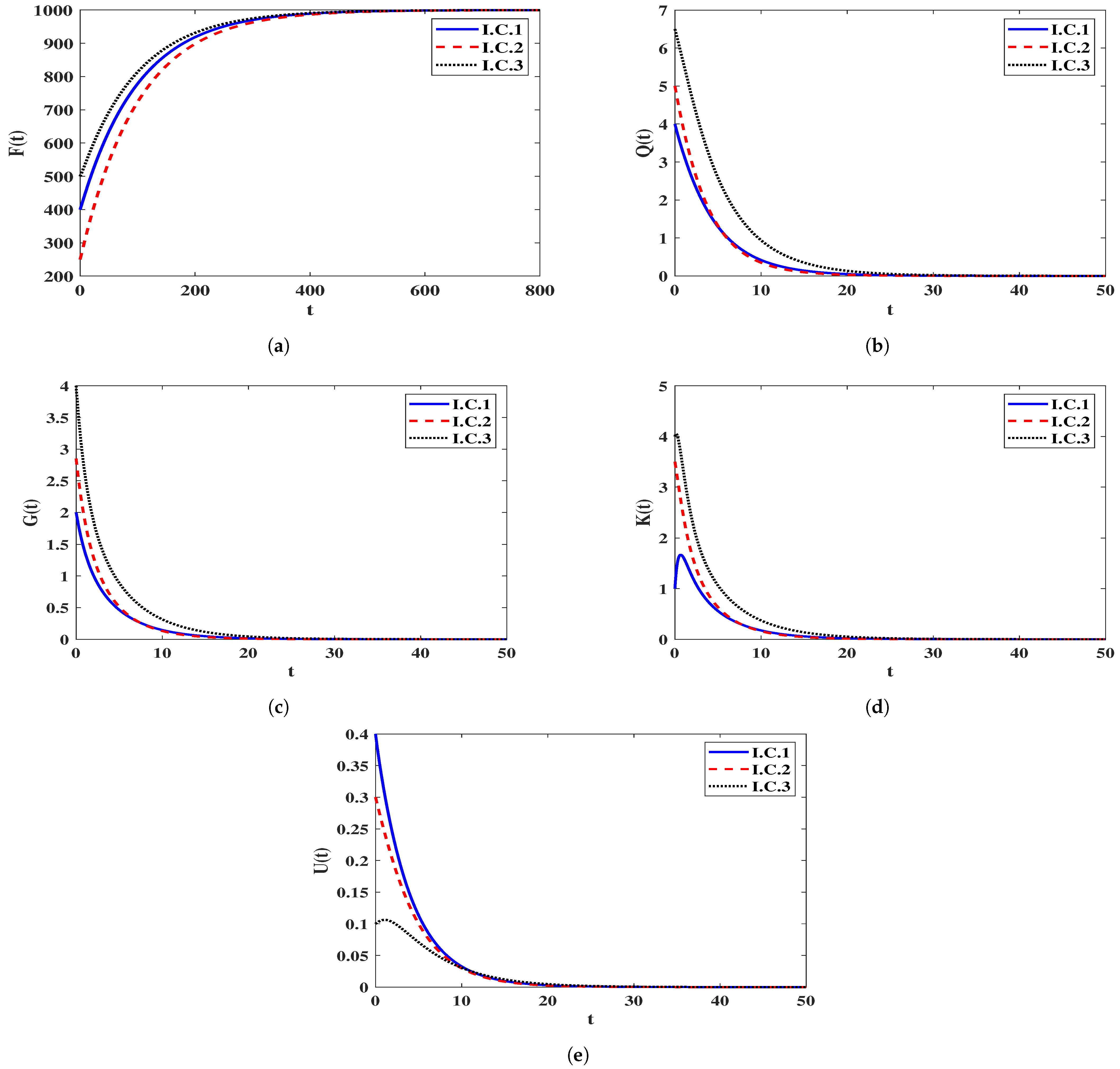
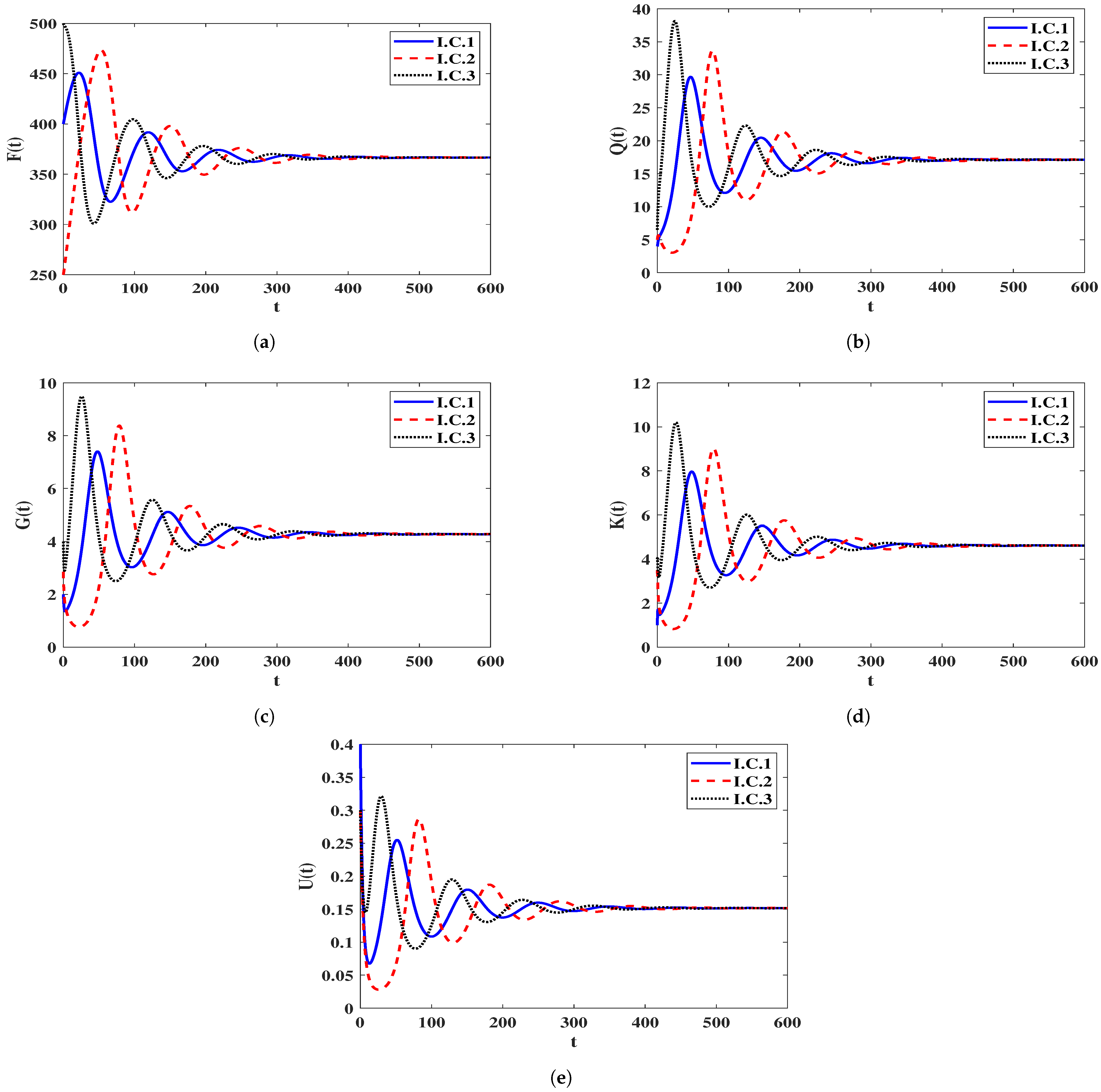
4.1.1. Stability of Equilibria

In this part, we perform numerical simulations of system (5) using the parameter values provided in Table 1. Many of these parameter values are adopted from prior research. The remaining parameters, denoted as φ i for i = 1 , 2 , 3 , are chosen specifically for the purpose of our numerical simulations. To assess the stability of the equilibria in system (5), we initiate the simulations with three distinct initial conditions, as outlined below:
I.C.1:  ( F ( 0 ) , Q ( 0 ) , G ( 0 ) , K ( 0 ) , U ( 0 ) ) = ( 400 , 4 , 2 , 1 , 0.4 ) ,
I.C.2:  ( F ( 0 ) , Q ( 0 ) , G ( 0 ) , K ( 0 ) , U ( 0 ) ) = ( 250 , 5 , 2.85 , 3.5 , 0.3 ) ,
I.C.3:  ( F ( 0 ) , Q ( 0 ) , G ( 0 ) , K ( 0 ) , U ( 0 ) ) = ( 500 , 6.5 , 4 , 4 , 0.1 ) .
As 0 is employed to regulate the stability of equilibria and is contingent on the infection rates φ i for i = 1 , 2 , 3 , we introduce variations to these parameters. We then proceed to examine two distinct scenarios:
Stability of  Ξ Q 0 . We let φ 1 = 0.0002 ,   φ 2 = 0.0001 ,   φ 3 = 0.0004 and ε = 0.001 . This gives 0 = 0.6869 < 1 . Figure 1 presents that the trajectories of the solution starting with I.C.1-I.C.3 end up at the equilibrium Ξ Q 0 = ( 1000 , 0 , 0 , 0 , 0 ) . In fact, this shows that Ξ Q 0 is G.A.S based to the result of Theorem 2. From a biological perspective, this scenario implies that the infection will be eradicated, and the human body will successfully eliminate the pathogen.
Stability of  Ξ Q 1 . We let φ 1 = 0.003 ,   φ 2 = 0.0001 ,   φ 3 = 0.0004 and ε = 0.001 . With such choice we get 0 = 2.7365 > 1 . Clearly, the equilibrium point Ξ Q 1 exists when 0 > 1 with Ξ Q 1 = ( 366.543 , 17.121 , 4.28 , 4.619 , 0.152 ) . Figure 2 demonstrates that the numerical outcomes come to an agreement with the result of Theorem 3 as the solutions of system (5) end up at Ξ Q 1 when 0 > 1 for all I.C.1–I.C.3. From a biological standpoint, this situation reveals that both HIV-1 particles and B-cells will continue to exist within the host organism.

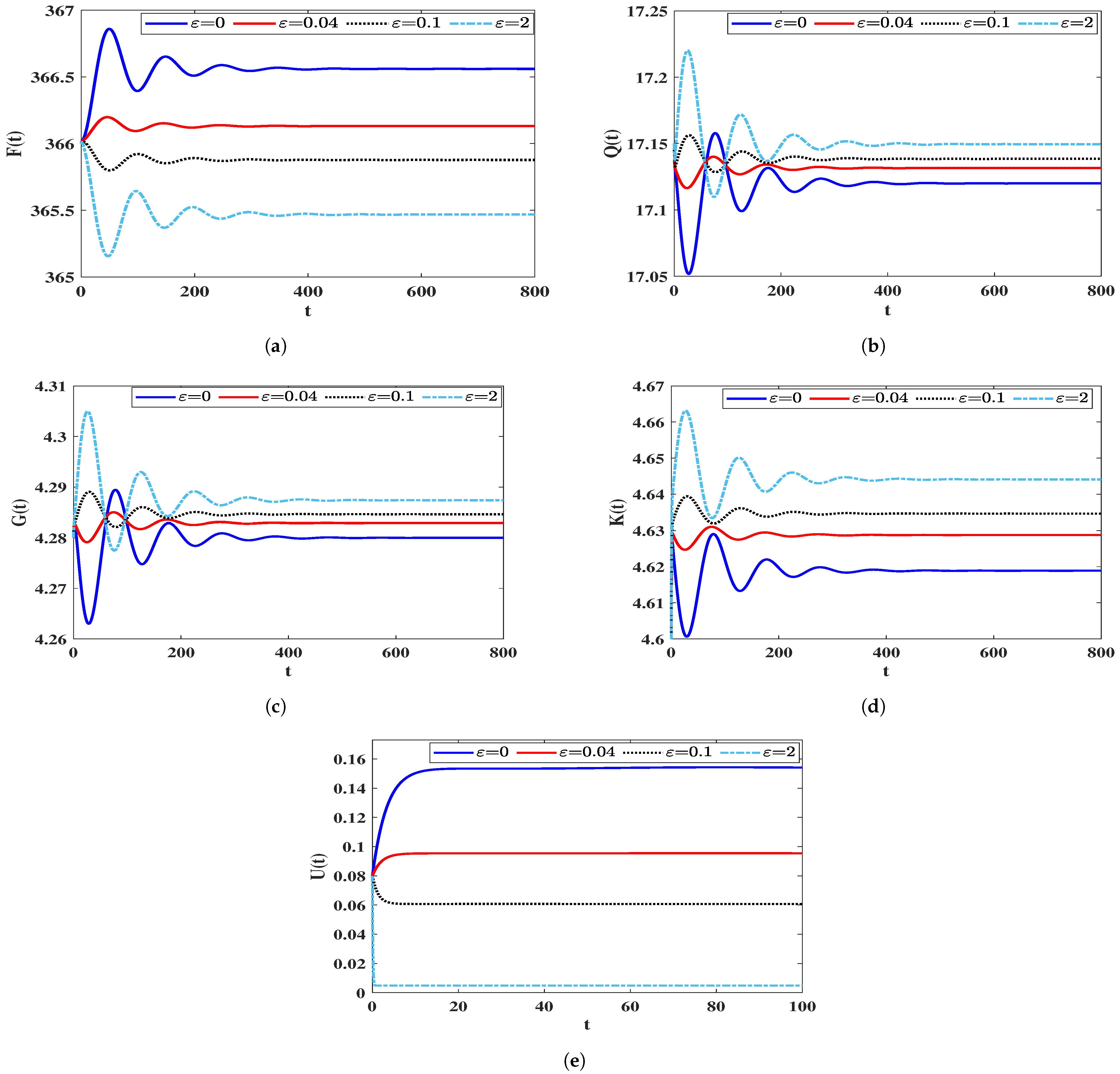
4.1.2. Effect of the Impaired Humoral Immunity

In this scenario, we introduce variations in the parameter ε while setting specific values for φ 1 = 0.003 , φ 2 = 0.0001 , and φ 3 = 0.0004 . To explore how the dynamics of system (5) are influenced by the impairment of the humoral immune response, we numerically solve the system, considering different values of ε as outlined in Table 2. In this case, we define the following initial condition:
I.C.4:  ( F ( 0 ) , Q ( 0 ) , G ( 0 ) , K ( 0 ) , U ( 0 ) ) = ( 366 , 17.15 , 4.28 , 4.6 , 0.08 ) .
We observe from Table 2 that an increase in ε results in a decrease in the number of B-cells. This reduction is linked to a higher count of (HIV-1)-latently and (HIV-1)-actively infected cells, as well as HIV-1 particles. As a consequence, the population of healthy CD4 + T cells decreases. An insightful observation from Figure 3 is that the impairment of the humoral immune response does not alter the stability criteria of the equilibria. This is evident as the parameter 0 remains unaffected by changes in ε .

4.2. Numerical Simulation for Model (23)

In this subsection, for numerical computations, we choose a specific form for the probability distribution functions T i ( λ ) , where i = 1 , 2 , 3 , as outlined below:
T i ( λ ) = δ * ( λ λ i ) , λ i 0 , ϱ i , i = 1 , 2 , 3 ,
where δ * ( . ) is the Dirac delta function. As ϱ i , we obtain
0 T i ( λ ) d λ = 1 , i = 1 , 2 , 3 .
Moreover, we have
Λ i = 0 δ * ( λ λ i ) e α i λ d λ = e α i λ i , i = 1 , 2 , 3 .
Therefore, the distributed-time delay system (23) will be converted into a discrete-time delay system as follows:
d F ( t ) d t = ψ ρ F ( t ) φ 1 F ( t ) K ( t ) φ 2 F ( t ) Q ( t ) φ 3 F ( t ) G ( t ) , d Q ( t ) d t = e α 1 λ 1 F ( t λ 1 ) ( φ 1 K ( t λ 1 ) + φ 2 Q ( t λ 1 ) + φ 3 G ( t λ 1 ) ) ( ξ + ϑ ) Q ( t ) , d G ( t ) d t = ξ e α 2 λ 2 Q ( t λ 2 ) θ G ( t ) , d K ( t ) d t = μ e α 3 λ 3 G ( t λ 3 ) κ K ( t ) σ U ( t ) K ( t ) , d U ( t ) d t = ϕ K ( t ) γ U ( t ) ε U ( t ) K ( t ) .
For system (40), the basic reproductive number is:
˜ 0 ( 40 ) = F ˜ 0 e α 1 λ 1 ξ e α 2 λ 2 φ 1 μ e α 3 λ 3 + φ 3 κ + φ 2 κ θ ξ + ϑ κ θ .

The Effect of the Time-Delays on the Stability of Equilibria

To explore how the solutions of the system are affected by the time-delay parameters (40), we keep the parameters constant φ 1 = 0.003 ,   φ 2 = 0.0001 ,   φ 3 = 0.0004 ,   ε = 0.001 ,   α 1 = 0.1 ,   α 2 = 0.2 and α 3 = 0.3 . On the contrary, the remaining parameters will be selected from Table 1. Furthermore, we will vary the delay parameters λ i , where i = 1 , 2 , 3 . The dependence of ˜ 0 ( 40 ) which is presented in Equation (41) on the values of λ i causes a remarkably changing in the stability of equilibria as long as parameters λ i are changed. Let’s consider the following scenarios for the delay values:
DV1  λ 1 = 0.07 , λ 2 = 0.06 , λ 3 = 0.05 .
DV2  λ 1 = 0.8 , λ 2 = 0.7 , λ 3 = 0.9 .
DV3  λ 1 = 1.3 , λ 2 = 1.4 , λ 3 = 1.5 .
DV4  λ 1 = 1.8 , λ 2 = 1.9 , λ 3 = 2 .
DV5  λ 1 = 4 , λ 2 = 3 , λ 3 = 5 .
We solve system (40) under the below initial
I.C.5:  ( F ( r ) , Q ( r ) , G ( r ) , K ( r ) , U ( r ) ) = ( 400 , 4 , 2 , 1 , 0.3 ) , r [ λ , 0 ] , λ = max { λ 1 , λ 2 , λ 3 } .
In Table 3, we present the values of ˜ 0 ( 40 ) for different values of λ i , i = 1 , 2 , 3 . We notice that an increase in the parameters λ i leads to a remarkable decrease in the values of ˜ 0 ( 40 ) . Figure 4 illustrates the numerical solutions of the system. A significant effect of the inclusion of time-delays is concluded, that is an increase in the number of healthy CD4 + T cells and a decrease in the numbers of (HIV-1)-latently and (HIV-1)-actively infected cells, HIV-1 particles, and B-cells occur.

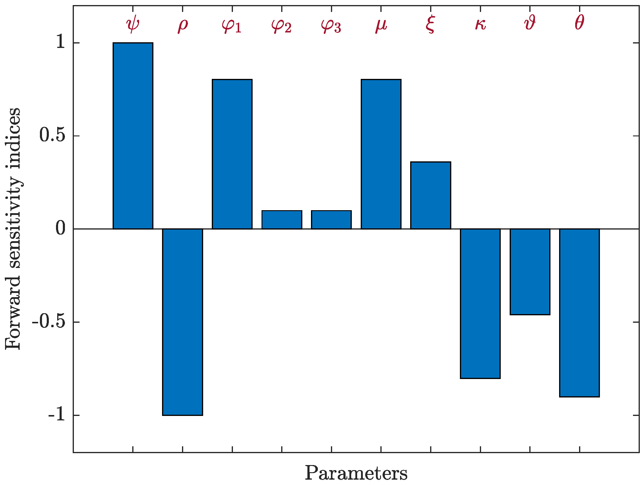
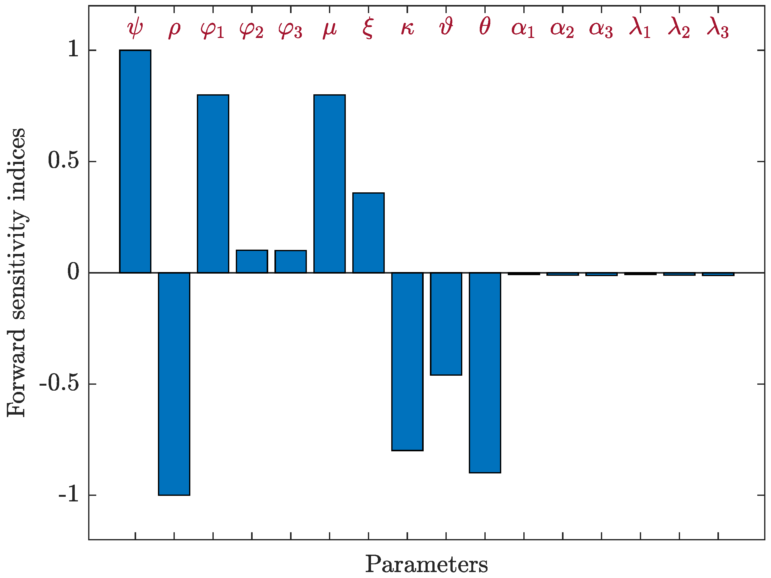
4.3. Sensitivity Analysis

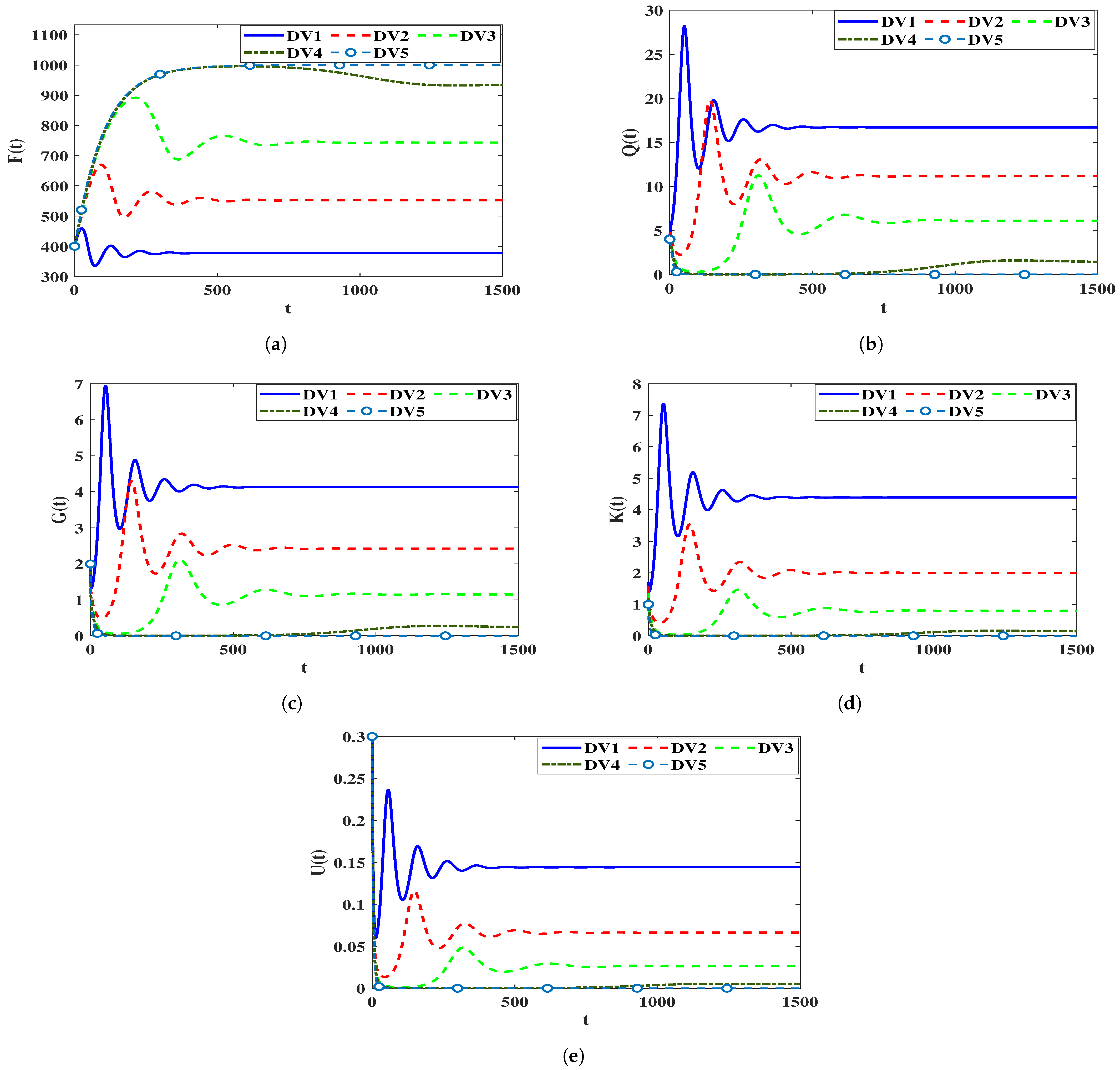
4.3.1. Sensitivity Analysis for Model (5)

The primary objective of a sensitivity analysis is to pinpoint the variable with the highest risk contribution. To achieve this, we will employ partial derivatives to compute sensitivity indices when variables undergo variations based on parameters. The normalized forward sensitivity index for the basic reproductive number, 0 , can be expressed in terms of parameters as follows:
Ξ S = S 0 0 S ,
where S is a given parameter. We used Equation (42) to determine the sensitivity indices for each parameter contained in the basic reproductive number, 0 , using the parameter values provided in Table 1, as well as the following parameters: φ 1 = 0.003 , φ 2 = 0.0001 and φ 3 = 0.0004 . Table 4 and Figure 5 present the sensitivity index values for 0 . It is evident that ψ , φ 1 , φ 2 , φ 3 , μ and ξ have positive indices values. In this instance, there is a correlation between the endemicity of the HIV-1 disease and an increase in the values of these parameters. The other indices are negative, which means that when the values of ρ , κ , ϑ and θ increase, the value of the basic reproductive number, 0 , decreases. Obviously, the most crucial parameters in terms of sensitivity are ψ , φ 1 and μ , while φ 2 and φ 3 are the least crucial. The parameter of B-cells responsiveness, ϕ , has no effect on 0 .

4.3.2. Sensitivity Analysis for Model (40)

We applied Equation (42) with respect to ˜ 0 ( 40 ) to compute the sensitivity indices for each parameter contained in the basic reproductive number, ˜ 0 ( 40 ) , using the parameter values provided in Table 1, as well as the following parameters: φ 1 = 0.003 , φ 2 = 0.0001 , φ 3 = 0.0004 , α 1 = 0.1 , α 2 = 0.2 , α 3 = 0.3 , λ 1 = 0.07 , λ 2 = 0.06 , and λ 3 = 0.05 . Table 5 and Figure 6 present the sensitivity index values for ˜ 0 ( 40 ) . Since, ψ , φ 1 , φ 2 , φ 3 , μ and ξ have positive indices, then, increasing these values will increase endemic of the HIV-1 disease. While increasing negative indices values, which are κ , ϑ , θ , α 1 , α 2 , α 3 , λ 1 , λ 2 , and λ 3 will decrease the value of ˜ 0 ( 40 ) . We can see that ψ , φ 1 and μ are the most important parameters, and φ 2 and φ 3 are the least important. The parameter of B-cells responsiveness, ϕ , has no effect on ˜ 0 ( 40 ) .

5. Discussion

To show the importance of including the latent CI spread in our proposed models, we consider model (5) under the effect of three types of antiviral drug therapies as:
d F ( t ) d t = ψ ρ F ( t ) ( 1 1 ) φ 1 F ( t ) K ( t ) ( 1 2 ) φ 2 F ( t ) Q ( t ) ( 1 3 ) φ 3 F ( t ) G ( t ) , d Q ( t ) d t = ( 1 1 ) φ 1 F ( t ) K ( t ) + ( 1 2 ) φ 2 F ( t ) Q ( t ) + ( 1 3 ) φ 3 F ( t ) G ( t ) ( ξ + ϑ ) Q ( t ) , d G ( t ) d t = ξ Q ( t ) θ G ( t ) , d K ( t ) d t = μ G ( t ) κ K ( t ) σ U ( t ) K ( t ) , d U ( t ) d t = ϕ K ( t ) γ U ( t ) ε U ( t ) K ( t ) ,
where 1 [ 0 , 1 ] is the efficacy of antiviral therapy in blocking VI. Moreover, 2 [ 0 , 1 ] and 3 [ 0 , 1 ] are the efficacies of therapy in blocking latent CI and active CI, respectively [50].
The basic reproductive number of system (43) is:
0 = ( 1 1 ) F 0 μ ξ φ 1 κ θ ξ + ϑ + ( 1 2 ) F 0 φ 2 ξ + ϑ + ( 1 3 ) F 0 ξ φ 3 θ ξ + ϑ .
We assume that = 1 = 2 = 3 , then we get
0 = ( 1 ) F 0 μ ξ φ 1 κ θ ξ + ϑ + F 0 φ 2 ξ + ϑ + F 0 ξ φ 3 θ ξ + ϑ = ( 1 ) 0 .
Now, we calculate the drug efficacy that makes 0 < 1 and stabilizes Ξ Q 0 of system (43) as:
1 > ˜ min = max 0 , 1 1 0 .
When we ignore the latent CI spread in model (43) we obtain
d F ( t ) d t = ψ ρ F ( t ) ( 1 ) φ 1 F ( t ) K ( t ) ( 1 ) φ 3 F ( t ) G ( t ) , d Q ( t ) d t = ( 1 ) φ 1 F ( t ) K ( t ) + ( 1 ) φ 3 F ( t ) G ( t ) ( ξ + ϑ ) Q ( t ) , d G ( t ) d t = ξ Q ( t ) θ G ( t ) , d K ( t ) d t = μ G ( t ) κ K ( t ) σ U ( t ) K ( t ) , d U ( t ) d t = ϕ K ( t ) γ U ( t ) ε U ( t ) K ( t ) ,
and the basic reproductive number of model (45) is:
^ 0 = ( 1 ) F 0 μ ξ φ 1 κ θ ξ + ϑ + F 0 ξ φ 3 θ ξ + ϑ = ( 1 ) ^ 0 .
We determine the drug efficacy that makes ^ 0 < 1 and stabilizes Ξ Q 0 of system (45) as:
1 > ^ min = max 0 , 1 1 ^ 0 .
Clearly, ^ 0 < 0 , then comparing Equations (44) and (46) we get that ^ min ˜ min . Therefore, if we apply drugs with efficacy such that ^ min < ˜ min , this guarantees that ^ 0 < 1 and then Ξ Q 0 of system (45) is G.A.S, however, 0 > 1 and then Ξ Q 0 of system (43) is unstable. Consequently, the designed drug therapies using a model without considering the latent CI spread may be inaccurate or insufficient to eradicate the viruses from the body. Therefore, our proposed models are more relevant in describing the HIV-1 dynamics than the models presented in [29,30].
The primary limitation of our current study is that we did not utilize real data to estimate the model’s parameter values. Several factors contribute to this limitation:
1.
Limited Availability of Real Data: There is a scarcity of real data from HIV-1 infected individuals, which hinders the accurate estimation of model parameters.
2.
Precision Issues: Comparing our obtained results with the limited existing studies may lack precision due to the scarcity of data points.
3.
Data Collection Challenges: Collecting real data from HIV-1 infected patients can be a challenging and resource-intensive task.
4.
Experimental Scope: Conducting experiments to obtain real data falls outside the scope of this paper.
Therefore, it is crucial to acknowledge that the theoretical findings presented in this paper should be validated against empirical observations when sufficient real data becomes accessible.

6. Conclusions

In this study, we developed two models to get an insight into HIV-1 dynamics taking impaired humoral immunity under consideration. These models consist of five compartments; healthy CD4 + T cells, (HIV-1)-latently infected cells, (HIV-1)-actively infected cells, free HIV-1 particles, and B-cells. In pursuit of a more realistic representation, we considered a scenario where healthy CD4 + T cells become susceptible to infection upon encountering free HIV-1 particles, (HIV-1)-latently infected cells, and (HIV-1)-actively infected cells. In our second model, we introduced three distributed time-delays to better capture the dynamics. It is noteworthy that the solutions generated by these models exhibit nonnegative and bounded characteristics. Within this framework, we identified two critical equilibria: the infection-free equilibrium denoted as Ξ Q 0 (or Ξ Q ˜ 0 ) and the infected equilibrium represented as Ξ Q 1 (or Ξ Q ˜ 1 ). To quantify the impact and potential outcomes, we computed the basic reproductive numbers, denoted as 0 (or ˜ 0 ). These values play a pivotal role in dictating the existence and global stability of the aforementioned equilibria. Notably, 0 (or ˜ 0 ) comprises three distinct components: the contribution from viral infection (VI), the contribution arising from latent cellular infection (latent CI), and the contribution attributed to active cellular infection (active CI). To assess the overall system behavior, we employed Lyapunov functions and the LaSalle’s invariance principle (L.I.P) to investigate the global asymptotic stability of these equilibria. Our analysis yielded two important scenarios: first, if 0 < 1 (or ˜ 0 < 1 ), then the infection-free equilibrium Ξ Q 0 (or Ξ Q ˜ 0 ) is globally asymptotically stable (G.A.S), leading to eventual infection extinction. Conversely, if 0 > 1 (or ˜ 0 > 1 ), the equilibrium Ξ Q 0 (or Ξ Q ˜ 0 ) becomes unstable, and the infected equilibrium Ξ Q 1 (or Ξ Q ˜ 1 ) prevails as G.A.S, signifying the establishment of chronic infection. To reinforce our theoretical findings, we conducted numerical simulations that corroborated our analytical results. Furthermore, we delved into the impact of B-cell impairment, time-delay, and latent CI on the dynamics of HIV-1. Notably, weakened immunity emerged as a significant contributor to disease progression. Additionally, the presence of time-delay emerged as a key factor in reducing the basic reproductive number ˜ 0 and consequently suppressing HIV-1 replication. In light of this, strategies aimed at eliminating HIV-1 from the body should prioritize measures that reduce ˜ 0 below 1. We also observed an increase in delay parameters λ i , where i = 1 , 2 , 3 , when infected patients undergo drug therapies against HIV-1. In a crucial finding, we highlighted the consequences of neglecting latent CI spread within the HIV-1 dynamics model. This omission can lead to an underestimation of the basic reproductive number, potentially resulting in inaccurate or insufficient drug dosing for virus eradication. This underscores the vital importance of incorporating latent CI spread within our proposed models. In addition, we conducted a sensitivity analysis to elucidate how variations in the values of all model parameters can impact 0 (or ˜ 0 ) under specific data conditions. This comprehensive analysis provided valuable insights into the sensitivity of the system to parameter changes, further enhancing our understanding of HIV-1 dynamics.

Future Works

The following enhancements can be made to extend Model (23):
  • Including the diffusion of the cells and viruses as [8,9]:
    F ( t , h ) t ϕ F Δ F t , h = ψ ρ F t , h φ 1 F t , h K t , h φ 2 F t , h Q t , h φ 3 F t , h G t , h , Q t , h t ϕ Q Δ Q t , h = 0 ϱ 1 T 1 λ e α 1 λ F t λ , h φ 1 K t λ , h + φ 2 Q t λ , h + φ 3 G t λ , h d λ ( ξ + ϑ ) Q t , h , G t , h t ϕ G Δ G t , h = ξ 0 ϱ 2 T 2 λ e α 2 λ Q t λ , h d λ θ G t , h , K t , h t ϕ K Δ K t , h = μ 0 ϱ 3 T 3 λ e α 3 λ G t λ , h d λ κ K t , h σ U ( t , h ) K ( t , h ) , U t , h t ϕ U Δ U t , h = ϕ K ( t , h ) γ U ( t , h ) ε U ( t , h ) K ( t , h ) ,
    where h is the position, Δ = 2 h 2 and ϕ u is the diffusion coefficient of compartment u. One can also include different kinds of diffusion in our systems (see e.g., [51,52,53]).
  • Utilizing real-world data to estimate model parameters accurately, which can enhance the model’s predictive capabilities and align it better with empirical observations.
  • Broadening the scope of the model to incorporate the role of Cytotoxic T Lymphocytes (CTLs) alongside B-cells, allowing for a more comprehensive representation of the immune response.
  • Investigating the integration of age structure into the infected cell population within the model, which can provide insights into how age-related factors impact disease dynamics.
  • Exploring the effects of viral mutations on the dynamics of the model, considering how genetic changes in the virus may influence disease progression and response to interventions.
It should be noted that these proposed enhancements are being deferred for future consideration and further study.

Author Contributions

Conceptualization, N.H.A. and A.M.E.; Methodology, N.H.A.; Software, N.H.A., R.H.H. and A.M.E.; Validation, N.H.A. and A.M.E.; Formal analysis, N.H.A. and R.H.H.; Investigation, N.H.A.; Resources, N.H.A. and A.M.E.; Writing—original draft, N.H.A., R.H.H. and A.M.E.; Writing—review & editing, W.S.; Visualization, N.H.A. and A.M.E.; Supervision, N.H.A. and A.M.E. All authors have read and agreed to the published version of the manuscript.

Funding

This work was funded by the University of Jeddah, Jeddah, Saudi Arabia, under grant No. (UJ-22-DR-102).

Data Availability Statement

Not applicable.

Acknowledgments

This work was funded by the University of Jeddah, Jeddah, Saudi Arabia, under grant No. (UJ-22-DR-102). The authors, therefore, acknowledge with thanks the University of Jeddah for its technical and financial support.

Conflicts of Interest

The authors declare that they have no conflict of interest regarding the publication of this paper.

References

  1. Wodarz, D.; Levy, D.N. Human immunodeficiency virus evolution towards reduced replicative fitness in vivo and the development of AIDS. Proc. R. Soc. Biol. Sci. 2007, 274, 2481–2491. [Google Scholar] [CrossRef]
  2. Available online: https://www.who.int/data/gho/data/themes/hiv-aids (accessed on 1 July 2023).
  3. Wodarz, D.; May, R.M.; Nowak, M.A. The role of antigen-independent persistence of memory cytotoxic T lymphocytes. Int. Immunol. 2000, 12, 467–477. [Google Scholar] [CrossRef]
  4. Elaiw, A.M.; AlShamrani, N.H. Global stability of humoral immunity virus dynamics models with nonlinear infection rate and removal. Nonlinear Anal. Real World Appl. 2015, 26, 161–190. [Google Scholar] [CrossRef]
  5. Wang, S.; Zou, D. Global stability of in host viral models with humoral immunity and intracellular delays. Appl. Math. Model. 2012, 36, 1313–1322. [Google Scholar] [CrossRef]
  6. Xu, J.; Zhou, Y.; Li, Y.; Yang, Y. Global dynamics of a intracellular infection model with delays and humoral immunity. Math. Methods Appl. Sci. 2016, 39, 427–5435. [Google Scholar] [CrossRef]
  7. Miao, H.; Teng, Z.; Kang, C.; Muhammadhaji, A. Stability analysis of a virus infection model with humoral immunity response and two time delays. Math. Methods Appl. Sci. 2016, 39, 3434–3449. [Google Scholar] [CrossRef]
  8. Tang, S.; Teng, Z.; Miao, H. Global dynamics of a reaction–diffusion virus infection model with humoral immunity and nonlinear incidence. Comput. Math. Appl. 2019, 78, 786–806. [Google Scholar] [CrossRef]
  9. Zheng, T.; Luo, Y.; Teng, Z. Spatial dynamics of a viral infection model with immune response and nonlinear incidence. Z. Angew. Math. Phys. 2023, 74, 124. [Google Scholar] [CrossRef] [PubMed]
  10. Duan, X.; Yuan, S. Global dynamics of an age-structured virus model with saturation effects. Math. Methods Appl. Sci. 2017, 40, 1851–1864. [Google Scholar] [CrossRef]
  11. Kajiwara, T.; Sasaki, T.; Otani, Y. Global stability for an age-structured multistrain virus dynamics model with humoral immunity. J. Appl. Math. Comput. 2020, 62, 239–279. [Google Scholar] [CrossRef]
  12. Avila-Vales, E.; Pérez, Á.G. Global properties of an age-structured virus model with saturated antibody-immune response, multi-target cells, and general incidence rate. Boletín Soc. Matemática Mex. 2021, 27, 26. [Google Scholar] [CrossRef]
  13. Nowak, M.A.; May, R.M. Virus Dynamics; Oxford University Press: New York, NY, USA, 2000. [Google Scholar]
  14. Inoue, T.; Kajiwara, T.; Sasaki, T. Global stability of models of humoral immunity against multiple viral strains. J. Biol. Dyn. 2010, 4, 282–295. [Google Scholar] [CrossRef] [PubMed]
  15. Dhar, M.; Samaddar, S.; Bhattacharya, P. Modeling the effect of non-cytolytic immune response on viral infection dynamics in the presence of humoral immunity. Nonlinear Dyn. 2019, 98, 637–655. [Google Scholar] [CrossRef]
  16. Dhar, M.; Samaddar, S.; Bhattacharya, P. Modeling the cell-to-cell transmission dynamics of viral infection under the exposure of non-cytolytic cure. J. Appl. Math. Comput. 2021, 65, 885–911. [Google Scholar] [CrossRef]
  17. Jolly, C.; Sattentau, Q. Retroviral spread by induction of virological synapses. Traffic 2004, 5, 643–650. [Google Scholar] [CrossRef]
  18. Sato, H.; Orenstein, J.; Dimitrov, D.; Martin, M. Cell-to-cell spread of HIV-1 occurs within minutes and may not involve the participation of virus particles. Virology 1992, 186, 712–724. [Google Scholar] [CrossRef]
  19. Iwami, S.; Takeuchi, J.S.; Nakaoka, S.; Mammano, F.; Clavel, F.; Inaba, H.; Kobayashi, T.; Misawa, N.; Aihara, K.; Koyanagi, Y.; et al. Cell-to-cell infection by HIV contributes over half of virus infection. eLife 2015, 4, e08150. [Google Scholar] [CrossRef]
  20. Komarova, N.L.; Wodarz, D. Virus dynamics in the presence of synaptic transmission. Math. Biosci. 2013, 242, 161–171. [Google Scholar] [CrossRef]
  21. Sourisseau, M.; Sol-Foulon, N.; Porrot, F.; Blanchet, F.; Schwartz, O. Inefficient human immunodeficiency virus replication in mobile lymphocytes. J. Virol. 2007, 81, 1000–1012. [Google Scholar] [CrossRef]
  22. Sigal, A.; Kim, J.T.; Balazs, A.B.; Dekel, E.; Mayo, A.; Milo, R.; Baltimore, D. Cell-to-cell spread of HIV permits ongoing replication despite antiretroviral therapy. Nature 2011, 477, 95–98. [Google Scholar] [CrossRef]
  23. Martin, N.; Sattentau, Q. Cell-to-cell HIV-1 spread and its implications for immune evasion. Curr. Opin. HIV AIDS 2009, 4, 143–149. [Google Scholar] [CrossRef]
  24. Lin, J.; Xu, R.; Tian, X. Threshold dynamics of an HIV-1 virus model with both virus-to-cell and cell-to-cell transmissions, intracellular delay, and humoral immunity. Appl. Math. Comput. 2017, 315, 516–530. [Google Scholar] [CrossRef]
  25. Luo, Y.; Zhang, L.; Zheng, T.; Teng, Z. Analysis of a diffusive virus infection model with humoral immunity, cell-to-cell transmission and nonlinear incidence. Phys. Stat. Mech. Its Appl. 2019, 535, 122415. [Google Scholar] [CrossRef]
  26. Lydyard, P.; Whelan, A.; Fanger, M. BIOS Instant Notes in Immunology; Taylor & Francis e-Library: Abingdon, UK, 2005. [Google Scholar]
  27. Miao, H.; Abdurahman, X.; Teng, Z.; Zhang, L. Dynamical analysis of a delayed reaction-diffusion virus infection model with logistic growth and humoral immune impairment. Chaos Solitons Fractals 2018, 110, 280–291. [Google Scholar] [CrossRef]
  28. Elaiw, A.M.; Alshehaiween, S.F.; Hobiny, A.D. Global properties of delay-distributed HIV dynamics model including impairment of B-cell functions. Mathematics 2019, 7, 837. [Google Scholar] [CrossRef]
  29. Elaiw, A.M.; Alshehaiween, S.F. Global stability of delay-distributed viral infection model with two modes of viral transmission and B-cell impairment. Math. Methods Appl. Sci. 2020, 43, 6677–6701. [Google Scholar] [CrossRef]
  30. Elaiw, A.M.; Alshehaiween, S.F.; Hobiny, A.D. Impact of B-cell impairment on virus dynamics with time delay and two modes of transmission. Chaos Solitons Fractals 2020, 130, 109455. [Google Scholar] [CrossRef]
  31. Miao, H.; Liu, R.; Jiao, M. Global dynamics of a delayed latent virus model with both virus-to-cell and cell-to-cell transmissions and humoral immunity. J. Inequalities Appl. 2021, 2021, 156. [Google Scholar] [CrossRef]
  32. Elaiw, A.M.; AlShamrani, N.H. Stability of a general adaptive immunity virus dynamics model with multi-stages of infected cells and two routes of infection. Math. Methods Appl. Sci. 2020, 43, 1145–1175. [Google Scholar] [CrossRef]
  33. Elaiw, A.M.; AlShamrani, N.H. Global stability of a delayed adaptive immunity viral infection with two routes of infection and multi-stages of infected cells. Commun. Nonlinear Sci. Numer. Simul. 2020, 86, 105259. [Google Scholar] [CrossRef]
  34. Agosto, L.; Herring, M.; Mothes, W.; Henderson, A. HIV-1-infected CD4+ T cells facilitate latent infection of resting CD4+ T cells through cell-cell contact. Cell Rep. 2018, 24, 2088–2100. [Google Scholar] [CrossRef]
  35. Wang, W.; Wang, X.; Guo, K.; Ma, W. Global analysis of a diffusive viral model with cell-to-cell infection and incubation period. Math. Methods Appl. Sci. 2020, 43, 5963–5978. [Google Scholar] [CrossRef]
  36. Alshamrani, N.H. Stability of a general adaptive immunity HIV infection model with silent infected cell-to-cell spread. Chaos Solitons Fractals 2021, 150, 110422. [Google Scholar] [CrossRef]
  37. Elaiw, A.M.; AlShamrani, N.H. Stability of a delayed adaptive immunity hiv infection model with silent infected cells and cellular infection. J. Appl. Anal. Comput. 2021, 11, 964–1005. [Google Scholar] [CrossRef] [PubMed]
  38. Hattaf, K.; Dutta, H. Modeling the dynamics of viral infections in presence of latently infected cells. Chaos Solitons Fractals 2020, 136, 109916. [Google Scholar] [CrossRef]
  39. van den Driessche, P.; Watmough, J. Reproduction numbers and sub-threshold endemic equilibria for compartmental models of disease transmission. Math. Biosci. 2002, 180, 29–48. [Google Scholar] [CrossRef]
  40. Willems, J.L. Stability Theory of Dynamical Systems; Wiley: New York, NY, USA, 1970. [Google Scholar]
  41. Korobeinikov, A. Global properties of basic virus dynamics models. Bull. Math. Biol. 2004, 66, 879–883. [Google Scholar] [CrossRef] [PubMed]
  42. Hale, J.K.; Lunel, S.M.V. Introduction to Functional Differential Equations; Springer: New York, NY, USA, 1993. [Google Scholar]
  43. Kuang, Y. Delay Differential Equations with Applications in Population Dynamics; Academic Press: San Diego, CA, USA, 1993. [Google Scholar]
  44. Hetmaniok, E.; Pleszczyński, M. Comparison of the selected methods used for solving the ordinary differential equations and their systems. Mathematics 2022, 10, 306. [Google Scholar] [CrossRef]
  45. Hetmaniok, E.; Pleszczyński, M.; Khan, Y. Solving the integral differential equations with delayed argument by using the DTM method. Sensors 2022, 22, 4124. [Google Scholar] [CrossRef]
  46. Sahani, S.K.; YASHI. Effects of eclipse phase and delay on the dynamics of HIV infection. J. Biol. Syst. 2018, 26, 421–454. [Google Scholar] [CrossRef]
  47. Wang, S.; Song, X.; Ge, Z. Dynamics analysis of a delayed viral infection model with immune impairment. Appl. Math. Model. 2011, 35, 4877–4885. [Google Scholar] [CrossRef]
  48. Allali, K.; Danane, J. Global analysis for an HIV infection model with CTL immune response and infected cells in eclipse phase. Appl. Sci. 2017, 7, 861. [Google Scholar] [CrossRef]
  49. Sun, C.; Li, L.; Jia, J. Hopf bifurcation of an HIV-1 virus model with two delays and logistic growth. Math. Model. Nat. Phenom. 2020, 15, 16. [Google Scholar] [CrossRef]
  50. Wang, X.; Rong, L. HIV low viral load persistence under treatment: Insights from a model of cell-to-cell viral transmission. Appl. Math. Lett. 2019, 94, 44–51. [Google Scholar] [CrossRef]
  51. Bellomo, N.; Painter, K.J.; Tao, Y.; Winkler, M. Occurrence vs. Absence of taxis-driven instabilities in a May-Nowak model for virus infection. SIAM J. Appl. Math. 2019, 79, 1990–2010. [Google Scholar] [CrossRef]
  52. Ren, X.; Tian, Y.; Liu, L.; Liu, X. A reaction-diffusion within-host HIV model with cell-to-cell transmission. J. Math. Biol. 2018, 76, 831–1872. [Google Scholar] [CrossRef]
  53. Bellomo, N.; Outada, N.; Soler, J.; Tao, Y.; Winkler, M. Chemotaxis and cross-diffusion models in complex environments: Models and analytic problems toward a multiscale vision. Math. Model. Methods Appl. Sci. 2022, 32, 713–792. [Google Scholar] [CrossRef]
Figure 1. Solutions F t , Q t , G t , K t , U t of system (5) whenever 0 < 1 . (a) Healthy CD 4 + T cells; (b) (HIV-1)-latently infected cells; (c) (HIV-1)-actively infected cells; (d) HIV-1 particles; (e) B-cells.
Computation 11 00207 g001
Figure 2. Solutions F t , Q t , G t , K t , U t of system (5) whenever 0 > 1 . (a) Healthy CD 4 + T cells; (b) (HIV-1)-latently infected cells; (c) (HIV-1)-actively infected cells; (d) HIV-1 particles; (e) B-cells.
Computation 11 00207 g002
Figure 3. Solutions of system (5) for various ε values. (a) Healthy CD 4 + T cells; (b) (HIV-1)-latently infected cells; (c) (HIV-1)-actively infected cells; (d) HIV-1 particles; (e) B-ells.
Computation 11 00207 g003
Figure 4. The influence of the time-delay parameters λ i on the solutions of the system (40). (a) Healthy CD 4 + T cells; (b) (HIV-1)-latently infected cells; (c) (HIV-1)-actively infected cells; (d) HIV-1 particles; (e) B-cells.
Computation 11 00207 g004
Figure 5. Forward sensitivity analysis of the parameters on 0 in system (5).
Computation 11 00207 g005
Figure 6. Forward sensitivity analysis of the parameters on ˜ 0 ( 40 ) of system (40).
Computation 11 00207 g006
Table 1. Model parameters.
ParameterValueReferenceParameterValueReference
ψ 10[46] θ 0.8 [47]
ρ 0.01 [46] μ 2.6 [48]
φ 1 varied- κ 2.4 [48]
φ 2 varied- σ 0.06 [49]
φ 3 varied- ϕ 0.01 [46]
ξ 0.2 [46] γ 0.3 [46]
ϑ 0.17 [46] ε varied-
Table 2. Effect of the impaired humoral immunity parameter.
ε Equilibria
ε = 0 Ξ Q 1 = ( 366.56 , 17.12 , 4.28 , 4.619 , 0.154 )
ε = 0.04 Ξ Q 1 = 366.131 , 17.132 , 4.283 , 4.629 , 0.095
ε = 0.1 Ξ Q 1 = 365.877 , 17.139 , 4.285 , 4.635 , 0.061
ε = 2 Ξ Q 1 = 365.468 , 17.15 , 4.287 , 4.644 , 0.005
Table 3. The disparity of ˜ 0 ( 40 ) based on λ i .
Delay Parameters ( λ 1 , λ 2 , λ 3 ) Equilibria ˜ 0 ( 40 )
( 0.07 , 0.06 , 0.05 ) Ξ Q ˜ 1 ( 40 ) = ( 377.574 , 16.705 , 4.126 , 4.388 , 0.144 ) ˜ 0 ( 40 ) = 2.656
( 0.8 , 0.7 , 0.9 ) Ξ Q ˜ 1 ( 40 ) = ( 552.652 , 11.161 , 2.426 , 2.003 , 0.066 ) ˜ 0 ( 40 ) = 1.812
( 1.3 , 1.4 , 1.5 ) Ξ Q ˜ 1 ( 40 ) = ( 743.32 , 6.092 , 1.151 , 0.795 , 0.026 ) ˜ 0 ( 40 ) = 1.346
( 1.8 , 1.9 , 2 ) Ξ Q ˜ 1 ( 40 ) = ( 935.941 , 1.446 , 0.247 , 0.147 , 0.005 ) ˜ 0 ( 40 ) = 1.069
( 4 , 3 , 5 ) Ξ Q ˜ 0 ( 40 ) = ( 1000 , 0 , 0 , 0 , 0 ) ˜ 0 ( 40 ) = 0.461
Table 4. Sensitivity index of 0 of model (5).
Parameter SValue of Ξ S Parameter SValue of Ξ S
ψ 1 μ 0.802
ρ 1 ξ 0.361
φ 1 0.802 κ 0.802
φ 2 0.099 ϑ 0.459
φ 3 0.099 θ 0.901
Table 5. Sensitivity index of ˜ 0 ( 40 ) of model (40).
Parameter SValue of Ξ S Parameter SValue of Ξ S
ψ 1 ϑ 0.459
ρ 1 θ 0.899
φ 1 0.799 α 1 0.007
φ 2 0.101 α 2 0.011
φ 3 0.1 α 3 0.012
μ 0.8 λ 1 0.007
ξ 0.358 λ 2 0.011
κ 0.799 λ 3 0.012
Disclaimer/Publisher’s Note: The statements, opinions and data contained in all publications are solely those of the individual author(s) and contributor(s) and not of MDPI and/or the editor(s). MDPI and/or the editor(s) disclaim responsibility for any injury to people or property resulting from any ideas, methods, instructions or products referred to in the content.

