Mathematical Investigation of the Infection Dynamics of COVID-19 Using the Fractional Differential Quadrature Method

Abstract

In recent times, the global community has been faced with the unprecedented challenge of the coronavirus disease (COVID-19) pandemic, which has had a profound and enduring impact on both global health and the global economy. The utilization of mathematical modeling has become an essential instrument in the characterization and understanding of the dynamics associated with infectious illnesses. In this study, the utilization of the differential quadrature method (DQM) was employed in order to anticipate the characterization of the dynamics of COVID-19 through a fractional mathematical model. Uniform and non-uniform polynomial differential quadrature methods (PDQMs) and a discrete singular convolution method (DSCDQM) were employed in the examination of the dynamics of COVID-19 in vulnerable, exposed, deceased, asymptomatic, and recovered persons. An analysis was conducted to compare the methodologies used in this study, as well as the modified Euler method, in order to highlight the superior efficiency of the DQM approach in terms of code-execution times. The results demonstrated that the fractional order significantly influenced the outcomes. As the fractional order tended towards unity, the anticipated numbers of vulnerable, exposed, deceased, asymptomatic, and recovered individuals increased. During the initial week of the inquiry, there was a substantial rise in the number of individuals who contracted COVID-19, which was primarily attributed to the disease’s high transmission rate. As a result, there was an increase in the number of individuals who recovered, in tandem with the rise in the number of infected individuals. These results highlight the importance of the fractional order in influencing the dynamics of COVID-19. The utilization of the DQM approach, characterized by its proficient code-execution durations, provided significant insights into the dynamics of COVID-19 among diverse population cohorts and enhanced our comprehension of the evolution of the pandemic. The proposed method was efficient in dealing with ordinary differential equations (ODEs), partial differential equations (PDEs), and fractional differential equations (FDEs), in either linear or nonlinear forms. In addition, the stability of the DQM and its validity were verified during the present study. Moreover, the error analysis showed that DQM has better error percentages in many applications than other relevant techniques.

1. Introduction

The vast genome of the viruses known as coronaviruses consists of non-segmented, single-stranded, positive-sense ribonucleic acid (RNA) and is contained inside an envelope. The viruses share features with other members of the Nidovirales order, including the ability to express genes through a three-nested set of numerous sub-genomic messenger RNAs (mRNAs), the presence of a ribosomal frameshifting mechanism, the presence of distinctive enzymatic activity, the development of a virion envelope, and the presence of a multi-span membrane protein inside the virion. The 28 species of coronaviruses are divided into three groups, with groups 1 and 2 being found in mammals and group 3 being found in birds. The first human coronaviruses (hCoVs), hCoV-229E and hCoV-OC43, were discovered in the lungs of humans in the 1960s. In the early 2000s, however, a coronavirus associated with severe acute respiratory syndrome (SARS-CoV) triggered an epidemic of SARS, resulting in 776 fatalities and a case fatality rate (CFR) of 9.6%. This marked the transition of coronaviruses from being relatively harmless to being extremely pathogenic to humans.

Since the inception of the continuing COVID-19 pandemic in 2013, about 7,000,000 people have died. This pandemic was further fueled by the outbreak of Middle East respiratory syndrome (MERS) in 2012. Coronaviruses were divided into four subgroups, based on phylogenetic analyses: alpha, beta, gamma, and delta. Six human coronaviruses (hCoVs) related to alphacoronaviruses (hCoV-229E and hCoV-NL63) or betacoronaviruses (hCoV-OC43, hCoV-HKU1, MERS-CoV, and SARS-CoV) were reported prior to the emergence of the novel coronavirus in 2019. Because of its structural and pathological similarities to SARS-CoV, the new hCoV that causes COVID-19 is categorized as a betacoronavirus, named SARS-CoV-2. According to reports, zoonotic hCoVs that caused outbreaks circulated in animals before spreading to people. In Wuhan, China, at the end of December 2019, SARS-CoV-2 first appeared. The presence of SARS-CoV in bats, palm civets, and raccoon dogs is particularly noteworthy. Additionally, bats can spread MERS-CoV, although camels are its primary host.

According to human epidemiological data, a sizable portion of first- and second-generation human cases of COVID-19 were linked to the Huanan Seafood Wholesale Market in Wuhan, China. Following whole-genome sequencing, which revealed 96.2% similarity, it was determined that SARS-CoV-2 was linked to bat coronavirus RaTG13 (Bat-CoV RaTG13) [1].

On 11 March 2020, the World Health Organization (WHO) declared that the outbreak of COVID-19 was a pandemic. By the middle of April 2021, over 137 million confirmed cases and over 2.95 million fatalities globally prompted a global public health emergency that was caused by this deadly viral illness. This epidemic has affected almost 229 nations, regions, and territories. Being a respiratory ailment that is extremely infectious and has the potential to be quite severe, COVID-19 has presented considerable problems to public health systems all over the world [2].

Mathematical modeling is an essential part of understanding the dynamics of virus transmission, predicting the path the virus will take in the future, and developing control methods that are both efficient and effective. In 2020, Chen et al. [3] developed a mathematical model to simulate the potential transmission of COVID-19 from the infection source to human beings. The model was based on the assumption that COVID-19 is transmitted from bats to wild animals as hosts, with transmission to humans after they hunted through seafood markets. The model was a system of ordinary differential equations (ODEs).

Derivatives and integrals of fractional order are the focus of fractional calculus (FC). Derivatives and integrals of fractional order are as ancient as calculus itself, but they have had a renaissance in the last thirty years due to their widespread use in fields as diverse as physics, biology, and sociology. The solutions of differential equations of fractional order more accurately represent practical circumstances than their integer-order counterparts. Because the biological models incorporating derivatives are more realistic and complete than the conventional order models, Caputo fractional order derivative (CFOD)-based models have received much interest in recent years. Several types of difficulties have been investigated in this context, including qualitative theory, analytical solutions, and numerical calculations. Many methods have been developed to deal with these issues. Hybrid methods, including the integration transform and other approaches, such as perturbations or decompositions, have become popular in dealing with linear and nonlinear problems of fractional order [4,5,6,7]. Yasmin et al. [8,9] constructed families of solutions of fractional models, using an extended direct algebraic method. In addition, a long-waves model by fractional derivatives were investigated by Naeem et al. [10].

For more generalization, the Caputo fractional order derivative model has been developed to fully describe COVID-19. Nazir et al. [11] studied the fractional model using a modified Euler method and Mpinganzima et al. [12,13] numerically investigated the prediction model in Rwanda for the impact of control measures. Abioye et al. [14] analyzed the mathematical model for malaria and COVID-19 using a two-step Lagrange interpolation polynomial approximate method. Their findings demonstrated that decreasing the likelihood of developing malaria and COVID-19 through preventative measures reduced the risk of contracting COVID-19 following malaria infection and decreased the risk of contracting malaria following COVID-19 infection, to the point of elimination. The spatiotemporal spread of COVID-19 in the presence of vaccine distribution was examined mathematically by Alaje et al. [15] via a homotopy perturbation method. A spatiotemporal study of population states underscored the importance of comprehensive vaccination coverage in eradicating COVID-19 globally. Avusuglo et al. [16] examined a mathematical model of COVID-19 and influenza in Canada. The results indicated that the influenza vaccination rate and the transmission rates for both COVID-19 and influenza had a lower and approximately similar effect on absenteeism. In contrast, the rate of COVID-19 immunization and the capacity for polymerase-chain-reaction (PCR) testing were critical determinants for lowering absenteeism. Moreover, the authors utilized the model to estimate and quantify the (indirect) advantage of influenza vaccination against the spread of COVID-19. Singh et al. [17] studied the transmission dynamics of COVID-19 and tuberculosis via a Runge–Kutta fourth-order method. The results showed that both infections can be mitigated by controlling the transmission rate.

The aim of this study is to employ a more reliable technique—the differential quadrature method (DQM)—and modify it to suit the fractional models which are known as fractional DQMs. Uniform and non-uniform polynomial differential quadrature methods (PDQMs) and a discrete singular convolution method (DSCDQM) are employed to reduce the execution time and errors more than can be achieved by relevant numerical techniques. These techniques are employed to describe and investigate the dynamical behavior of COVID-19 to estimate the numbers of susceptible, exposed, deceased, asymptomatic, and recovered people. Moreover, the effect of fractional order is considered throughout the investigation process.

The current manuscript is organized as follows: Section 2 is devoted to describing the mathematical formulation of the model. In Section 3, the differential quadrature method is introduced for fractional differential equations. The numerical results are described in Section 4 and the conclusions are stated in Section 5.

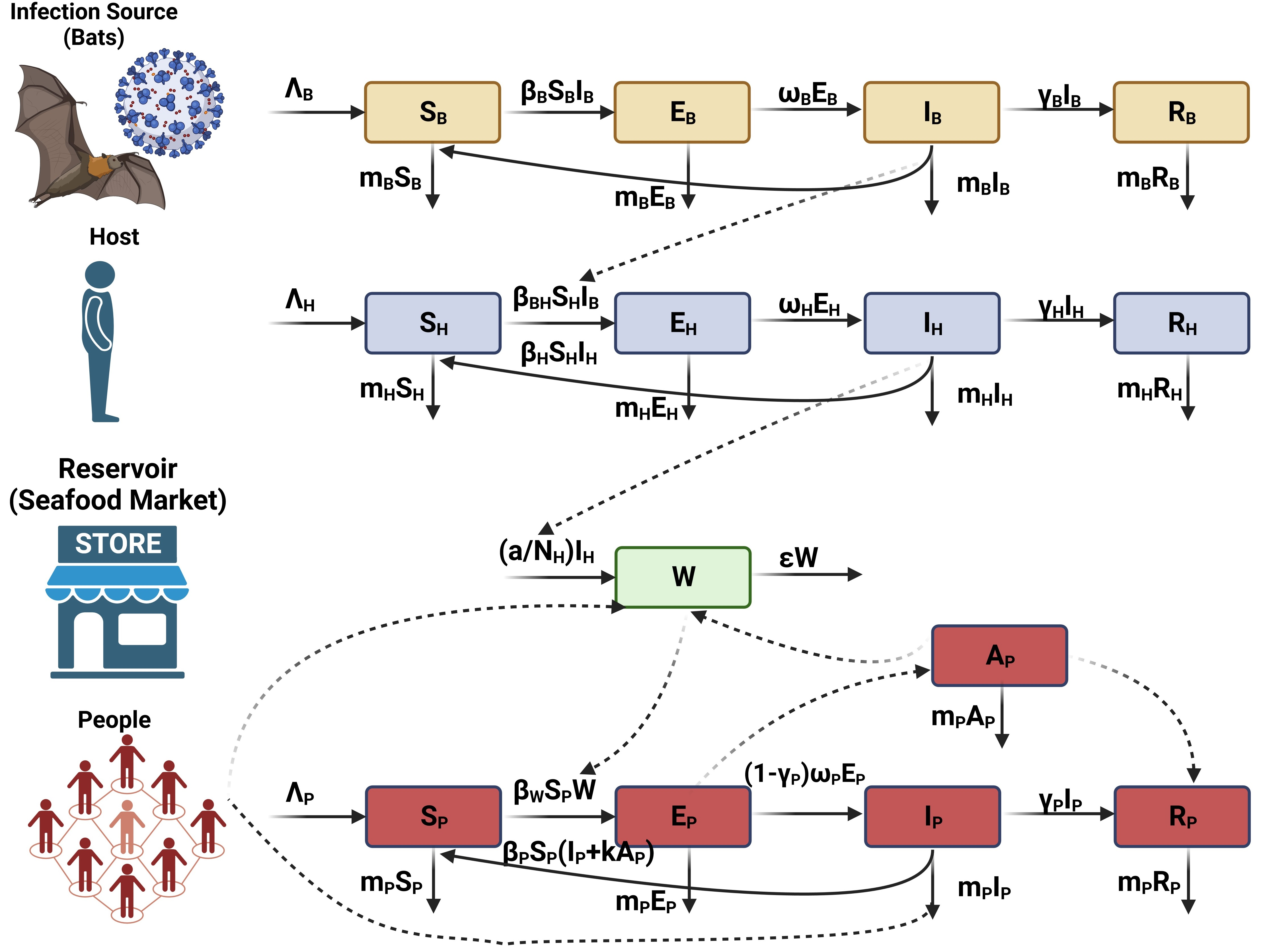
2. Mathematical Model of COVID-19

The mathematical model describing the dynamics of infection for COVID-19 is described by the following fractional order system, with order $0<\eta <1$ [11]:

$${ }^c{D}^{\eta }{S}_p\left(t\right)={\mathsf{\Lambda }}_p-m_p{S}_p-{\beta }_p{S}_p\left(I_p+k{A}_p\right)-{\beta }_W{S}_{P}W,$$

(1)

$${ }^c{D}^{\eta }{E}_p\left(t\right)={\beta }_p{S}_p\left(I_p+k{A}_p\right)+{\beta }_W{S}_{p}W-\left(1-{\delta }_p\right){\omega }_p{E}_p-{\delta }_p{\acute{\omega }}_p{E}_p-m_p{E}_p,$$

(2)

$${ }^c{D}^{\eta }{I}_p\left(t\right)=\left(1-{\delta }_p\right){\omega }_p{E}_p-\left({\gamma }_p+m_p\right)I_p,$$

(3)

$${ }^c{D}^{\eta }{A}_p\left(t\right)={\delta }_p{\acute{\omega }}_p{E}_p-\left({\acute{\gamma }}_p+m_p\right)A_p,$$

(4)

$${ }^c{D}^{\eta }{R}_p\left(t\right)={\gamma }_p{I}_p+{\acute{\gamma }}_p{A}_p-m_p{R}_p,$$

(5)

$${ }^c{D}^{\eta }W\left(t\right)={\mu }_p{I}_p+{\acute{\mu }}_p{A}_p-\epsilon W,$$

(6)

where ${ }^c{D}^{\eta }$ refers to Caputo’s fractional derivative of order $\eta$. The population is divided into five epidemiological compartments: susceptible people $S_p$, exposed people $E_p$, symptomatic infected people $I_p$, asymptomatic infected people $A_p$ and removed people $R_p$ (including recovered and deceased people). $W$ represents the reservoir of the virus. Moreover, ${\mathsf{\Lambda }}_p$ is the total population and birth date, $m_p$ is the rate of death, ${\beta }_p$ is the transmission rate from $I_p$ to $S_p$, $k$ is the multiple of the transmissibility of $A_p$ to that of $I_p$, ${\beta }_w$ is the transmission rate from $W$ to $S_p$, ${\delta }_p$ is the proportion of the asymptomatic infection rate of people, ${\omega }_p$ is the incubation period, ${\acute{\omega }}_p$ is the latent period, ${\gamma }_p$ is the infectious period of symptomatic infection, ${\acute{\gamma }}_p$ is the infectious period of asymptomatic infection of people, ${\mu }_p$ is the shedding coefficients from $I_p$ to $W$, ${\acute{\mu }}_p$ represents the shedding coefficients from $A_p$ to $W$, and $\epsilon$ is the lifetime of the virus in W.

The initial conditions are as follows:

$$S_p\left(0\right)=S_{P_0},E_p\left(0\right)=E_{P0},I_p\left(0\right)=I_{P_0},A_p\left(0\right)=A_{p_0},R_p\left(0\right)=R_{p_0},W\left(0\right)=W_0.$$

(7)

3. Preliminaries and Method of Solution

Here, the system of fractional order differential Equations (1)–(6) is solved by the fractional differential quadrature method (FDQM) with two distinct shape functions. First, Caputo’s fractional derivative is introduced; then, the FDQM is described and applied.

3.1. Caputo’s Fractional Derivative

In ordinary calculus, the focus is on higher order derivatives $D^{n}f=\frac{d^{n}f}{d{x}^n}$, where is the convention is that $D^{0}f=f$. These derivatives are typically considered only when $n\in N$, which means $n$ belongs to the set of natural numbers. However, there is a natural extension of calculus that aims to define derivatives and integrals with arbitrary real orders α > 0, encompassing the ordinary definitions as special cases. This field is known as fractional calculus, and its origins trace back to 1695 when L’Hospital posed the question to Leibniz regarding the meaning of $\frac{d^{\raisebox{1ex}{$1$}\!\left/ \!\raisebox{-1ex}{$2$}\right.}}{d{x}^{\raisebox{1ex}{$1$}\!\left/ \!\raisebox{-1ex}{$2$}\right.}}$. For over two centuries, fractional calculus remained primarily within the realm of pure mathematics, with notable mathematicians like Euler, Fourier, Abel, Liouville, Riemann, and Hadamard studying these fractional operators, introducing new definitions, and investigating their fundamental properties.

However, in recent decades, the practical applications of fractional calculus have become evident in various natural phenomena.

Definition 1.

The Riemann–Liouville derivative of fractional order $\eta$ [18], for a function $\upsilon \left(t\right),$ is defined as:

$${}^{RL}{D}_a^{\eta }\upsilon \left(t\right)=\frac{1}{\Gamma \left(k-\eta \right)}\frac{d^k}{d{t}^k}\underset{a}{\overset{t}{{\displaystyle \int }}}{\left(t-x\right)}^{k-\eta -1}\upsilon \left(x\right)dx,\hspace{1em}k-1\le \eta <k\in R^{+},$$

(8)

In his 1967 paper [19], Caputo introduced a reformulation of the Riemann–Liouville fractional derivative. He achieved this by interchanging the order of the ordinary derivative and the fractional integral operator. This modification resulted in a Laplace transform of the derivative that now incorporates integer-order initial conditions, in contrast to the fractional-order conditions associated with the Riemann–Liouville fractional derivative. Inspired by this concept, Caputo’s fractional-derivative definition based on the Riemann–Liouville (RL) derivative is defined as follows:

Definition 2.

The Caputo derivative [18] of fractional order $\eta$ of a function $\upsilon \left(t\right)$ is defined as:

$${ }^c{D}^{\eta }\upsilon \left(t\right)=\{\begin{array}{c}\frac{1}{\Gamma \left(k-\eta \right)}\underset{a}{\overset{t}{{\displaystyle \int }}}{\left(t-x\right)}^{k-\eta -1} {\upsilon }^{\left(k\right)}\left(x\right)dx,\hspace{1em}k-1<\eta <k \in R^{+},\\ \frac{d^k\upsilon }{d{t}^k},\hspace{1em}k=\eta .\end{array}$$

(9)

where $a$ is the integration lower limit. For $\lambda =\kappa$, the classical definition of the integer-order derivative is obtained.

3.2. Polynomial Based Differential Quadrature Method

The FDQM is a powerful numerical method that discretizes the fractional derivatives present in the equations. This method involves approximating the derivatives using discrete points and shape functions. The selection of appropriate shape functions is crucial in ensuring the accuracy and convergence of the numerical solution. By employing the FDQM, the fractional-order differential equations system is transformed into a system of algebraic equations. Employing FDQM allows the numerical solution to be obtained using standard techniques, such as matrix operations and iterative methods. The FDQM is particularly effective in handling fractional-order equations, as it can accurately capture the non-local effects and memory-dependent behavior inherent in such systems.

Bellman et al. [20] extended the Gauss quadrature technique to find the derivatives of numerous orders of any differentiable function. They approximated the derivatives of the function by a weighted sum of the function values at a group of nodes. Suppose a function $\upsilon \left(t\right)$ is sufficiently smooth on the interval [$t_1$, $t_N$]:

Then, the different derivatives of this function can be determined as follows [20]:

$$\frac{{\partial }^n\upsilon }{\partial t^n}{|}_{t=t_i}={\sum }_{j=1}^N{\Re }_{ij}^{\left(n\right)}\upsilon \left(t_j\right),\left(i=1:N\right),$$

(10)

where ${\Re }_{ij}^{\left(n\right)}$ is the weighting coefficient for n^th derivative. The key to the accuracy of the DQM is in determining the weighting coefficients. Therefore, based on the shape function, they seem to be different.

Introducing a shape function, at definite grid points of number $N$ [21,22]:

$$\upsilon \left(t_i\right)={\displaystyle \sum }_{j=1}^N\frac{{\prod }_{k=1}^N\left(t_i-t_k\right)}{\left(t_i-t_j\right){\prod }_{j=1,j\ne k}^N\left(t_j-t_k\right)}\upsilon \left(t_j\right),\left(i=1:N\right),$$

(11)

Consequently, the weighting coefficients ${\Re }_{ij}^{\left(1\right)}$ for the first derivative and ${\Re }_{ij}^{\left(2\right)}$ for the second derivative can be found by differentiating Equation (11):

$${\Re }_{ij}^{\left(1\right)}=\{\begin{array}{c}\frac{1}{\left(t_i-t_j\right)}{\displaystyle \prod _{\begin{array}{l}k=1,\\ k\ne i,j\end{array}}^N}\frac{\left(t_i-t_k\right)}{\left(t_j-t_k\right)},\hspace{1em}\hspace{1em}i\ne j\\ -{\displaystyle \sum _{\begin{array}{l}j=1,\\ j\ne i\end{array}}^N}{\Re }_{ij}^{\left(1\right)},\hspace{1em}\hspace{1em}i=j\end{array},\hspace{1em}{\Re }_{ij}^{\left(2\right)}=\left[{\Re }_{ij}^{\left(1\right)}\right]\left[{\Re }_{ij}^{\left(1\right)}\right],$$

(12)

Furthermore, the distribution of grid points $N$ (uniform or non-uniform) has a significant impact on the accuracy of PDQM results. The following equation describes the non-uniform distribution based on Chebyshev’s distribution:

$$x_i=\frac{1}{2}{L}_x\left(1-cos\hspace{0.17em}\left(\frac{\pi \left(i-1\right)}{N-1}\right)\right),\hspace{1em}\left(i=1:N\right).$$

(13)

3.3. Discrete Singular Convolution Differential Quadrature Method

The discrete singular convolution differential quadrature method (DSCDQM) is a numerical technique for solving differential equations. It involves the use of the discrete singular convolution, which can be mathematically expressed as follows [23,24]:

$$Q\left(t\right)=\left(F\ast G\right)\left(t\right)={\int }_{-\infty }^{\infty }F\left(t-s\right)G\left(s\right)ds,$$

(14)

where $F\left(t-s\right)$ and $G\left(t\right)$ are a singular kernel and a test function space element, respectively. The shape function in this type depends on the choice of kernel type. However, this shape function has numerous kernels, so the common one is used to describe the functional values of the unknown function $\upsilon \left(t\right)$ and its derivatives at a certain number of grid points $N$. The shape function of the delta Lagrange kernel (DLK) is described as follows:

$$\upsilon \left(t_i\right)={\sum }_{j=-M}^M\frac{1}{\left(t_i-t_j\right)}\hspace{0.17em}\times \frac{{\prod }_{k=-M}^M\hspace{0.17em}\left(t_i-t_k\right)}{{\prod }_{j=-M,\hspace{0.17em}k\ne i,j}^M\hspace{0.17em}\left(t_j-t_k\right)}\times \upsilon \left(t_j\right),\hspace{0.17em}\hspace{0.17em}\left(i=-N:N\right),\hspace{0.17em}M\ge 1$$

(15)

$$\frac{{\partial }^n\upsilon }{\partial t^n}{|}_{t=t_i}={\sum }_{j=1}^N{\Re }_{ij}^{\left(n\right)}\upsilon \left(t_j\right),\hspace{1em}\hspace{1em}\left(i=-N:N\right),$$

(16)

Consequently, ${\Re }_{ij}^{\left(1\right)}\mathrm{and}{\Re }_{ij}^{\left(2\right)}$ can be determined by differentiating Equation (15), as follows [24,25,26,27]:

$${\Re }_{ij}^{\left(1\right)}=\{\begin{array}{c}\frac{1}{\left(t_i-t_j\right)}{\displaystyle \prod _{\begin{array}{l}k=-M,\hspace{0.17em}\\ k\ne i,j\end{array}}^M}\frac{\left(t_i-t_k\right)}{\left(t_j-t_k\right)}i\ne j\\ .\\ -{\displaystyle \sum _{\begin{array}{l}j=-M,\\ j\ne i\end{array}}^M}{\Re }_{ij}^{\left(1\right)}\hspace{0.17em}\hspace{0.17em}\hspace{0.17em}\hspace{0.17em}\hspace{0.17em}\hspace{0.17em}\hspace{0.17em}\hspace{0.17em}\hspace{0.17em}\hspace{0.17em}\hspace{0.17em}\hspace{0.17em}i=j\end{array},\hspace{0.17em}\hspace{0.17em}\hspace{0.17em}\hspace{0.17em}{\Re }_{ij}^{\left(2\right)}=\{\begin{array}{c}2\left({\Re }_{ij}^{\left(1\right)}{\Re }_{ii}^{\left(1\right)}-\frac{{\Re }_{ij}^{\left(1\right)}}{\left(t_i-t_j\right)}\right)i\ne j\\ .\\ -{\displaystyle \sum _{\begin{array}{l}j=-M,\\ j\ne i\end{array}}^M}{\Re }_{ij}^{\left(2\right)}\hspace{0.17em}\hspace{0.17em}\hspace{0.17em}\hspace{0.17em}\hspace{0.17em}\hspace{0.17em}\hspace{0.17em}\hspace{0.17em}\hspace{0.17em}i=j\end{array},$$

(17)

At this point, the weighting coefficients ${\Re }_{ij}^{\eta }$ for $\eta \in \left(0,1\right]$ are defined by employing DQM as follows.

Caputo’s fractional derivative of order $\eta \in \left(0,1\right]$ is offered as:

$${}^c{D}^{\eta }\upsilon \left(t\right)=\{\begin{array}{ll}\frac{1}{\Gamma \left(1-\eta \right)}{\int }_a^t{(t-x)}^{-\eta }{\upsilon }^{\prime }\left(x\right)\hspace{0.17em}dx=\hspace{0.17em}{\displaystyle \sum _{j=1}^N}{\Re }_{ij}^{\eta }\upsilon (t_j,x),& 0<\eta \le 1\\ {\displaystyle \sum _{j=1}^N}{\Re }_{ij}^{\left(1\right)}\upsilon (t_j,x),& \eta =1\end{array}$$

(18)

Then, the weighting coefficients are computed as:

$${\Re }_{ij}^{\eta }=A^{1-\eta }{\Re }_{ij}^{\left(1\right)}-\frac{{\Re }_{1,j}^{\left(1\right)}}{\Gamma \left(2-\eta \right)}{(t-a)}^{1-\eta },\hspace{1em}{A}_{ij}={\Re }_{ij}^{\left(1\right)}-{\Re }_{1j}^{\left(1\right)},$$

(19)

Finally, to transform the governing equations to algebraic equations, the governing equations are first solved as a system of linear equations. Then, they are solved iteratively as a nonlinear system until the convergence condition is satisfied, which is described as follows:

$$\left|\frac{{\upsilon }_{M+1}}{{\upsilon }_M}\right|<1,\hspace{1em}\hspace{1em}\mathrm{where}M=0,1,2,\dots$$

(20)

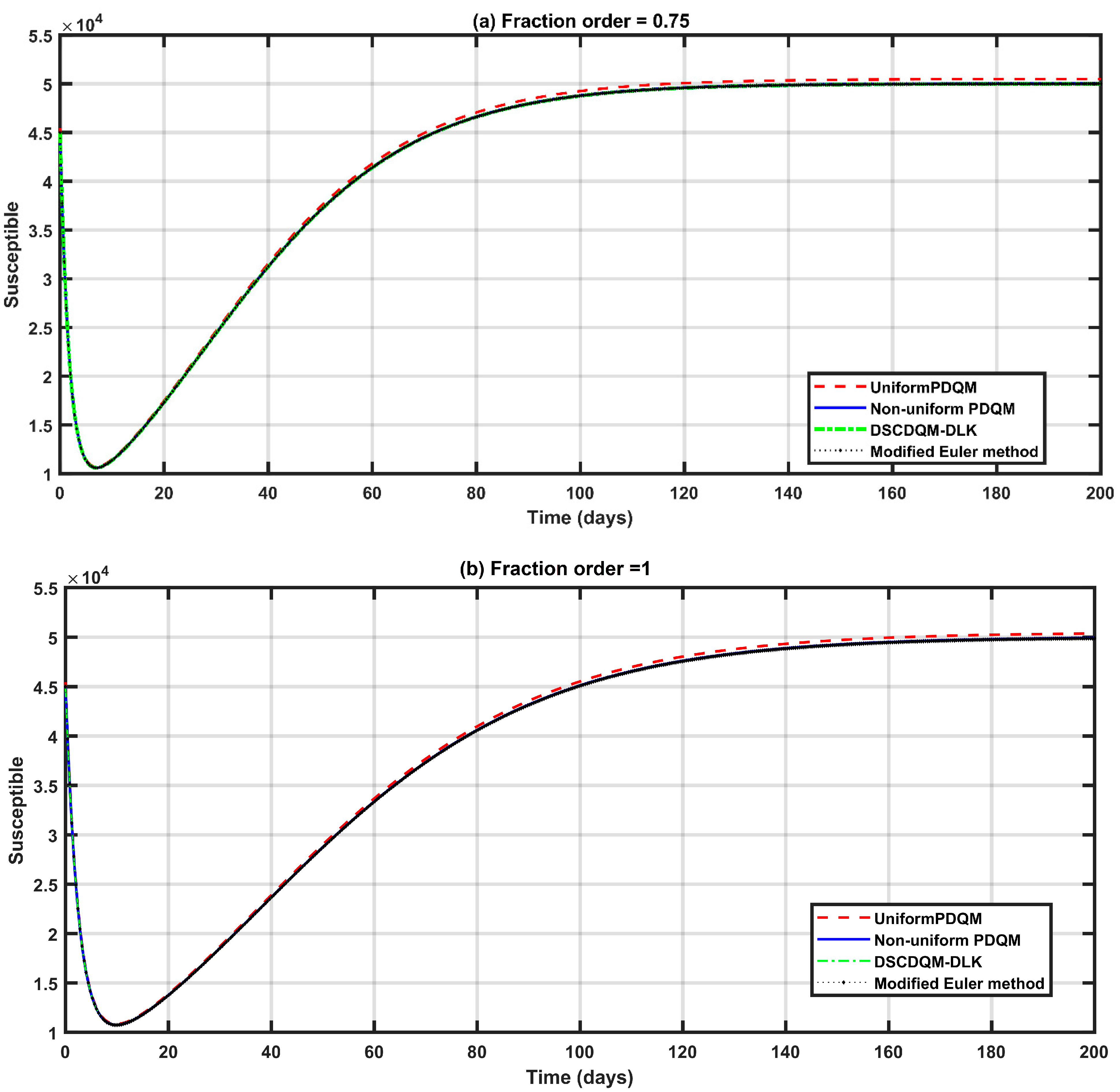
4. Numerical Results and Discussion

In the present paper, the MATLAB code was designed for computations and graphs. The configuration of the computer used to perform the simulation results was HP Probook 450 G8 Laptop-11th Intel Core i5-1135G7, 8 GB RAM, 512 GB PCIe NVMe SSD, 15.6″ FHD (1920 × 1080), Intel Iris X Graphics. This code was used to investigate the dynamics of COVID-19 infection and transmission. The validity, efficiency, and accuracy of the developed techniques were compared to the computed results of previous numerical and analytical solutions [11,28]. To assess the convergence and accuracy of the developed methods, the error-computation method outlined in [29,30] was used:

$$L_{\infty }Error=\underset{1\le i\le N}{max}\left|{\upsilon }_{numerical}\left(t_i\right)-{\upsilon }_{exact}\left(t_i\right)\right|,$$

(21)

The COVID-19 mathematical model was introduced as an algebraic system after substituting Equations (18) and (19) for the proposed methods in the system (1)–(6), as follows:

$$\begin{gathered} {\displaystyle \sum }_{j=1}^N{\Re }_{ij}^{\eta }{S}_p\left(t_j\right)={\mathsf{\Lambda }}_p-m_p{\displaystyle \sum }_{j=1}^N{\delta }_{ij}{S}_p\left(t_j\right)-{\beta }_p{\displaystyle \sum }_{j=1}^N{\delta }_{ij}{S}_p\left(t_j\right)\left({\displaystyle \sum }_{j=1}^N{\delta }_{ij}{I}_p\left(t_j\right)+k{\displaystyle \sum }_{j=1}^N{\delta }_{ij}{A}_p\left(t_j\right)\right) \\ -{\beta }_W{\displaystyle \sum }_{j=1}^N{\delta }_{ij}{S}_p\left(t_j\right){\displaystyle \sum }_{j=1}^N{\delta }_{ij}{S}_p\left(t_j\right), \end{gathered}$$

(22)

$$\begin{gathered} {\displaystyle \sum }_{j=1}^N{\Re }_{ij}^{\eta }{E}_p\left(t_j\right)={\beta }_p{\displaystyle \sum }_{j=1}^N{\delta }_{ij}{S}_p\left(t_j\right)\left({\displaystyle \sum }_{j=1}^N{\delta }_{ij}{I}_p\left(t_j\right)+k{\displaystyle \sum }_{j=1}^N{\delta }_{ij}{A}_p\left(t_j\right)\right)+{\beta }_W{\displaystyle \sum }_{j=1}^N{\delta }_{ij}{S}_p\left(t_j\right){\displaystyle \sum }_{j=1}^N{\delta }_{ij}{W}_p\left(t_j\right) \\ -\left[\left(1-{\delta }_p\right){\omega }_p{\displaystyle \sum }_{j=1}^N{\delta }_{ij}{E}_p\left(t_j\right)+{\delta }_p{\acute{\omega }}_p{\displaystyle \sum }_{j=1}^N{\delta }_{ij}{E}_p\left(t_j\right)+m_p\right]{\displaystyle \sum }_{j=1}^N{\delta }_{ij}{E}_p\left(t_j\right), \end{gathered}$$

(23)

$${\displaystyle \sum }_{j=1}^N{\Re }_{ij}^{\eta }{I}_p\left(t_j\right)=\left(1-{\delta }_p\right){\omega }_p{\displaystyle \sum }_{j=1}^N{\delta }_{ij}{E}_p\left(t_j\right)-\left({\gamma }_p+m_p\right){\displaystyle \sum }_{j=1}^N{\delta }_{ij}{I}_p\left(t_j\right),$$

(24)

$${\displaystyle \sum }_{j=1}^N{\Re }_{ij}^{\eta }{A}_p\left(t_j\right)={\delta }_p{\acute{\omega }}_p{\displaystyle \sum }_{j=1}^N{\delta }_{ij}{E}_p\left(t_j\right)-\left({\acute{\gamma }}_p+m_p\right){\displaystyle \sum }_{j=1}^N{\delta }_{ij}{A}_p\left(t_j\right),$$

(25)

$${\displaystyle \sum }_{j=1}^N{\Re }_{ij}^{\eta }{R}_p\left(t_j\right)={\gamma }_p{\displaystyle \sum }_{j=1}^N{\delta }_{ij}{I}_p\left(t_j\right)+{\acute{\gamma }}_p{\displaystyle \sum }_{j=1}^N{\delta }_{ij}{A}_p\left(t_j\right)-m_p{\displaystyle \sum }_{j=1}^N{\delta }_{ij}{R}_p\left(t_j\right),$$

(26)

$${\displaystyle \sum }_{j=1}^N{\Re }_{ij}^{\eta }{W}_p\left(t_j\right)={\mu }_p{\displaystyle \sum }_{j=1}^N{\delta }_{ij}{I}_p\left(t_j\right)+{\acute{\mu }}_p{\displaystyle \sum }_{j=1}^N{\delta }_{ij}{A}_p\left(t_j\right)-\epsilon {\displaystyle \sum }_{j=1}^N{\delta }_{ij}{W}_p\left(t_j\right),$$

(27)

Moreover, to deal with the initial conditions (7), this was performed by adapting the governing Equations (22)–(27).

Here, we chose some appropriate values for the parameters used in the model that is provided in

Table 1. Description of the parameters involved in the model.

Parameters	Description of Parameters
$S_p=\mathrm{800,000}$	Susceptible people
$E_p=\mathrm{200,000}$	Exposed people
$I_p=200$	Infected people
$A_p=250$	Asymptomatic people
$R_p=0$	Recovered people
$W=\mathrm{50,000}$	Resivior
$m_p=0.1$	Rate of death
${\mathsf{\Lambda }}_p=n_p\times N_p=5000$	Total population and birth rate
${\omega }_p=0.01$	Incubation period
${\acute{\omega }}_p=0.768$	Latent period
${\gamma }_p=1.05$	Infectious period of symptomatic infection
${\acute{\gamma }}_p=0.00001$	Infectious period of asymptomatic infection of people
${\beta }_p=0.00006$	Transmission rate from $I_p$ to $S_p$

(see [31]).

4.1. Validation of the DQM

To validate the current method, the DQM, the results of the uniform PDQM, the non-uniform PDQM, and DSCDQM-DLK were compared to a modified Euler method [11]. The comparisons are depicted in Figure 1a,b.

Moreover, the numerical results were tabulated, as shown in

Table 2. Computation of errors of infected people via uniform and non-uniform PDQM at different grid points (N) and fractional orders ($\eta$) for $t=100$ days, compared to Nazir et al. [11].

N	Uniform PDQM				Non-Uniform PDQM
	$\mathit{\eta }=0.5$	$\mathit{\eta }=0.7$	$\mathit{\eta }=0.85$	$\mathit{\eta }=1$	$\mathit{\eta }=0.5$	$\mathit{\eta }=0.7$	$\mathit{\eta }=0.85$	$\mathit{\eta }=1$
100	0.00485996	0.12370351	0.81045132	3.66075705	0.00102353	0.06231845	0.61910253	3.65824812
150	0.00218186	0.08663727	0.70389814	3.65692309	2.507 × 10−4	3.436 × 10−2	0.49322681	3.65322267
200	4.984 × 10−4	0.04583646	0.55019547	3.65296345	6.885 × 10−5	0.02023349	0.40486598	3.64996646
250	1.297 × 10−4	0.02617926	0.44544264	3.65013186	3.737 × 10−5	0.01583587	0.37004211	3.64968175
300	3.737 × 10−5	0.01583587	0.37004211	3.64968174	2.069 × 10−5	0.01253342	0.33987774	3.64941908
350	2.069 × 10−5	0.01253338	0.33987770	3.64941911	2.069 × 10−5	0.01253332	0.33987764	3.64941908
400	2.069 × 10−5	0.01253332	0.33987764	3.64941908	2.069 × 10−5	0.01253332	0.33987764	3.64941908
Nazir et al. [11]	2.069 × 10−5	0.01253332	0.33987764	3.64941908	2.069 × 10−5	0.01253332	0.33987764	3.64941908
Execution time	1.75 (second)–uniform $N\ge 350$				1.013 (second)–non-uniform N ≥ 300

,

Table 3. Computation of errors of infected people via uniform and non-uniform PDQM at different times (days) and fractional orders, compared to Nazir et al. [11].

Time (Days)	Uniform PDQM				Non-Uniform PDQM
	$\mathit{\eta }=0.5$	$\mathit{\eta }=0.7$	$\mathit{\eta }=0.85$	$\mathit{\eta }=1$	$\mathit{\eta }=0.5$	$\mathit{\eta }=0.7$	$\mathit{\eta }=0.85$	$\mathit{\eta }=1$
50	0.0788283	3.63412536	22.296806	73.305437	0.0788282	3.63412535	22.296805	73.305437
100	2.069 × 10−5	0.01253332	0.33987764	3.64941908	2.069 × 10−5	0.01253332	0.33987764	3.64941908
150	3.652 × 10−5	0.00185976	0.0198937	0.1422236	3.652 × 10−5	0.00185975	0.0198932	0.1422236
200	2.213 × 10−6	7.790 × 10−5	7.474 × 10−4	0.0053206	2.213 × 10−6	7.790 × 10−5	7.474 × 10−4	0.0053206
250	1.886 × 10−7	4.121 × 10−6	3.164 × 10−5	1.973 × 10−4	1.886 × 10−7	4.121 × 10−6	3.164 × 10−5	1.973 × 10−4
300	2.053 × 10−8	2.597 × 10−7	1.470 × 10−6	7.287 × 10−6	2.053 × 10−8	2.597 × 10−7	1.470 × 10−6	7.287 × 10−6
350	2.692 × 10−9	1.881 × 10−8	7.369 × 10−8	2.680 × 10−7	2.692 × 10−9	1.881 × 10−8	7.369 × 10−8	2.680 × 10−7
Execution time	1.75 (second)–uniform $N\ge 350$				1.0 (second)–non-uniform $N\ge 300$

and

Table 4. Computation of errors of infected people via DSCDQM-DLK at different grid points (N) and fractional orders ($\eta$) for $t=200$ days, compared to Nazir et al. [11].

N	Non-Uniform PDQM				DSCDQM-DLK
	$\mathit{\eta }=0.5$	$\mathit{\eta }=0.7$	$\mathit{\eta }=0.85$	$\mathit{\eta }=1$	$\mathit{\eta }=0.5$	$\mathit{\eta }=0.7$	$\mathit{\eta }=0.85$	$\mathit{\eta }=1$
100	1.977 × 10−5	0.813 × 10−4	1.717 × 10−3	0.0134789	2.405 × 10−6	8.321 × 10−5	7.874 × 10−4	0.0061135
150	0.155 × 10−5	0.344 × 10−4	0.265 × 10−3	0.0102579	2.354 × 10−6	7.925 × 10−5	7.659 × 10−4	0.0057321
200	2.632 × 10−6	8.001 × 10−5	7.913 × 10−4	0.0065217	2.213 × 10−6	7.790 × 10−5	7.474 × 10−4	0.0053206
250	2.401 × 10−6	7.877 × 10−5	7.725 × 10−4	0.0060214	2.213 × 10−6	7.790 × 10−5	7.474 × 10−4	0.0053206
300	2.213 × 10−6	7.790 × 10−5	7.474 × 10−4	0.0053206	2.213 × 10−6	7.790 × 10−5	7.474 × 10−4	0.0053206
350	2.213 × 10−6	7.790 × 10−5	7.474 × 10−4	0.0053206	2.213 × 10−6	7.790 × 10−5	7.474 × 10−4	0.0053206
400	2.213 × 10−6	7.790 × 10−5	7.474 × 10−4	0.0053206	2.213 × 10−6	7.790 × 10−5	7.474 × 10−4	0.0053206
Nazir et al. [11]	2.213 × 10−6	7.790 × 10−5	7.474 × 10−4	0.0053206	2.213 × 10−6	7.790 × 10−5	7.474 × 10−4	0.0053206
Execution time	1.025 (second)–non-uniform $N\ge 300$				0.5 (second)–non-uniform $N\ge 200$

, and compared to those of [11], including the execution time of the code. The proposed methods were applied to solve fractional differential equations, which could provide a more accurate representation of the dynamics of COVID-19. Fractional differential equations capture memory effects and long-range interactions, which can be relevant in modeling infectious diseases. Figure 1a,b and Table 2, Table 3 and Table 4 show substantial agreement with previous work, but with better execution times. Therefore, the PDQM and the DSCDQM have high accuracy and convergence when solving fractional differential equations. By using appropriate grid points and weighting functions, these methods can provide accurate approximations of the solution. The results are comparable with recent research [28,32].

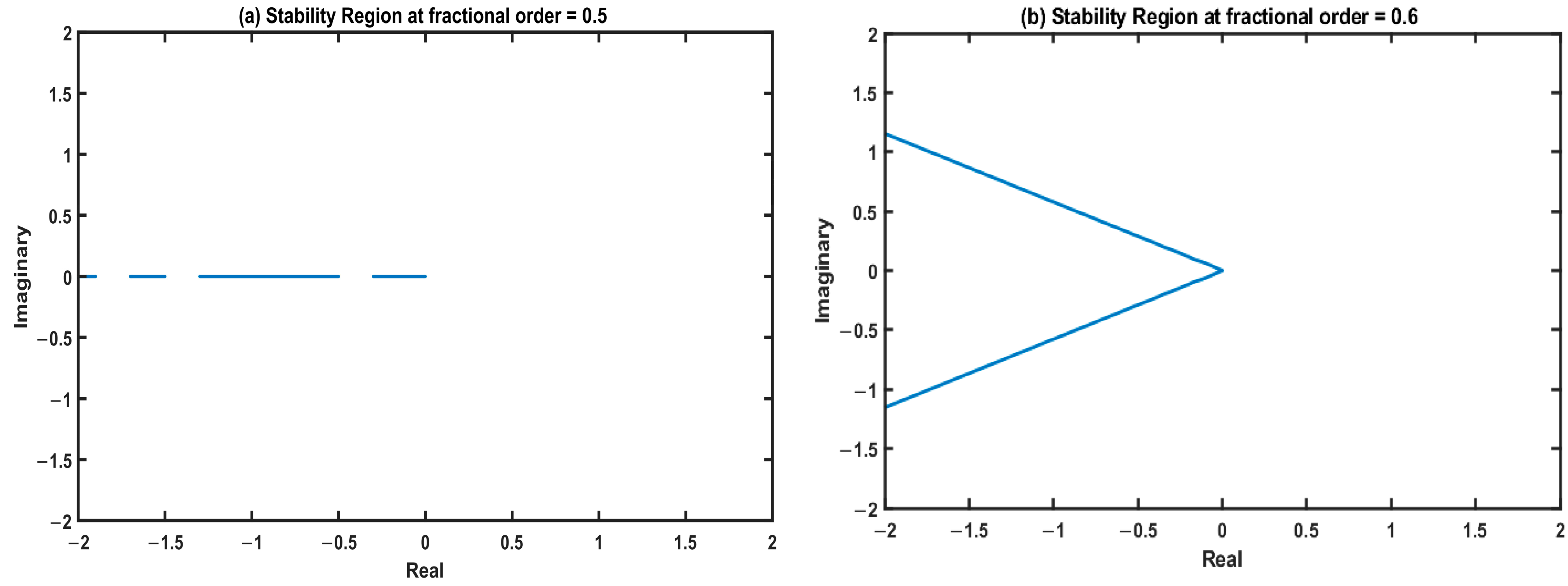
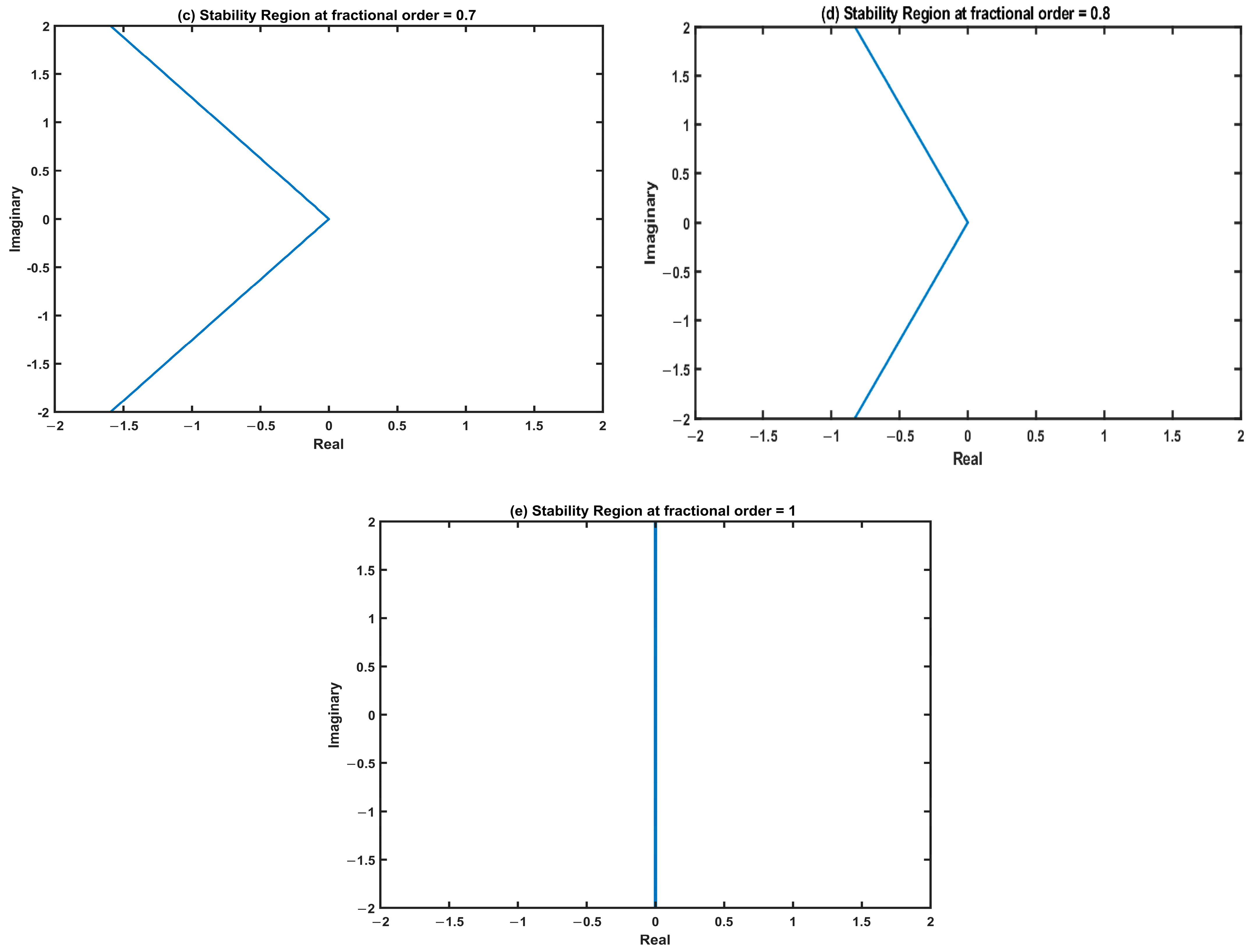
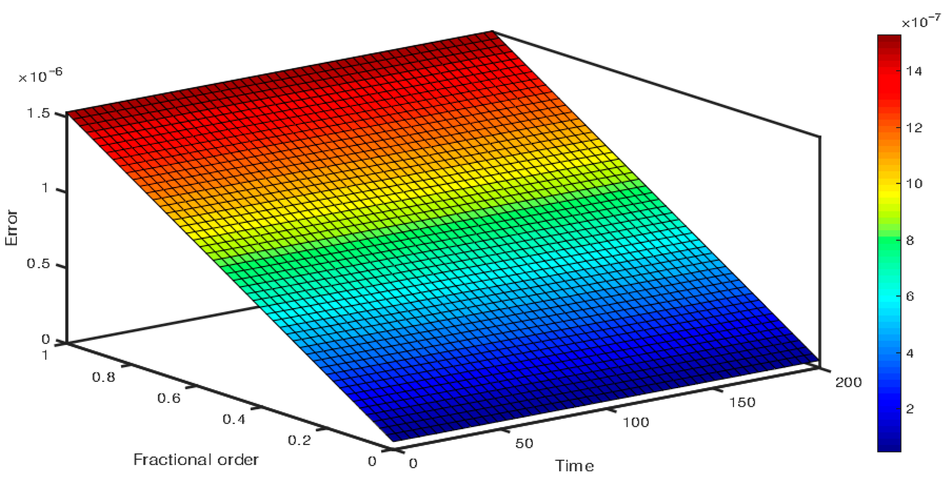
4.2. Stability Analysis

After a discretization process using the proposed schemes, a set of ordinary differential equations in time was obtained as an alternative to Equations (1)–(6) in the following form:

$$\frac{\mathrm{d}\left[U\right]}{\mathrm{dt}}=\mathrm{R}\left[U\right]+\left[\mathrm{K}\right]$$

(28)

where

• $\left\{U\right\}={\left({\mathrm{S}}_{\mathrm{p}},{\mathrm{E}}_{\mathrm{p}},{\mathrm{I}}_{\mathrm{p}},{\mathrm{A}}_{\mathrm{p}},{\mathrm{R}}_{\mathrm{p}},\mathrm{W}\right)}^{\mathrm{T}}$ are the unknown variables at the internal nodes of the grid;
• $\left[\mathrm{K}\right]$ is a vector including the initial conditions;
• $\mathrm{R}\left[U\right]$ represents the right-hand side of Equations (22)–(27); and
• ${\Re }_{ij}^{\left(1\right)}$ is the matrix of the weighting coefficient:

$${\Re }_{ij}^{\left(1\right)}={\left[\begin{array}{ccc}\begin{array}{cc}{\Re }_{22}^{\left(1\right)}& {\Re }_{23}^{\left(1\right)}\\ {\Re }_{32}^{\left(1\right)}& {\Re }_{33}^{\left(1\right)}\end{array}& \cdots & \begin{array}{c}{\Re }_{2\left(n-1\right)}^{\left(1\right)}\\ {\Re }_{3\left(n-1\right)}^{\left(1\right)}\end{array}\\ ⋮& \ddots & ⋮\\ \begin{array}{cc}{\Re }_{\left(n-1\right)2}^{\left(1\right)}& {\Re }_{\left(n-1\right)3}^{\left(1\right)}\end{array}& \cdots & {\Re }_{\left(n-1\right)\left(n-1\right)}^{\left(1\right)}\end{array}\right]}_{\left(N-2\right)\times \left(N-2\right)}$$

(29)

Based on the stability of the system (28), the stability of the suggested technique was examined. The bases of the stability analysis were the Eigen values of the coefficient matrices $“\Re$”. If the real part of each Eigen value of $“\Re ”$ was either negative or zero, one can conclude that the system (28) would be stable. This is illustrated by Figure 2. Moreover, the error propagation with respect to time and fractional order is depicted in Figure 3.

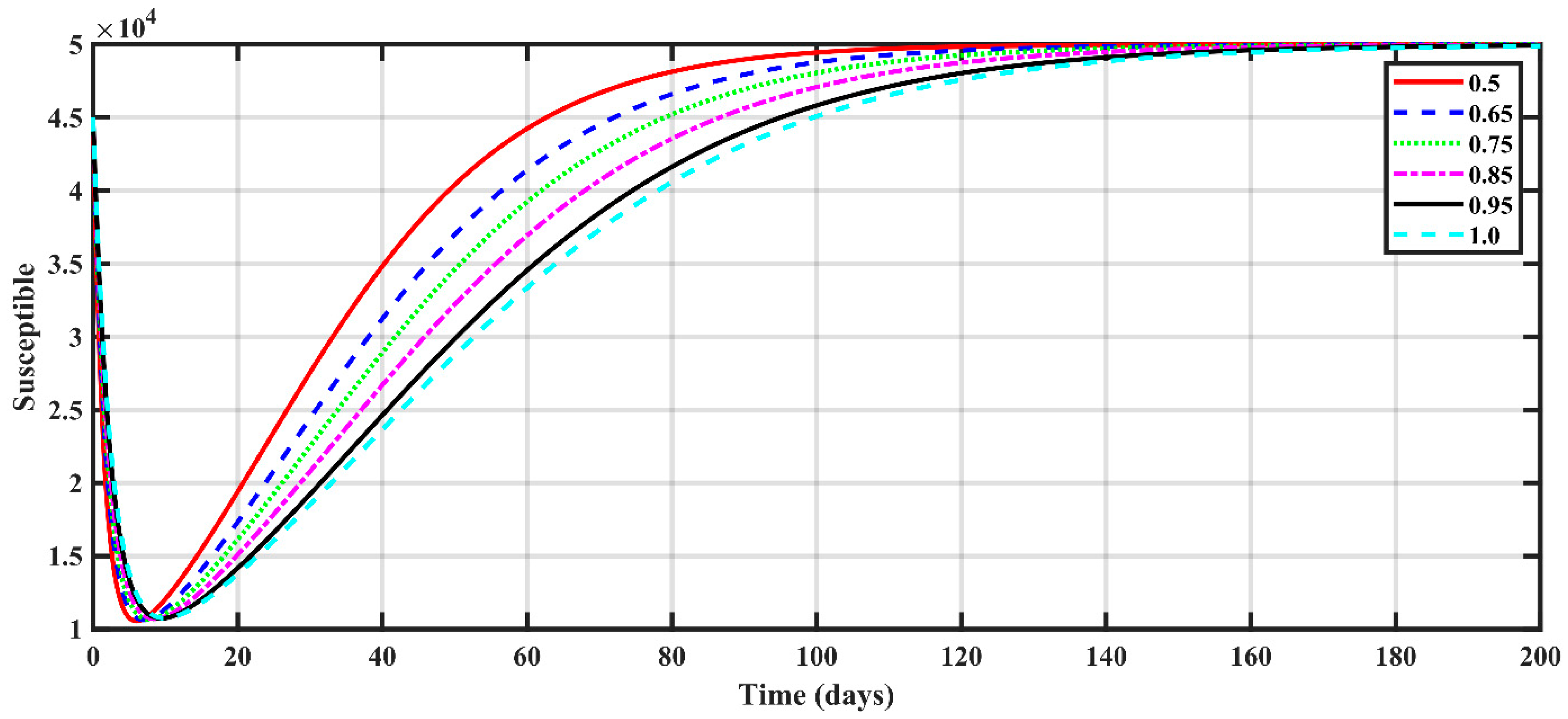
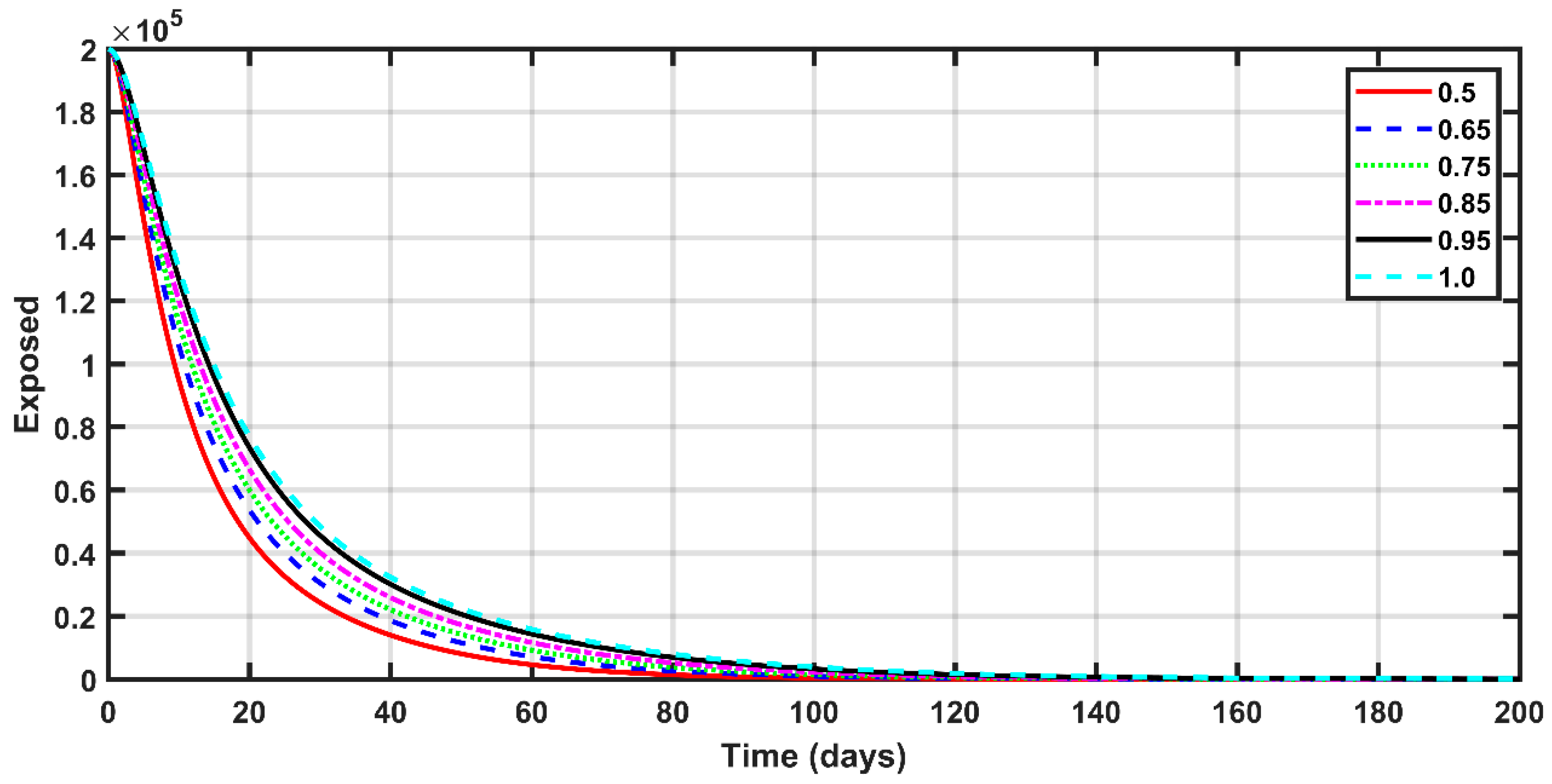
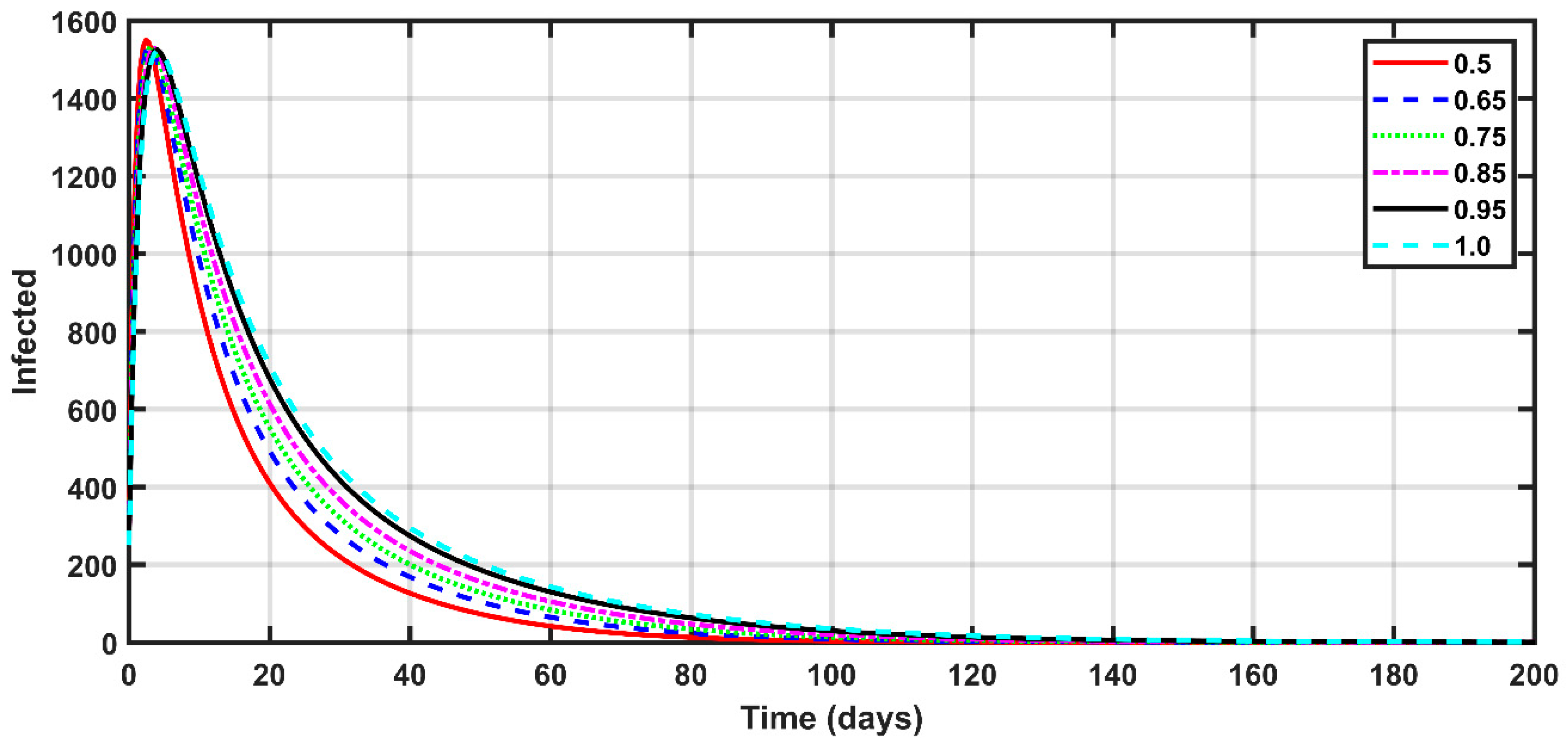
4.3. COVID-19 Dynamics

The graphical representation in Figure 4 illustrates the variation of the susceptible population over time, considering different fractional orders: η = 0.5, 0.65, 0.75, 0.85, 0.95, and 1. The results indicated a decreasing trend in the susceptible number of people as the fractional order increased. Initially, the susceptible count experienced a significant decline within the first month. Subsequently, it rose until it reached its maximum value after a period that depended on the specific fractional order. Notably, when the fractional order was small, the susceptible population peaked earlier than it did with higher fractional orders. As shown in Figure 5, there was a decrease in the number of exposed individuals over time, particularly when a smaller fractional order was employed. In such cases, the exposed population diminished rapidly and quickly vanished. Figure 6 provides insights into the behavior of the infected population. It demonstrates that there was a substantial increase in the number of infected individuals during the initial week of the investigation, primarily due to the high rate of disease transmission. Consequently, the number of recovered individuals, as depicted in Figure 7, displayed an increasing trend when the number of infected individuals was high. However, the count of recoveries eventually decreased due to continuous medical care, which aided in reducing the number of infected patients. On a related note, the implementation of rigorous medical care and home quarantine procedures enabled medical staff to effectively reduce the number of deaths resulting from COVID-19 infection. This decline is clearly illustrated in Figure 8. Furthermore, Figure 9 highlights the rapid decline in asymptomatic individuals within the first three months of infection.

Additionally, as shown in Figure 4, Figure 5, Figure 6, Figure 7, Figure 8 and Figure 9, the considered model depends on the order and offers more flexibility. As we increased the values of $\eta$, we saw that the solution tended to be in integer-order solution. The growing and decaying rates of various model classes differed in different fractional orders. Therefore, fractional calculus helped in understanding the transmission dynamics of COVID-19. In a smaller fractional order, the decay process was faster while the growth rate was slower. Increasing the fractional order may have slowed the decay process while the growth rate increased.

Moreover, the fractional order had a great impact on the transmission dynamics of the proposed model. In addition, it helped in better understanding the physical behavior of a spreading infection in a community. Moreover, the adopted numerical methods can be used as a fruitful technique to achieve computational results for such nonlinear problems. Various compartments’ concerned growth or decay processes were slightly faster at lower fractional orders, compared to the greater value of $\eta$. These graphical representations provide valuable insights into the dynamics of various population groups during infection. The analysis demonstrates the impact of fractional order on the susceptible, exposed, infected, recovered, deceased, and asymptomatic populations. These findings contribute to a deeper understanding of COVID-19’s progression and can aid in formulating effective strategies for disease management and control.

The relationship between the number of recovered individuals and the prevalence of infected individuals provides valuable insights into the trajectory of a pandemic such as COVID-19. Understanding this relationship helps assess the disease’s progression, estimate the effectiveness of control measures, and predict future trends. Here are some key observations:

As shown in Figure 6, Figure 7 and Figure 8, the number of recovered individuals directly impacts the prevalence of infected individuals. As more individuals recover, the pool of susceptible individuals decreases, leading to a decline in virus transmission. This reduction helps slow the spread of the disease and reduces the overall prevalence of infected individuals over time. The relationship between recovered and infected individuals is closely linked to herd immunity. When a significant portion of the population becomes immune through infection or vaccination, it creates a protective barrier that limits the transmission of the disease. This reduces the prevalence of infected individuals and helps to control the pandemic. By closely monitoring the relationship between the number of recovered and infected individuals, public health officials and policymakers can gain insights into the trajectory of the pandemic. They can assess the effectiveness of interventions, make informed decisions regarding control measures, and predict future trends in disease transmission. This understanding helps in the management of healthcare resources, the planning of vaccination campaigns, and the implementation of targeted measures to mitigate the impact of the pandemic.

5. Conclusions

The numerical solution for the mathematical model (1–6) that captures the dynamics of COVID-19 was achieved by utilizing two techniques within the differential quadrature method. The first technique employed was the polynomial-based differential quadrature method (PDQM), available in uniform and non-uniform cases. The second technique used was the discrete singular convolution (DSCDQM). Caputo’s fractional derivatives describe the fractional derivatives within the model. Several conclusions were established through the implementation of these techniques and fractional derivatives, contributing to a deeper understanding of the dynamics of COVID-19. The following key conclusions were drawn:

• The used techniques—uniform PDQM, non-uniform PDQM, and DSCDQM—showed higher accuracy than the modified Euler method [11], with better execution times.
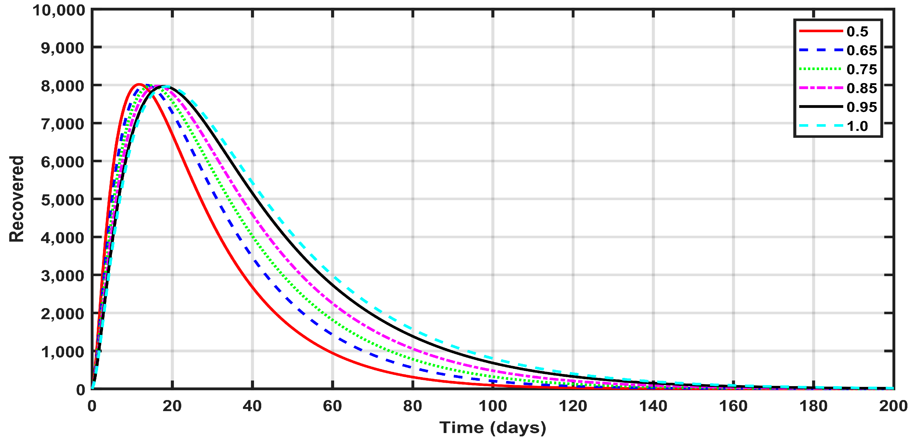
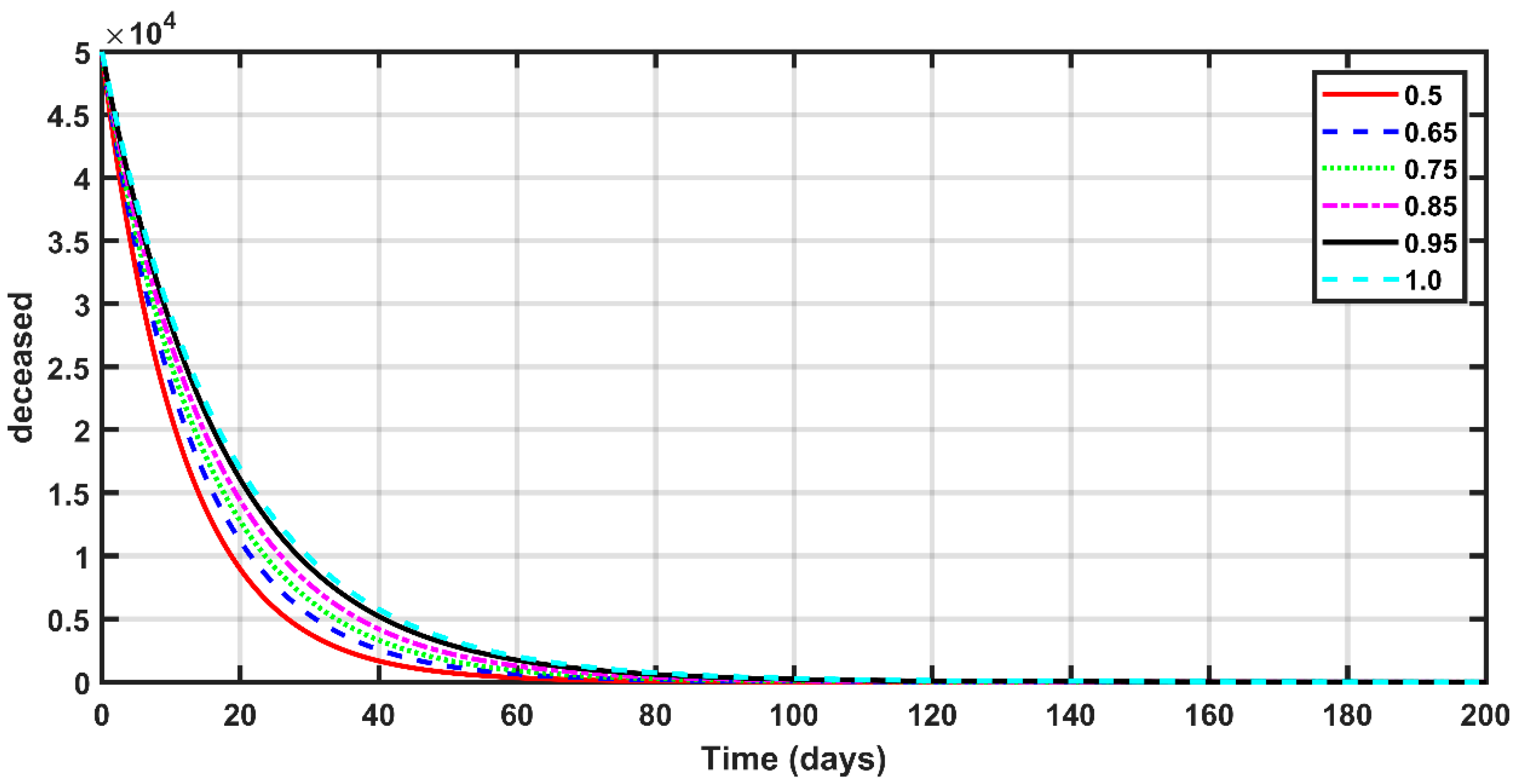
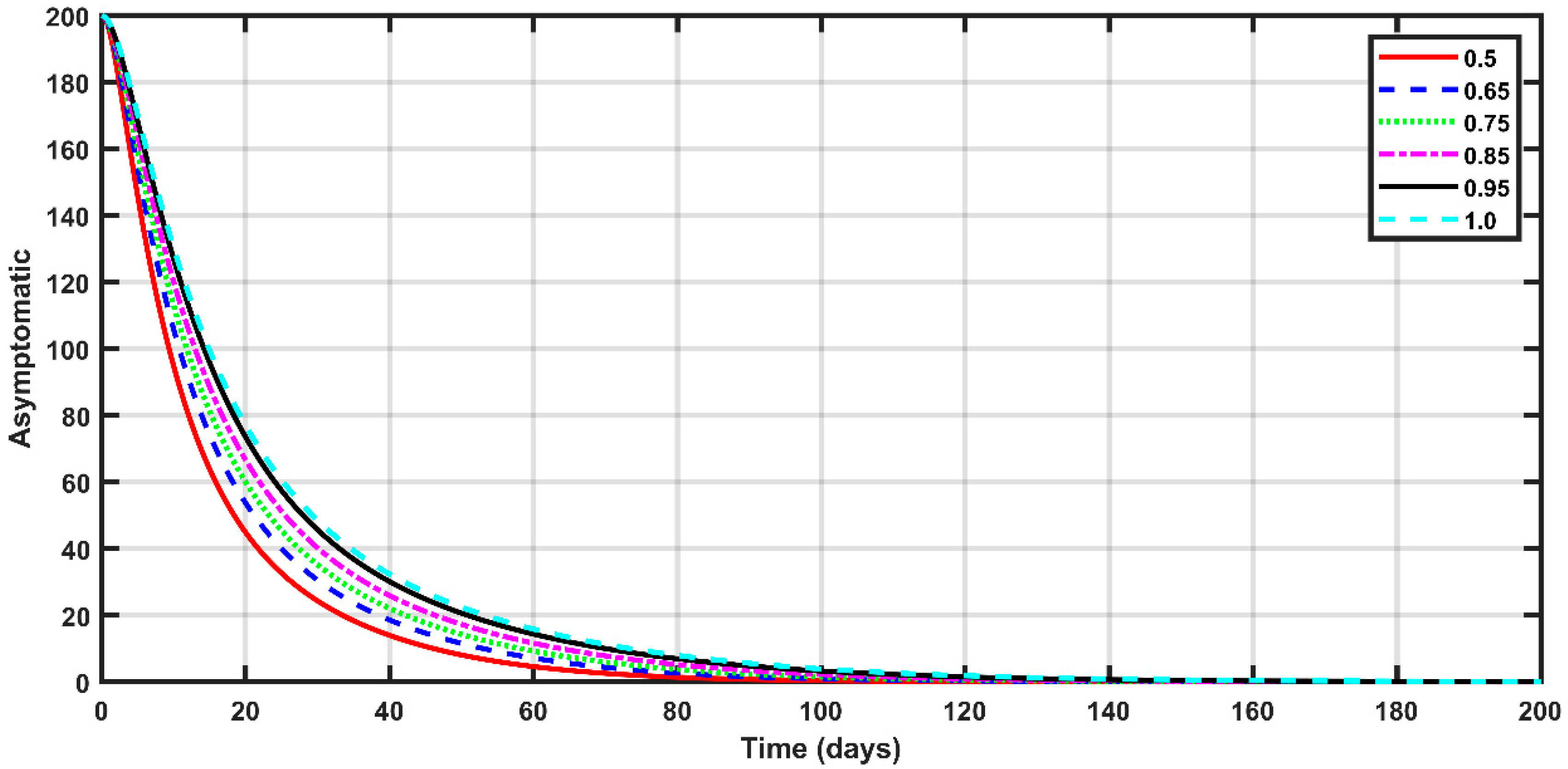
• The fractional order had a great impact on the results. As the fractional order approached one, the expected numbers of susceptible, exposed, deceased, asymptomatic, and recovered people became larger.
• The rise in the number of susceptible people was dramatic in the first month, then increased until it reached maximum values after a period, depending on the fractional order.
• The number of infected people increased significantly in the first week of the investigation, due to the high-spread rate of the disease. Consequently, the number of recovered people increased during the period with the higher number of infected people.
• The number of recovered people decreased due to the continuing medical care, which decreased the number of infected patients.

These conclusions provide valuable insights into the behavior and dynamics of COVID-19, shedding light on the patterns observed in different population groups. The numerical solutions obtained through the differential quadrature methods offer a comprehensive understanding of the pandemic’s progression and aid in formulating effective disease-control and management strategies. Moreover, the employed techniques demonstrated their superiority over the modified Euler method in both accuracy and execution time. The result highlights the practicality and reliability of the polynomial-based differential quadrature method (both uniform and non-uniform cases) and the discrete singular convolution method for simulating the dynamics of COVID-19. Overall, the numerical solutions and the conclusions contribute to the scientific understanding of the pandemic, providing valuable information for policymakers, healthcare professionals, and researchers working toward mitigating the impact of COVID-19.

References

1. Rezaei, N. Coronavirus Disease—COVID-19; Springer: Cham, Switzerland, 2021. [Google Scholar]
2. Murphy, P. COVID-19: Proportionality, Public Policy and Social Distancing; Palgrave Macmillan: Basingstoke, UK, 2020. [Google Scholar]
3. Chen, T.M.; Rui, J.; Wang, Q.P.; Zhao, Z.Y.; Cui, J.A.; Yin, L. A mathematical model for simulating the phase-based transmissibility of a novel coronavirus. Infect. Dis. Poverty 2020, 9, 24. [Google Scholar] [PubMed]
4. Kilbas, A.A.; Srivastava, H.M.; Trujillo, J.J. Theory and Applications of Fractional Differential Equations, 1st ed.; Elsevier: Amsterdam, The Netherlands, 2006. [Google Scholar]
5. Lakshmikantham, V.; Leela, S.; Vasundhara Devi, J. Theory of Fractional Dynamic Systems; CSP: Cambridge, UK, 2009. [Google Scholar]
6. Mathai, A.M.; Haubold, H.J. An Introduction to Fractional Calculus; Nova Science Publishers: Hauppauge, NY, USA, 2017. [Google Scholar]
7. Singh, J.; Hristov, J.Y.; Hammouch, Z. New Trends in Fractional Differential Equations with Real-World Applications in Physics; Frontiers Media SA: Lausanne, Switzerland, 2020. [Google Scholar]
8. Yasmin, H.; Aljahdaly, N.H.; Saeed, A.M.; Shah, R. Probing Families of Optical Soliton Solutions in Fractional Perturbed Radhakrishnan–Kundu–Lakshmanan Model with Improved Versions of Extended Direct Algebraic Method. Fractal Fract. 2023, 7, 512. [Google Scholar]
9. Yasmin, H.; Aljahdaly, N.H.; Saeed, A.M.; Shah, R. Investigating Families of Soliton Solutions for the Complex Structured Coupled Fractional Biswas—Arshed Model in Birefringent Fibers Using a Novel Analytical Technique. Fractal Fract. 2023, 7, 491. [Google Scholar] [CrossRef]
10. Naeem, M.; Yasmin, H.; Shah, R.; Shah, N.A.; Nonlaopon, K. Investigation of Fractional Nonlinear Regularized Long-Wave Models via Novel Techniques. Symmetry 2023, 15, 220. [Google Scholar] [CrossRef]
11. Nazir, G.; Zeb, A.; Shah, K.; Saeed, T.; Khan, R.A.; Khan, S.I.U. Study of COVID-19 mathematical model of fractional order via modified Euler method. Alex. Eng. J. 2021, 60, 5287–5296. [Google Scholar] [CrossRef]
12. Mpinganzima, L.; Ntaganda, J.M.; Banzi, W.; Muhirwa, J.P.; Nannyonga, B.K.; Niyobuhungiro, J.; Rutaganda, E. Analysis of COVID-19 mathematical model for predicting the impact of control measures in Rwanda. Inform. Med. Unlocked 2023, 37, 101195. [Google Scholar]
13. Mpinganzima, L.; Ntaganda, J.M.; Banzi, W.; Muhirwa, J.P.; Nannyonga, B.K.; Niyobuhungiro, J.; Rutaganda, E.; Ngaruye, I.; Ndanguza, D.; Nzabanita, J.; et al. Compartmental mathematical modelling of dynamic transmission of COVID-19 in Rwanda. IJID Reg. 2023, 6, 99–107. [Google Scholar]
14. Abioye, A.I.; Peter, O.J.; Ogunseye, H.A.; Oguntolu, F.A.; Ayoola, T.A.; Oladapo, A.O. A fractional-order mathematical model for malaria and COVID-19 co-infection dynamics. Heal. Anal. 2023, 4, 100210. [Google Scholar]
15. Alaje, A.I.; Olayiwola, M.O. A fractional-order mathematical model for examining the spatiotemporal spread of COVID-19 in the presence of vaccine distribution. Heal. Anal. 2023, 4, 100230. [Google Scholar]
16. Avusuglo, W.; Mosleh, R.; Ramaj, T.; Li, A.; Sharbayta, S.S.; Fall, A.A.; Ghimire, S.; Shi, F.; Lee, J.K.; Thommes, E.; et al. Workplace absenteeism due to COVID-19 and influenza across Canada: A mathematical model. J. Theor. Biol. 2023, 572, 111559. [Google Scholar]
17. Singh, R.; Rehman, A.U.; Ahmed, T.; Ahmad, K.; Mahajan, S.; Pandit, A.K.; Abualigah, L.; Gandomi, A.H. Mathematical modelling and analysis of COVID-19 and tuberculosis transmission dynamics. Inform. Med. Unlocked 2023, 38, 101235. [Google Scholar] [CrossRef]
18. Li, C.; Qian, D.; Chen, Y. On Riemann-Liouville and Caputo Derivatives. Discret. Dyn. Nat. Soc. 2011, 2011, 562494. [Google Scholar] [CrossRef]
19. Caputo, M. Linear Models of Dissipation whose Q is almost Frequency Independent—II. Geophys. J. Int. 1967, 13, 529–539. [Google Scholar] [CrossRef]
20. Zong, Z.; Zhang, Y. Advanced Differential Quadrature Methods; CRC Press: Boca Raton, FL, USA, 2009. [Google Scholar]
21. Shu, C. Differential Quadrature and Its Application in Engineering; Springer: London, UK, 2000. [Google Scholar]
22. Ragb, O.; Mohamed, M.; Matbuly, M. Vibration Analysis of Magneto-Electro-Thermo NanoBeam Resting on Nonlinear Elastic Foundation Using Sinc and Discrete Singular Convolution Differential Quadrature Method. Mod. Appl. Sci. 2019, 13, 49. [Google Scholar] [CrossRef]
23. Wei, G.W. Discrete singular convolution for the solution of the Fokker–Planck equation. J. Chem. Phys. 1999, 110, 8930–8942. [Google Scholar] [CrossRef]
24. Wan, D.C.; Zhou, Y.C.; Wei, G.W. Numerical solution of incompressible flows by discrete singular convolution. Int. J. Numer. Methods Fluids 2002, 38, 789–810. [Google Scholar] [CrossRef]
25. Zhang, L.; Xiang, Y.; Wei, G. Local adaptive differential quadrature for free vibration analysis of cylindrical shells with various boundary conditions. Int. J. Mech. Sci. 2006, 48, 1126–1138. [Google Scholar] [CrossRef]
26. Civalek, Ö.; Kiracioglu, O. Free vibration analysis of Timoshenko beams by DSC method. Int. J. Numer. Methods Biomed. Eng. 2010, 26, 1890–1898. [Google Scholar] [CrossRef]
27. Civalek, Ö. Free vibration of carbon nanotubes reinforced (CNTR) and functionally graded shells and plates based on FSDT via discrete singular convolution method. Compos. Part B Eng. 2017, 111, 45–59. [Google Scholar]
28. Ahmad, S.W.; Sarwar, M.; Shah, K.; Ahmadian, A.; Salahshour, S. Fractional order mathematical modeling of novel corona virus (COVID-19). Math. Methods Appl. Sci. 2021, 46, 7847–7860. [Google Scholar] [CrossRef]
29. Anley, E.F.; Zheng, Z. Finite Difference Method for Two-Sided Two Dimensional Space Fractional Convection-Diffusion Problem with Source Term. Mathematics 2020, 8, 1878. [Google Scholar] [CrossRef]
30. Dong, G.; Guo, Z.; Yao, W. Numerical methods for time-fractional convection-diffusion problems with high-order accuracy. Open Math. 2021, 19, 782–802. [Google Scholar]
31. Khan, M.A.; Atangana, A. Modeling the dynamics of novel coronavirus (2019-nCov) with fractional derivative. Alex. Eng. J. 2020, 59, 2379–2389. [Google Scholar] [CrossRef]
32. Yousif, R.; Jeribi, A.; Al-Azzawi, S. Fractional-Order SEIRD Model for Global COVID-19 Outbreak. Mathematics 2023, 11, 1036. [Google Scholar] [CrossRef]
Figure 1. (a,b) Comparison of different techniques of the DQM and a modified Euler method [11].
Computation 11 00198 g001
Figure 2. Stability regions at different fractional orders.
Computation 11 00198 g002aComputation 11 00198 g002b
Figure 3. Error propagation with respect to time and fractional order.
Computation 11 00198 g003
Figure 4. Susceptible people at different fractional orders.
Computation 11 00198 g004
Figure 5. Exposed people at different fractional orders.
Computation 11 00198 g005
Figure 6. Infected people at different fractional orders.
Computation 11 00198 g006
Figure 7. Recovered people at different fractional orders.
Computation 11 00198 g007
Figure 8. Deceased People at different fractional orders.
Computation 11 00198 g008
Figure 9. Asymptomatic people at different fractional orders.
Computation 11 00198 g009