
MLP-Mixer-Autoencoder: A Lightweight Ensemble Architecture for Malware Classification

Abstract
:1. Introduction
2. Related Work
2.1. CNN-Based Models
2.2. CNN-Free Models
3. Proposed Method
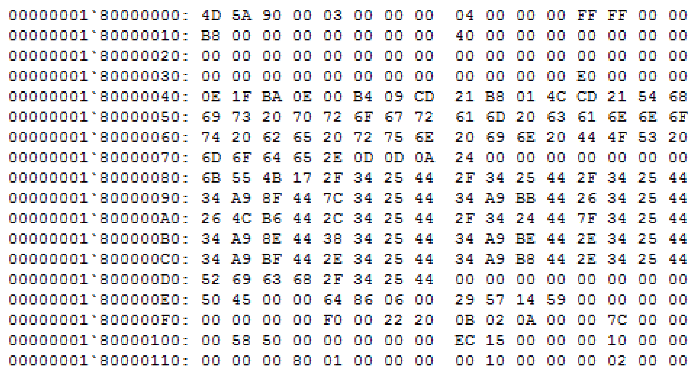
3.1. Image Representation for Malware
3.2. MLP-Mixer
3.3. Autoencoder
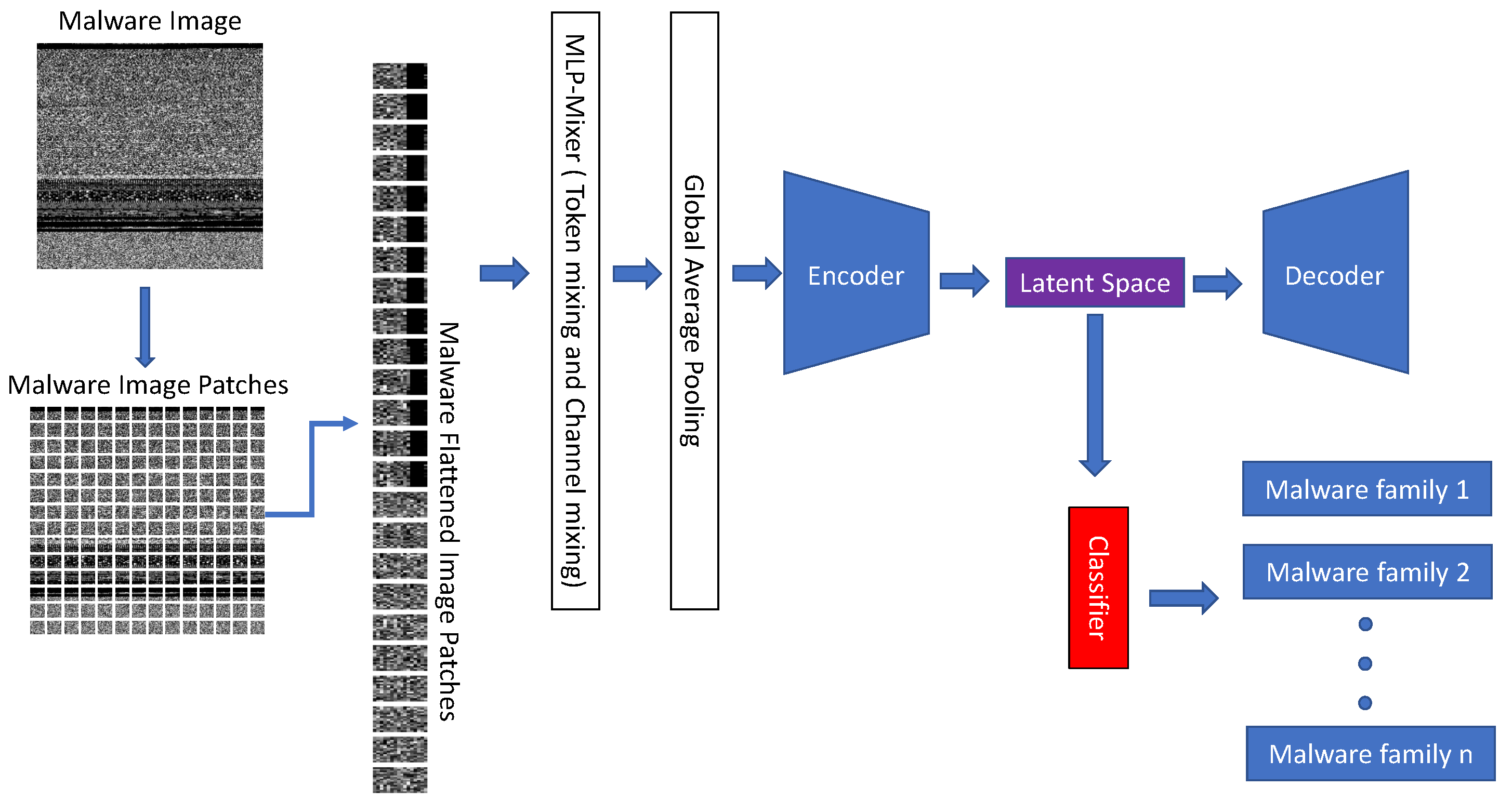
3.4. MLP-Mixer-AE
4. Experiments
4.1. Dataset
4.2. Evaluation Metrics
4.3. Evaluation Results and Discussion
5. Conclusions
Author Contributions
Funding
Data Availability Statement
Conflicts of Interest
References
- Malware Attacks Targeting Ukraine Government-Microsoft on the Issues. Available online: https://blogs.microsoft.com/on-the-issues/2022/01/15/mstic-malware-cyberattacks-ukraine-government/ (accessed on 14 December 2022).
- Malware Statistics & Trends Report|AV-TEST. Available online: https://www.av-test.org/en/statistics/malware (accessed on 14 December 2022).
- Raghuraman, C.; Suresh, S.; Shivshankar, S.; Chapaneri, R. Static and dynamic malware analysis using machine learning. In Proceedings of the First International Conference on Sustainable Technologies for Computational Intelligence, Jaipur, India, 29–30 March 2019; pp. 793–806. [Google Scholar]
- Ye, Y.; Li, T.; Adjeroh, D.; Iyengar, S.S. A survey on malware detection using data mining techniques. ACM Comput. Surv. (CSUR) 2017, 50, 1–40. [Google Scholar] [CrossRef]
- Belaoued, M.; Mazouzi, S. A chi-square-based decision for real-time malware detection using PE-file features. J. Inf. Process. Syst. 2016, 12, 644–660. [Google Scholar]
- Maulana, R.J.; Kusuma, G.P. Malware classification based on system call sequences using deep learning. Adv. Sci. Technol. Eng. Syst. J. 2020, 5, 207–216. [Google Scholar] [CrossRef]
- Demirkıran, F.; Çayır, A.; Ünal, U.; Dağ, H. An ensemble of pre-trained transformer models for imbalanced multiclass malware classification. Comput. Secur. 2022, 121, 102846. [Google Scholar] [CrossRef]
- Conti, G.; Dean, E.; Sinda, M.; Sangster, B. Visual reverse engineering of binary and data files. In Proceedings of the International Workshop on Visualization for Computer Security, Cambridge, MA, USA, 15 September 2008; pp. 1–17. [Google Scholar]
- Awan, M.J.; Masood, O.A.; Mohammed, M.A.; Yasin, A.; Zain, A.M.; Damaševičius, R.; Abdulkareem, K.H. Image-Based Malware Classification Using VGG19 Network and Spatial Convolutional Attention. Electronics 2021, 10, 2444. [Google Scholar] [CrossRef]
- Nataraj, L.; Karthikeyan, S.; Jacob, G.; Manjunath, B.S. Malware images: Visualization and automatic classification. In Proceedings of the 8th International Symposium on Visualization for Cyber Security, Pittsburgh, PA, USA, 20 July 2011; pp. 1–7. [Google Scholar]
- Rezende, E.; Ruppert, G.; Carvalho, T.; Ramos, F.; De Geus, P. Malicious software classification using transfer learning of resnet-50 deep neural network. In Proceedings of the 2017 16th IEEE International Conference on Machine Learning and Applications (ICMLA), Cancun, Mexico, 18–21 December 2017; pp. 1011–1014. [Google Scholar]
- Burks, R.; Islam, K.A.; Lu, Y.; Li, J. Data augmentation with generative models for improved malware detection: A comparative study. In Proceedings of the 2019 IEEE 10th Annual Ubiquitous Computing, Electronics & Mobile Communication Conference (UEMCON), New York City, NY, USA, 10–12 October 2019; pp. 0660–0665. [Google Scholar]
- Naeem, H.; Guo, B.; Ullah, F.; Naeem, M.R. A cross-platform malware variant classification based on image representation. KSII Trans. Internet Inf. Syst. (TIIS) 2019, 13, 3756–3777. [Google Scholar]
- Abijah Roseline, S.; Hari, G.; Geetha, S.; Krishnamurthy, R. Vision-based malware detection and classification using lightweight deep learning paradigm. In Proceedings of the International Conference on Computer Vision and Image Processing, Prayagraj, India, 4–6 December 2020; pp. 62–73. [Google Scholar]
- Nisa, M.; Shah, J.H.; Kanwal, S.; Raza, M.; Khan, M.A.; Damaševičius, R.; Blažauskas, T. Hybrid malware classification method using segmentation-based fractal texture analysis and deep convolution neural network features. Appl. Sci. 2020, 10, 4966. [Google Scholar] [CrossRef]
- Lee, J.; Lee, J. A Classification System for Visualized Malware Based on Multiple Autoencoder Models. IEEE Access 2021, 9, 144786–144795. [Google Scholar] [CrossRef]
- Hammad, B.T.; Jamil, N.; Ahmed, I.T.; Zain, Z.M.; Basheer, S. Robust Malware Family Classification Using Effective Features and Classifiers. Appl. Sci. 2022, 12, 7877. [Google Scholar] [CrossRef]
- Lin, W.C.; Yeh, Y.R. Efficient Malware Classification by Binary Sequences with One-Dimensional Convolutional Neural Networks. Mathematics 2022, 10, 608. [Google Scholar] [CrossRef]
- Barros, P.H.; Chagas, E.T.; Oliveira, L.B.; Queiroz, F.; Ramos, H.S. Malware-SMELL: A zero-shot learning strategy for detecting zero-day vulnerabilities. Comput. Secur. 2022, 120, 102785. [Google Scholar] [CrossRef]
- Wang, C.; Zhao, Z.; Wang, F.; Li, Q. MSAAM: A Multiscale Adaptive Attention Module for IoT Malware Detection and Family Classification. Secur. Commun. Netw. 2022. [Google Scholar] [CrossRef]
- Zhong, F.; Chen, Z.; Xu, M.; Zhang, G.; Yu, D.; Cheng, X. Malware-on-the-Brain: Illuminating Malware Byte Codes with Images for Malware Classification. IEEE Trans. Comput. 2022, 72, 438–451. [Google Scholar] [CrossRef]
- Son, T.T.; Lee, C.; Le-Minh, H.; Aslam, N.; Dat, V.C. An enhancement for image-based malware classification using machine learning with low dimension normalized input images. J. Inf. Secur. Appl. 2022, 69, 103308. [Google Scholar] [CrossRef]
- Falana, O.J.; Sodiya, A.S.; Onashoga, S.A.; Badmus, B.S. Mal-Detect: An intelligent visualization approach for malware detection. J. King Saud-Univ.-Comput. Inf. Sci. 2022, 34. [Google Scholar] [CrossRef]
- Ban, T.; Isawa, R.; Guo, S.; Inoue, D.; Nakao, K. Efficient malware packer identification using support vector machines with spectrum kernel. In Proceedings of the 2013 Eighth Asia Joint Conference on Information Security, Seoul, Korea, 25–26 July 2013; pp. 69–76. [Google Scholar]
- Wong, W.; Juwono, F.H.; Apriono, C. Vision-based malware detection: A transfer learning approach using optimal ECOC-SVM configuration. IEEE Access 2021, 9, 159262–159270. [Google Scholar] [CrossRef]
- Hemalatha, J.; Roseline, S.A.; Geetha, S.; Kadry, S.; Damaševičius, R. An efficient densenet-based deep learning model for malware detection. Entropy 2021, 23, 344. [Google Scholar] [CrossRef]
- Kim, H.M.; Lee, K.H. IIoT Malware Detection Using Edge Computing and Deep Learning for Cybersecurity in Smart Factories. Appl. Sci. 2022, 12, 7679. [Google Scholar] [CrossRef]
- Kumar, S. MCFT-CNN: Malware classification with fine-tune convolution neural networks using traditional and transfer learning in Internet of Things. Future Gener. Comput. Syst. 2021, 125, 334–351. [Google Scholar]
- Ding, Y.; Zhang, X.; Hu, J.; Xu, W. Android malware detection method based on bytecode image. J. Ambient. Intell. Humaniz. Comput. 2020, 1–10. [Google Scholar] [CrossRef]
- Bochinski, E.; Senst, T.; Sikora, T. Hyper-parameter optimization for convolutional neural network committees based on evolutionary algorithms. In Proceedings of the 2017 IEEE International Conference on Image Processing (ICIP), Beijing, China, 17–20 September 2017; pp. 3924–3928. [Google Scholar]
- Choi, S.; Bae, J.; Lee, C.; Kim, Y.; Kim, J. Attention-based automated feature extraction for malware analysis. Sensors 2020, 20, 2893. [Google Scholar] [CrossRef] [PubMed]
- Yakura, H.; Shinozaki, S.; Nishimura, R.; Oyama, Y.; Sakuma, J. Neural malware analysis with attention mechanism. Comput. Secur. 2019, 87, 101592. [Google Scholar] [CrossRef]
- Dosovitskiy, A.; Beyer, L.; Kolesnikov, A.; Weissenborn, D.; Zhai, X.; Unterthiner, T.; Dehghani, M.; Minderer, M.; Heigold, G.; Gelly, S.; et al. An image is worth 16x16 words: Transformers for image recognition at scale. arXiv 2010, arXiv:2010.11929. [Google Scholar]
- Tolstikhin, I.O.; Houlsby, N.; Kolesnikov, A.; Beyer, L.; Zhai, X.; Unterthiner, T.; Yung, J.; Steiner, A.; Keysers, D.; Uszkoreit, J.; et al. Mlp-mixer: An all-mlp architecture for vision. Adv. Neural Inf. Process. Syst. 2021, 34, 24261–24272. [Google Scholar]
- da Silva, A.A.; Pamplona Segundo, M. On Deceiving Malware Classification with Section Injection. Mach. Learn. Knowl. Extr. 2023, 5, 9. [Google Scholar] [CrossRef]
- Vu, D.L.; Nguyen, T.K.; Nguyen, T.V.; Nguyen, T.N.; Massacci, F.; Phung, P.H. HIT4Mal: Hybrid image transformation for malware classification. Trans. Emerg. Telecommun. Technol. 2020, 31, e3789. [Google Scholar] [CrossRef]
- Van Dao, T.; Sato, H.; Kubo, M. An Attention Mechanism for Combination of CNN and VAE for Image-Based Malware Classification. IEEE Access 2022, 10, 85127–85136. [Google Scholar]
- Liu, H.; Dai, Z.; So, D.; Le, Q.V. Pay attention to mlps. Adv. Neural Inf. Process. Syst. 2021, 34, 9204–9215. [Google Scholar]
- Rieck, K.; Trinius, P.; Willems, C.; Holz, T. Automatic analysis of malware behavior using machine learning. J. Comput. Secur. 2011, 19, 639–668. [Google Scholar] [CrossRef]
- Huang, W.C.; Di Troia, F.; Stamp, M. Robust Hashing for Image-based Malware Classification. In Proceedings of the ICETE, Porto, Portugal, 26–28 July 2018; pp. 617–625. [Google Scholar]
- Kim, S.; Jung, W.; Lee, K.; Oh, H.; Kim, E.T. Sumav: Fully automated malware labeling. ICT Express 2022, 8, 530–538. [Google Scholar] [CrossRef]
- Hurier, M.; Suarez-Tangil, G.; Dash, S.K.; Bissyandé, T.F.; Le Traon, Y.; Klein, J.; Cavallaro, L. Euphony: Harmonious unification of cacophonous anti-virus vendor labels for android malware. In Proceedings of the 2017 IEEE/ACM 14th International Conference on Mining Software Repositories (MSR), Buenos Aires, Argentina, 20–28 May 2017; pp. 425–435. [Google Scholar]
- Sebastián, S.; Caballero, J. Avclass2: Massive malware tag extraction from av labels. In Proceedings of the Annual Computer Security Applications Conference, Austin, TX, USA, 7–11 December 2020; pp. 42–53. [Google Scholar]
- Ghouti, L.; Imam, M. Malware classification using compact image features and multiclass support vector machines. IET Inf. Secur. 2020, 14, 419–429. [Google Scholar] [CrossRef]


| File Size | Image Height | Time Convert (ms) |
|---|---|---|
| <10 kB | 32 | 0.105 |
| 10 kB–30 kB | 64 | 0.312 |
| 30 kB–60 kB | 128 | 0.428 |
| 60 kB–100 kB | 256 | 0.571 |
| 100 kB–200 kB | 384 | 0.748 |
| 200 kB–500 kB | 512 | 0.665 |
| 500 kB–1 Mb | 768 | 0.814 |
| >1 Mb | 1024 | 2.85 |
| Class | Family Name | No. of Samples | Percentage (%) |
|---|---|---|---|
| 0 | Adialer.C | 122 | 1.31 |
| 1 | Agent.FYI | 116 | 2.12 |
| 2 | Allaple.A | 2949 | 31.58 |
| 3 | Appaple.L | 1591 | 17.04 |
| 4 | Alueron.gen!J | 198 | 2.12 |
| 5 | Autorun.K | 106 | 1.14 |
| 6 | C2LOP.gen!g | 200 | 2.14 |
| 7 | C2LOP.P | 146 | 1.56 |
| 8 | Dialplatform.B | 177 | 1.89 |
| 9 | Dontovo.A | 162 | 1.73 |
| 10 | Fakerean | 381 | 4.08 |
| 11 | Instantaccess | 431 | 4.62 |
| 12 | Lolyda.AA1 | 213 | 2.28 |
| 13 | Lolyda.AA2 | 184 | 1.97 |
| 14 | Lolyda.AA3 | 123 | 1.32 |
| 15 | Lolyda.AT | 159 | 1.70 |
| 16 | Malex.gen!J | 136 | 1.46 |
| 17 | Obfuscator.AD | 142 | 1.52 |
| 18 | Rbot!gen | 158 | 1.69 |
| 19 | Skintrim.N | 80 | 0.86 |
| 20 | Swizzor.gen!E | 128 | 1.37 |
| 21 | Swizzor.gen!I | 132 | 1.41 |
| 22 | VB.AT | 408 | 4.58 |
| 23 | Wintrim.BX | 97 | 1.04 |
| 24 | Yuner.A | 800 | 8.57 |
| Total | 9339 |
| Class | Family Name | No. of Samples | Percentage (%) |
|---|---|---|---|
| 0 | Adultbrowser | 262 | 8.36 |
| 1 | Allaple | 300 | 9.58 |
| 2 | Bancos | 48 | 1.53 |
| 3 | Casino | 140 | 4.47 |
| 4 | Dorfdo | 65 | 2.07 |
| 5 | Ejik | 168 | 5.36 |
| 6 | Flystudio | 33 | 1.05 |
| 7 | Ldpinch | 43 | 1.37 |
| 8 | Looper | 209 | 6.67 |
| 9 | Magiccasino | 174 | 5.55 |
| 10 | Podnuha | 300 | 9.58 |
| 11 | Posion | 26 | 0.83 |
| 12 | Porndialer | 98 | 3.13 |
| 13 | Rbot | 101 | 3.22 |
| 14 | Rotator | 300 | 9.58 |
| 15 | Sality | 85 | 2.71 |
| 16 | Spygames | 139 | 4.44 |
| 17 | Swizzor | 78 | 2.49 |
| 18 | Vapsup | 45 | 1.44 |
| 19 | Vikingdll | 158 | 5.04 |
| 20 | Vikingdz | 68 | 2.17 |
| 21 | Virut | 202 | 6.45 |
| 22 | Woikoiner | 50 | 1.59 |
| 23 | Zhelatin | 41 | 1.31 |
| Total | 3133 |
| Parameter | Description |
|---|---|
| True positive (TP) | The number of positive class samples that are correctly classified |
| True Negative (TN) | The negative class is correctly classified into the negative class |
| False Positive (FP) | The number of negative class samples misclassified into the positive class |
| False Negative (FN) | The number of positive class samples misclassified into the negative class |
| Malimg Dataset | Malheur Dataset | |||||||||
|---|---|---|---|---|---|---|---|---|---|---|
| Input Size | Methods | Classifiers | Accuracy | Precision | Recall | F1-Score | Accuracy | Precision | Recall | F1-Score |
| (%) | (%) | (%) | (%) | (%) | (%) | (%) | (%) | |||
| 32 × 32 | MLP-Mixer-AE | Decision Tree | 76.88 | 69.79 | 72.10 | 70.96 | 89.08 | 83.71 | 83.20 | 82.96 |
| k-Nearest Neighbors | 89.75 | 91.14 | 85.36 | 86.92 | 98.15 | 97.46 | 95.96 | 96.43 | ||
| Naïve Bayes | 79.53 | 79.70 | 75.79 | 77.09 | 97.32 | 95.24 | 95.89 | 95.33 | ||
| Nearest Centroid | 89.72 | 91.58 | 93.31 | 92.09 | 98.18 | 96.92 | 96.28 | 96.40 | ||
| Random Forest | 88.67 | 90.36 | 79.88 | 81.67 | 97.83 | 97.56 | 95.36 | 96.22 | ||
| SVM | 94.67 | 95.19 | 93.42 | 94.12 | 98.37 | 97.78 | 96.44 | 96.71 | ||
| MLP-Mixer | Softmax | 84.62 | - | - | - | 94.47 | - | - | - | |
| ResNet50 | Softmax | 84.94 | - | - | - | 91.38 | - | - | - | |
| 64 × 64 | MLP-Mixer-AE | Decision Tree | 91.61 | 82.33 | 82.29 | 81.50 | 85.37 | 76.24 | 75.46 | 74.72 |
| k-Nearest Neighbors | 97.27 | 95.22 | 93.06 | 93.72 | 96.74 | 94.03 | 94.03 | 94.61 | ||
| Naïve Bayes | 96.04 | 91.38 | 91.45 | 91.24 | 95.82 | 94.35 | 94.35 | 93.32 | ||
| Nearest Centroid | 98.27 | 95.79 | 96.17 | 95.91 | 97.35 | 95.88 | 95.88 | 95.55 | ||
| Random Forest | 97.45 | 95.48 | 93.51 | 94.17 | 96.52 | 93.37 | 93.37 | 94.14 | ||
| SVM | 98.66 | 97.06 | 96.61 | 96.77 | 97.89 | 96.70 | 96.70 | 96.75 | ||
| MLP-Mixer | Softmax | 95.82 | - | - | - | 93.09 | - | - | - | |
| ResNet50 | Softmax | 98.11 | - | - | - | 96.06 | - | - | - | |
| 96 × 96 | MLP-Mixer-AE | Decision Tree | 92.98 | 84.99 | 85.76 | 85.24 | 87.61 | 80.38 | 80.29 | 79.73 |
| k-Nearest Neighbors | 98.52 | 96.79 | 96.26 | 96.45 | 97.64 | 96.92 | 95.13 | 95.62 | ||
| Naïve Bayes | 96.41 | 72.74 | 93.23 | 92.85 | 96.36 | 93.65 | 95.02 | 94.02 | ||
| Nearest Centroid | 98.49 | 96.59 | 96.83 | 96.66 | 97.92 | 96.64 | 96.23 | 96.18 | ||
| Random Forest | 98.31 | 96.45 | 95.67 | 95.97 | 97.51 | 96.74 | 94.48 | 95.36 | ||
| SVM | 99.05 | 97.82 | 97.58 | 97.66 | 98.02 | 97.05 | 96.05 | 96.31 | ||
| MLP-Mixer | Softmax | 97.25 | - | - | - | 93.30 | - | - | - | |
| ResNet50 | Softmax | 98.43 | - | - | - | 97.34 | - | - | - | |
| 224 × 224 | MLP-Mixer-AE | Decision Tree | 95.41 | 90.19 | 90.34 | 89.78 | 88.50 | 84.10 | 82.63 | 81.98 |
| k-Nearest Neighbors | 99.06 | 97.85 | 97.73 | 95.75 | 97.92 | 97.44 | 95.71 | 96.13 | ||
| Naïve Bayes | 98.21 | 96.18 | 96.19 | 96.09 | 97.03 | 94.89 | 95.37 | 94.90 | ||
| Nearest Centroid | 98.68 | 97.15 | 97.29 | 97.16 | 98.05 | 97.03 | 96.43 | 96.42 | ||
| Random Forest | 99.12 | 97.95 | 97.84 | 97.91 | 97.70 | 97.22 | 95.17 | 95.98 | ||
| SVM | 99.34 | 98.38 | 98.26 | 98.29 | 98.15 | 97.24 | 96.38 | 96.50 | ||
| MLP-Mixer | Softmax | 97.75 | - | - | - | 94.79 | - | - | - | |
| ResNet50 | Softmax | 99.14 | - | - | - | 97.87 | - | - | - | |
| Studies | Year | Techniques | Accuracy | Precision | Recall | F1-Score | # Parameters |
|---|---|---|---|---|---|---|---|
| (%) | (%) | (%) | (%) | (M) | |||
| Nataraj et al. [10] | 2011 | GIST feature + kNN | 97.18 | - | - | - | - |
| Rezende et al. [11] | 2017 | ResNet-50 + Softmax | 98.62 | - | - | - | 25.56 |
| Burks et al. [12] | 2019 | ResNet-18 + VAE | 85.00 | 83.0 | 83.0 | 83.0 | 12.46 |
| Naeem et al. [13] | 2019 | Combined SIFT-GIST | 98.40 | - | - | - | - |
| Roseline et al. [14] | 2020 | Lightweight CNNs | 97.49 | 97.0 | 97.0 | 97.0 | 0.83 |
| Awan et al. [9] | 2021 | VGG19 + Attention | 97.62 | 97.68 | 97.50 | 97.20 | 143.67 |
| Hemalatha et al. [26] | 2021 | DensNet + Reweighted Loss | 98.23 | 97.78 | 97.92 | 97.85 | ~7.98 |
| Sudhakar [28] | 2021 | ResNet50 + Transfer Learning | 99.23 | 98.3 | 97.88 | 98.08 | ~25.56 |
| Nisa et al. [15] | 2021 | SFTA + Cosine kNN | 98.70 | - | 97.0 | - | 88.26 |
| Lee et al. [16] | 2021 | Multiple Autoencoders | 97.75 | 95.0 | 94.0 | 93.0 | 23.81 |
| Hammad et al. [17] | 2022 | Feature Extraction Tamura | 95.42 | - | - | - | - |
| Feature Extraction GoogleNet | 96.48 | - | - | - | 4.00 | ||
| Lin et al. [18] | 2022 | Bit-level sequences + CNNs | 98.70 | - | - | - | - |
| Byte-level sequences + CNNs | 98.91 | - | - | - | |||
| Barros et al. [19] | 2022 | VGG19 + Zero-shot Learning | 97.76 | 97.84 | 97.76 | 97.69 | 143.67 |
| Wang et al. [20] | 2022 | CliqueNet + Multiscale Attention | 99.2 | 98.0 | 97.9 | 97.9 | - |
| Zhong et al. [21] | 2022 | CNN + gray | 96.0 | 95.3 | 96.0 | 95.2 | - |
| Son et al. [22] | 2022 | Dimension Reduction + SVM | 98.51 | - | - | - | - |
| Falana et al. [23] | 2022 | DNN + DGAN | 95.63 | 95.34 | 95.30 | 94.98 | - |
| Tuan et al. [37] | 2022 | CNN + AVAE | 99.40 | - | - | - | 3.62 |
| This paper | 2023 | MLP-mixer Autoencoder | 99.34 | 98.38 | 98.26 | 98.29 | 2.05 |
| Studies | Year | Techniques | Accuracy | Precision | Recall | F1-Score | # Parameters |
|---|---|---|---|---|---|---|---|
| (%) | (%) | (%) | (%) | (M) | |||
| Hurier et al. [42] | 2017 | Euphony | - | 90.06 | 83.86 | 86.85 | - |
| Naeem et al. [13] | 2019 | Combined SIFT-GIST | 97.50 | - | - | - | - |
| Sebastian et al. [43] | 2020 | AV labels | - | 90.81 | 88.45 | 89.61 | - |
| Kim et al. [41] | 2022 | Multiple AV | - | 89.70 | 98.60 | 93.94 | - |
| Son et al. [22] | 2022 | Dimension Reduction + SVM | 95.79 | - | - | - | - |
| This paper | 2023 | MLP-mixer Autoencoder | 98.37 | 97.78 | 96.44 | 96.71 | 1.39 |
Disclaimer/Publisher’s Note: The statements, opinions and data contained in all publications are solely those of the individual author(s) and contributor(s) and not of MDPI and/or the editor(s). MDPI and/or the editor(s) disclaim responsibility for any injury to people or property resulting from any ideas, methods, instructions or products referred to in the content. |
© 2023 by the authors. Licensee MDPI, Basel, Switzerland. This article is an open access article distributed under the terms and conditions of the Creative Commons Attribution (CC BY) license (https://creativecommons.org/licenses/by/4.0/).
Share and Cite
Dao, T.V.; Sato, H.; Kubo, M. MLP-Mixer-Autoencoder: A Lightweight Ensemble Architecture for Malware Classification. Information 2023, 14, 167. https://doi.org/10.3390/info14030167
Dao TV, Sato H, Kubo M. MLP-Mixer-Autoencoder: A Lightweight Ensemble Architecture for Malware Classification. Information. 2023; 14(3):167. https://doi.org/10.3390/info14030167
Chicago/Turabian StyleDao, Tuan Van, Hiroshi Sato, and Masao Kubo. 2023. "MLP-Mixer-Autoencoder: A Lightweight Ensemble Architecture for Malware Classification" Information 14, no. 3: 167. https://doi.org/10.3390/info14030167