A Survey on Feature Selection Techniques Based on Filtering Methods for Cyber Attack Detection

Abstract

Cyber attack detection technology plays a vital role today, since cyber attacks have been causing great harm and loss to organizations and individuals. Feature selection is a necessary step for many cyber-attack detection systems, because it can reduce training costs, improve detection performance, and make the detection system lightweight. Many techniques related to feature selection for cyber attack detection have been proposed, and each technique has advantages and disadvantages. Determining which technology should be selected is a challenging problem for many researchers and system developers, and although there have been several survey papers on feature selection techniques in the field of cyber security, most of them try to be all-encompassing and are too general, making it difficult for readers to grasp the concrete and comprehensive image of the methods. In this paper, we survey the filter-based feature selection technique in detail and comprehensively for the first time. The filter-based technique is one popular kind of feature selection technique and is widely used in both research and application. In addition to general descriptions of this kind of method, we also explain in detail search algorithms and relevance measures, which are two necessary technical elements commonly used in the filter-based technique.

1. Introduction

1.1. Cyber Attacks and Their Danger

Today, we rely heavily on the Internet for almost every aspect of our daily lives. On the other hand, cyber attacks have caused us enormous trouble and losses, making them a difficult problem to deal with. Moreover, as the Internet of Things (IoT) has permeated our lives in recent years, the use of insecure wireless communications, resource-constrained architectures, and various types of different IoT devices has made IoT-enabled networks more vulnerable to cyber threats.

Tens of thousands of new malware programs are created every day. For example, Kaspersky’s detection systems are reported to have discovered an average of 400,000 new malicious files every day in 2022 [1], and Kaspersky’s systems detected a total of about 122 million malicious files in 2022, six million more than last year [1]. Microsoft’s Azure DDoS (Distributed Denial of Service) Protection team observed in November 2022 a massive DDoS attack reaching a record-breaking peak throughput of 3.47 Tbps and a packet rate of 340 million packets per second (pps) [2].

Many attacks have caused huge damage. For example, AMCA (American Medical Collection Agency), a billing service provider, disclosed in April 2019 that its records were leaked by hackers from 1 August 2018, to 30 March 2019, and a total of 25,000,000 hosts were affected. Up to 12,000,000 records were compromised at Quest Diagnostics alone. As a result, AMCA’s parent company filed for bankruptcy and others involved faced multiple lawsuits and investigations [3]. As another recent example, in May 2019 nearly 900,000,000 records from the First American insurance company were exposed [3].

Cybersecurity Ventures expects the global cost of defending against cybercrime to grow at an annual rate of 15% over the next five years, and to reach 10.5 trillion USD per year by 2025, up from 3 trillion USD in 2015 [4].

1.2. Cyber Attack Detection

For years now, how to detect and defend against a large number of highly complex network attacks has been an urgent problem that needs to be solved. IDS (Intrusion Detection System) is the most common solution for detecting cyber attacks. Signature and statistics-based techniques are often used in IDS systems [5,6]. However, signature-based methods cannot discover new attack types/variants, and carefully pre-defining the patterns of so many existing attacks is a difficult job even for experts, which greatly affects the detection performance of IDS. Meanwhile, statistical information based IDSs always assume that normal or abnormal communications follow a certain distribution, but obviously this is not the case, and it is not easy to determine the parameters of the assumed distribution. In particular, the techniques used in cyber attacks are also becoming sophisticated.

In this context, the Artificial Intelligence (AI)-based IDS has received great attention from many researchers and developers. Traditional machine learning algorithms such as SVM (Support Vector Machine) [7], DT (Decision Tree) [8], RF (Random Forest) [9], and ANN (Artificial Neural Network) are also starting to be used in IDSs, from simple ANN models to complex deep learning models [10]. In fact, many application systems also have to consider resisting cyber attacks when being designed [11].

1.3. The Importance of Feature Selection for Attack Detection

Features play a key role in AI-based cyber attack detection [12,13,14,15]. How to select the really important features from many original ones is a key and unavoidable problem. Specifically, a good feature selection is to pick out only important features and not omit any important features. That is to say, the goal is to achieve good detection performance using as few features as possible. Proper feature selection has many advantages [12,13,14,15], including:

(A)

Reducing the cost of acquiring data.

(B)

Reducing the cost of training classification models.

(C)

Reducing model size.

(D)

Making classification models easier to understand.

(E)

Improving detection performance (maybe).

The reason why proper feature selection may improve detection performance is because unnecessary features that would degrade detection performance are removed.

In the IoT era, the feature selection is even more important and indispensable for IoT-compatible cybersecurity solutions. This is because there are many resource-constrained devices that cannot install and run large detection models.

1.4. Our Motivation

So far, many methods have been proposed on how to perform proper feature selection. There have also been several survey papers on feature selection techniques, which will be explained in the next section. However, most of them try to be all-encompassing and are too general. This paper focuses on the filter-based feature selection technique, one popular kind of feature selection technique that is widely used in both research and applications. Many existing feature selection methods belong to the family of the filter-based technique. However, there is no work that surveys them in detail and comprehensively. In this work, in addition to a general explanation of such techniques, we describe in detail the necessary technical elements required to apply them, including search algorithms and relevance measures. Thus, the reader can get a concrete grasp of the overall image of the filter-based feature selection techniques. As far as we know, no such work exists.

Filter-based techniques have also been applied in many other fields. For example, image filtering techniques are used to remove noise, enhance contrast, or highlight contours in images [16]; the work [17] designed an asynchronous dissipative filter with quadratic nonlinearity; the work [18] mentioned a filtering method to deal with the fault detection problem; the work [19] addresses the design problem of fuzzy asynchronous fault detection filters for a class of nonlinear Markovian jump systems. In the field of feature selection for cyber attack detection, the filter based on a specific measurement in information theory is utilized to remove the unnecessary features in order to improve the detection performance and make the detection system lightweight.

The rest of this paper is organized as follows. In Section 2, existing feature selection techniques will be generally introduced and classified into five categories. In particular, the filter-based techniques will be explained in detail. Two core technical components of the filter-based feature selection, search algorithms and relevance measures commonly used in filter-based feature selection, will be described in detail in Section 3 and Section 4, respectively. Section 5 is an experimental study, and it also introduces several common datasets in this field, as a key question is what datasets are available and valid for research in the field of attack detection. Finally, Section 6 presents conclusions.

2. Feature Selection Algorithms

As mentioned in the previous section, feature selection has many benefits, such as reducing the costs of data acquisition and classification model training, reducing model size, improving the classification performance, and perhaps making the classification models easier to understand. Thus, many algorithms have been proposed for feature selection.

In many works, feature selection methods are often categorized into filter-based techniques, wrapper techniques, and embed techniques [12,13,20,21,22,23,24,25,26,27,28]. However, there are also hybrid methods and several other techniques that do not fall into these three categories. This section provides a brief summary of them. This paper focuses on the filter-based technique because it has many advantages and attracts many researchers and developers. After a careful introduction to filter-based techniques in this section, two indispensable technical components of filter-based techniques, search algorithms and relevance measures, will be explained in Section 3 and Section 4, respectively.

2.1. Filter-Based Techniques

Filter-based techniques assess feature relevance according to the inherent properties of the data. A relevance score is calculated for each feature and features with low scores are removed. The result subset of features is presented as input to the detector/classifier. Therefore, the feature selection process is to determine the optimal feature subset through statistical measures, which are completely independent of the classification algorithm. The advantages of the filter-based techniques are:

(A)

They are independent of classifiers (classification algorithms) as they only use feature relevance that is evaluated according to inherent properties of the data itself.

(B)

They are computationally efficient.

(C)

They scale easily to datasets with many features (high-dimensional datasets).

(D)

The process of feature selection is performed only once, and the result of feature selection can be used for different classifiers [12].

(E)

They can be used in a supervised or unsupervised manner depending on the availability of labeled training data. This flexibility allows it to be used in a wide range of IDS applications [29].

Thus, filter-based technology is attractive to many researchers and system developers, and many specific methods have been proposed, which can be divided into two types: univariate filter and multivariate filter. The former method evaluates features individually and ignores dependencies and interactions between features. Therefore, they may lead to feature selection results that are not adequate [30,31]. Multivariate methods take into account dependencies and interactions between features to some extent [12,21,22]. That is, filter-based methods can rank individual features (univariate) or evaluate entire subsets of features (multivariate). The evaluation methods commonly used in filter-based techniques will be explained in detail in Section 4. The generation of feature subsets for multivariate filter-based techniques depends on the search strategy. There are typically four types of search strategies for generating feature subsets: (1) forward selection, (2) backward elimination, (3) bidirectional selection, and (4) heuristics [32]. The search algorithms commonly used in filter-based techniques will be explained in the next section.

In short, the filter-based feature selection technique is used to select the most effective features and remove unwanted features. One of the simplest examples is that, if two original features are correlated enough, one of them should then be removed. This can improve the detection performance, and also reduce the time cost of detection and make the detection model lightweight as some unnecessary and noise features are removed. Afterwards, selected features of the traffic data are fed into a classifier to extract attacks, if any, in the input traffic data.

Algorithm 1 shows the generalized filter-based feature selection algorithm. It uses an independent algorithm or a statistical measure rather than a learning algorithm when evaluating the value of a subset [33]. The process starts by initializing S_best as S₀, and then evaluates S₀ by independent measure M, and assigns the result to γ_best. A new subset S through the search algorithm is then generated, and then M is used to evaluate the value of S and assign it to γ. If the value of γ is larger than γ_best, then the value of γ to γ_best is assigned, and the subset S to S_best is then assigned, or else continue to find the next new subset until the condition of δ is satisfied.

Algorithm 1: General filter-based technique

Input:  $D(F_0,F_1,\dots ,F_{n-1}$) //a training dataset with N features  $S_0$ //a subset from which start the search  $\delta$ //a stopping criterion Output: $S_{best}$     //an optimal subset 01 Begin 02 Initialize: $S_{best}=S_0$; 03 ${\gamma }_{best}=eval\left(S_0,D,M\right)$; //evaluate $S_0 \mathrm{by} \mathrm{an} \mathrm{independent} \mathrm{measure} M$ 04 do begin 05 $S=generate\left(D\right)$;    //generate a subset for evaluation 06 $\gamma =eval\left(S,D,M\right)$;    //evaluate the current subset S by M 07 if ($\gamma$ is better than ${\gamma }_{best}$) then 08 ${\gamma }_{best}=\gamma$; 09 $S_{best}=S$; 10  end until ($\delta is reached$); 11  return $S_{best}$; 12 End

In univariate filter-based techniques, each feature is individually weighted and ranked using a univariate statistical measure. This is called filter-based feature ranking. Meanwhile, in multivariate filter-based techniques, multivariate measures are used simultaneously to evaluate groups of features. This is called filter-based subset evaluation. In this case, a search algorithm is used to compare the value of different subsets.

2.2. Wrapper Techniques

Wrapper techniques are classifier-dependent, which means they interact with classifiers. They consider feature subsets by the performance of classification algorithms using the feature subset. That is, the evaluator for each subset of features is a predefined classifier (e.g., SVM, Naive Bayes or Random Forest). The evaluation process is repeated for each subset and the generation of the feature subsets depends on the search strategy in the same way as filter-based techniques. That is, the wrapper feature selection embeds a classification algorithm into the feature selection process and then generates and evaluates various subsets of all features. In order to evaluate all subsets of features, a search algorithm is needed to wrap around the classifier. Since the space of feature subsets grows exponentially with the number of features, heuristic search algorithms are often used to guide the search for optimal subsets. The main difference from filter-based techniques is that a classifier is used for evaluating feature subsets. Some common disadvantages of these techniques include that they have a high risk of overfitting because the feature selection process deeply interacts with predefined classification models, and they are very computationally intensive, since both training the classifier using a large dataset and evaluating all the feature subsets are computationally expensive and the evaluation process is repeated for each subset [12,32]. Furthermore, the results of feature selection are also biased towards the classification algorithms on which they are evaluated.

2.3. Embedded Techniques

Embedded technologies also rely on classifiers such as wrapper technologies, which means they also interact with classifiers. In these methods, however, the determination of the optimal subset of features is built into the classifier construction. That is, embedded methods perform feature selection during the execution of the classification algorithm. Feature selection process is embedded in the classification algorithm as a normal function or an extended function. Hence, embedded techniques are specific to a particular learning/classifier algorithm [12,32]. Common classification algorithms used in this context include certain types of decision trees, weighted naive Bayes, and weight vectors for SVM [12], SVM-RFE [34], and kernel-penalized SVM [35]. Some types of decision tree algorithms include CART (Classification and Regression Trees) [36], C4.5 [37], Random Forest [38], and some others such as multinomial logistic regression and its variants [39]. The embedded methods make a comprehensive use of independent statistical measures and classification algorithms to evaluate the value of a subset of features [33].

Table 1. Strengths and weaknesses of FS techniques.

Feature Selection Approach	Pros	Cons
Filter-based	Computationally fast and thus scalable to high-dimensional data Independent of any classifier Computational complexity is less than wrapper and embedded Can be used in a supervised or unsupervised manner depending on the availability of labeled training data	Ignore interactions with classifiers
Wrapper	It interacts with the classifier More accurate than the filter-based method	Much more computationally expensive as the classifier must be called every time a feature subset is evaluated There is a risk of overfitting
Embedded	It interacts with the classifier Better computational complexity than wrapper methods It is more accurate than filter-based and wrapper methods	Due to poor generalization, it is not suitable for high dimensional data The structure may be more complicated than the other two methods

shows the strengths and weaknesses of FS techniques [20,34].

Although many papers only mention the above three categories of feature selection techniques, some researchers have, in fact, proposed hybrid techniques and some other techniques that are difficult to classify into these three categories. They are briefly summarized in the next two subsections.

2.4. Hybrid Techniques

Some hybrid approaches of filter-based and wrapper techniques have also been proposed, where the good properties of filters and wrappers are combined [32,40,41,42]. First, multiple candidate subsets are obtained using a filter-based method. The wrapper then tries to find the best candidate.

2.5. Some Other Techniques

Several other methods that do not fall into the above categories have also been proposed. These methods include fuzzy random forest-based feature selection [43], a hybrid genetic algorithm [44], hybrid ant colony optimization [45], or a hybrid gravitational search algorithm [46].

Furthermore, some feature selection methods are based on feature weighting with an objective function that minimizes the fitting error [47,48], where typically a linear classifier (e.g., SVM) is used, and features that contribute little or no contribution to the classification are penalized.

The work [49] proposed an ensemble approach combining the independent results from individual feature selection methods. Two ensemble ways were presented, heuristic-based and greedy-based methods. This work tries to make the selection process automated. As the authors also mentioned, though, it is hard to determine the termination condition to stop searching.

3. Search Algorithms in Filter-Based Feature Selection Methods

As mentioned above, feature selection is important. That is to say, selecting the minimal subset of features that have the best predictive performance is crucial. In feature selection, search algorithms can help us to find the optimal subset from a large number of features. Therefore, the quality of the search algorithm greatly affects the performance of the corresponding feature selection algorithm. Several scenario examples in which feature selection algorithms require the use of search algorithms:

(A)

High-dimensional datasets: when the number of features is very large, it can be computationally expensive to evaluate all possible feature subsets, but search algorithms can help to efficiently identify the most important features by only evaluating a subset of them.

(B)

Overfitting: when a model utilizes too many features, it may fit the training data too well and yet perform poorly on new data, and search algorithms can help to find a minimal subset of features that can prevent overfitting.

(C)

Improving model interpretability: search algorithms can help to identify a subset of features that are most informative, thus making the model more interpretable.

(D)

Reducing computational complexity: when the number of features is very large, it can also be computationally expensive to train and evaluate a model, but using search algorithms to identify a subset of important features can reduce the computational complexity.

(E)

Improving generalization: search algorithms can help to identify a subset of features that generalize well to new data.

In summary, feature subset generation for multivariate filters can use different search strategies such as forward selection, backward elimination, bidirectional selection, and heuristic feature subset selection. These strategies vary in how they start and how they explore the space of possible feature subsets, with the goal of finding the best subset of features for the given task [32]. These search strategies can be broadly categorized as exponential, sequential, and random [50]. Exponential algorithms include exhaustive search and branch and bound, which evaluate all possible subsets of features. However, these methods can be very computationally expensive for large feature spaces. Sequential algorithms include forward selection, backward elimination, and bidirectional search. These methods add or remove one feature at a time and may get stuck in local minima, not finding the optimal subset of features. Randomized algorithms include heuristic feature subset selection, genetic algorithms, simulated annealing, and random search. These methods incorporate randomness into their search procedure, which can help to avoid local minima and explore a larger portion of the feature space, making them more likely to find the optimal subset of features. This paper will introduce several mainstream search algorithms.

3.1. Greedy Hill Climbing

This search strategy considers only local changes to the current subset of features. Generally, a local change is just to add or remove a feature from a subset. If the initial subset is empty and only one feature is added at a time, it is known as forward selection. On the contrary, the initial subset is the complete set, and deleting one feature at a time is known as backward elimination [51,52]. Another approach is called a stepwise bi-directional search, which uses both addition and deletion. Among all possible changes to the current subset, the search algorithm can select the best one, or simply select the first change that can improve the advantages of the current subset [53]. In any case, when a change is accepted, it will never be considered again. The process of greedy hill climbing is demonstrated in the following Algorithm 2.

Algorithm 2: Greddy Hill Climbing

Input:  $D(F_0,F_1,\dots ,F_{n-1}$) //a training dataset with N features      $S_0$         //a start state Output: $S_{best}$        //an optimal state 01 Begin 02  Initialize: $S_{best}=S_0$; 03  Expand $S_0$ by making each possible local change 04  $S^{\prime }=argmax e\left(t\right)$;  //get the child t of $S_0$ with the highest e(t) 05  if ($(eval\left(S^{\prime }\right)\ge eval\left(S_{best}\right)$) then 06     $S_{best}=S^{\prime }$; 07     $S_0=S^{\prime }$; 08     goto 04; 09  else 10     return $S_{best}$; 11 End

3.2. Best First Search

Best first search is a search method that allows backtracking along the search path. Similar to greedy hill climbing, the best first search explores the search space by making local changes to the current subset [54]. However, unlike greedy hill climbing, best first search can backtrack to a more promising subset and continue exploring from there if the currently explored path seems unpromising. This functionality is primarily achieved through two lists. Among them, the open list records substates of the current state, and the closed list records previous states. The process of best first search is demonstrated in the following Algorithm 3.

Algorithm 3: Best First Search

Input:  $D(F_0,F_1,\dots ,F_{n-1}$) //a training dataset with N features      $S_0$         //a start state Output: $S_{best}$        //an optimal state 01 Begin 02  Initialize: Set an OPEN list containing the start state; 03      Set a CLOSED list; 04      $S_{best}=S_o$; 05  $S=argmax e\left(x\right)$;  //get the state from OPEN with the highest evaluation 06  if ($(e\left(S\right)\ge e\left(S_{best}\right)$) then 07     $S_{best}=S$; 08  For each child t of S that is not in the OPEN or COSED list, evaluate and add to OPEN; 09  if ($S_{best}$ has changed in the last set of expansions) then 10     goto 05; 11  else 12     return $S_{best}$; 13 End

3.3. Genetic Algorithms

A genetic algorithm is an adaptive search algorithm based on the principle of natural selection in organisms [55]. The algorithm starts out with a set of competing solutions and, over time, converges to an optimal solution. The search strategy is a parallel search in the solution space, which can avoid local optimal solutions. Each operation of generating a new subset of the next generation includes crossover and mutation, and the selection mechanism is based on the fitness of the new individual. The higher the fitness, the higher the chance of being selected. This process is repeated until the termination condition is satisfied. In feature selection, the solution is usually a genetic fixed-length binary string used to represent a subset, and the value of each position of the string indicates the presence or absence of a particular feature. The process of genetic algorithm is demonstrated in the following Algorithm 4.

Algorithm 4: Genetic Algorithm

Input:  $D(F_0,F_1,\dots ,F_{n-1}$) //a training dataset with N features Output: x           //$x\in P$ for which e(x) is highest. 01 Begin 02  Initialize: Objective function $f\left(x\right), x={\left(x_1,\dots ,x_d\right)}^T; //d\in \left(1,N\right]$ 03     Encode the solutions into chromosomes (strings); 04     Define fitness F (eg, $F\propto f\left(x\right)$ for maximization); 05     Generate the initial population P; 06     Initialize the probabilities of crossover ($p_c$) and mutation ($p_m$); 07  while (t < Max number of generations) 08    Generate new population P′ by crossover and mutation; 09    Crossover with a crossover probability $p_c$; 10    Mutate with a mutation probability $p_m$; 11    if ($\left|P^{\prime }\right|>\left|P\right|$) then   //Accept the new solution if their fitness increase 12      $P=P^{\prime }$; 13    else 14      goto 08; 15      t = t+1; 16   end while 17   return $x\in P$; 18   End

4. Relevance Measures for the Filter-Based Feature Selection Methods

In Section 2 we mentioned that in the filter-based technique, the algorithms can be divided into two groups. (1) filter-based feature ranking and (2) filter-based subset evaluation. They all need to provide a basis for judging the quality of a feature or a subset of features through an independent algorithm or statistical measure. Therefore, in this section, we discuss how to evaluate the merits of features for classification. In general, a good feature is relevant to the class but is not redundant to any of the other features [53]. Under this definition, the feature selection problem can be attributed to finding a suitable method for calculating the relevance of the features to the target variable, and a reasonable feature selection scheme based on it.

At present, there are multiple ways to calculate the correlation between features, including linear methods (Pearson and Spearman correlation coefficients) and nonlinear methods (Euclidean, Manhattan, and angle cosine correlation coefficients). Other methods such as chi-square test and mutual information can also be used. The method is chosen depending on the specific scenario and requirements.

4.1. Pearson Correlation

Correlation is an effective method for measuring the dependence between variables. Pearson correlation coefficient (PCC) is a statistical measure that measures the strength and direction of a linear relationship between two random variables [56]. For two continuous variables X and Y, the PCC (X, Y) is calculated using the following Equation (1):

$$\mathrm{PCC}\left(X,Y\right)=\frac{{{\displaystyle \sum }}_i\left(x_i-\overline{x_i}\right)\left(y_i-\overline{y_i}\right)}{\sqrt{{{\displaystyle \sum }}_i{\left(x_i-\overline{x_i}\right)}^2{{\displaystyle \sum }}_i{\left(y_i-\overline{y_i}\right)}^2}}$$

(1)

where $\overline{x_i}$ is the mean of X, $\overline{y_i}$ is the mean of Y.

The value of PCC(X, Y) is normalized to the interval between −1 and 1. When the value is −1 or 1, it means that there is a strong correlation between the two variables, and when it is 0, it means that the two variables are independent of each other.

The work [57] proposed a three-layer model (NID) for intrusion detection as shown in Figure 1. Layer (1): analyze the correlation of 41 features (DS. NSL-KDD) and select the features that meet the requirements (PCC > 0.1). Layer (2): correlation analysis is performed between the selected features and classes to further reduce the number of features. Layer (3): evaluate the performance of linear correlation-based FS on C4.5 classifier. The C4.5 classifier divides NSL-KDD into five kinds of output: normal and four kinds of attack. The limitation of this scheme is that although it achieves the elimination of redundant features and irrelevant features, there is no clear description on the specific implementation method, and there are some places that may be wrongly expressed.

Because PCC cannot reveal the relationship between two nonlinear dependent variables and its calculation requires all features to have values, researchers have proposed other correlation measurement methods, such as the chi-square, information gain (IG), and mutual information (MI), as mentioned below.

4.2. Chi-Square

The basic idea of a chi-square test is to determine whether the theory is correct or not by observing the deviation between the actual value and the theoretical value. Specifically, it is often assumed that the two variables are independent of each other (null hypothesis), and then observe the deviation between the actual value and the theoretical value (theoretical value refers to “the value that the two variables should have if they are indeed independent of each other”) degree. If the deviation is small enough, we accept the null hypothesis. If the deviation reaches a certain level, we think that such a deviation is unlikely to be caused by accident or inaccuracy—that is, the two variables are actually correlated, which means that the null hypothesis is rejected, and the alternative hypothesis is selected. The chi-square test is defined as Equation (2) [58,59]:

$${\chi }^2={{\displaystyle \sum }}_{i=1}^2{{\displaystyle \sum }}_{j=1}^K\frac{{\left(A_{ij}-E_{ij}\right)}^2}{E_{ij}}$$

(2)

where:

K = number of (no.) classes,

$A_{ij}$ = no. patterns in the $\mathrm{i}$th interval, $\mathrm{j}$th class,

$R_i$ = no. patterns in the $\mathrm{i}$th interval = ${\displaystyle \sum }_{j=1}^k{A}_{ij}$,

$C_j$ = no. patterns in the $\mathrm{j}$th class = ${\displaystyle \sum }_{i=1}^2{A}_{ij}$,

N = total no. patterns = ${\displaystyle \sum }_{i=1}^2{R}_i$,

$E_{ij}$ = expected frequency of $A_{ij}$ = $R_i\ast C_j/N$

In feature selection, we only need to perform a chi-square test between each feature and each category, and then sort the results in descending order. Finally, we select a few features with relatively large chi-square values.

The chi-square test also has its flaws. It counts whether a certain feature exists in an instance of a certain category, but it does not count the number of times the feature appears in the instance. This will make it biased towards low frequency words. Therefore, the chi-square test usually needs to be combined with other calculation methods (such as IG) to maximize strengths and avoid weaknesses.

4.3. Information Gain (IG)

Entropy describes the uncertainty of a random variable. Information gain indicates the degree to which the uncertainty of a random variable decreases under certain conditions. Equation (3) defines the entropy of variable X, and Equation (4) defines the conditional entropy of X given the discovery of Y.

$$H\left(X\right)=-{{\displaystyle \sum }}_{x\in X}p\left(x\right){log}_2\left(p\left(x\right)\right)$$

(3)

$$H(X|Y)=-{{\displaystyle \sum }}_{y\in Y}p\left(y\right){{\displaystyle \sum }}_{x\in X}p(x|y){log}_2(p(x|y))$$

(4)

Combining Equations (3) and (4), we get Equation (5) for information gain [60]:

$$IG\left(X,Y\right)=H\left(X\right)-H(X|Y)=H\left(Y\right)-H(Y|X)$$

(5)

Here, Equation (5) is symmetric, so the result is independent of the order of the random variables.

The work [61] sorted each feature by calculating the information gain between features and categories, reduced features by it, and then filtered the remaining features through the J48 (=C4.5) algorithm. Since this technique uses the decision tree algorithm, it should also belong to the embedded method. Its current limitation is that the accuracy of some minor classes needs to be improved.

4.4. Mutual Information (MI)

Mutual information [62] is a measure of the interdependence between two variables defined as Equation (6) for continuous random variables, and Equation (7) for discrete random variables. It can be seen that MI and IG have similar expressions.

$$I\left(X;Y\right)=H\left(X\right)-H(X|Y)$$

(6)

$$I\left(X;Y\right)={{\displaystyle \sum }}_{y\in Y}{{\displaystyle \sum }}_{x\in X}p\left(x,y\right)log\frac{p\left(x,y\right)}{p\left(x\right)p\left(y\right)}$$

(7)

The work [63] uses mutual information to measure the correlation between features and categories and remove those irrelevant features. However, in the face of high-dimensional data, the calculation of mutual information is too large, so they adopted the method proposed in the work [64]. The main idea is to calculate the entropy of features through the nearest neighbor without knowing the probability that p(x), p(y), p(x, y).

4.5. Minimum Redundancy Maximum Relevance Feature Selection (MRMR)

MRMR [65] belongs to the multivariate feature selection algorithm. It starts with an empty subset and uses mutual information to weigh the value of the feature subset and forward selection search strategy in order to find the best subset. In addition, it also has a parameter K to control the number of features in the selected subset—that is, when the number of features in the selected subset reaches K, the search stops.

4.6. Fast Correlation Based Filter (FCBF)

FCBC [21] belongs to the multivariate feature selection algorithm. It starts with a full subset and uses symmetrical uncertainty to calculate the correlation of the features in the subset and backward elimination search strategy to find the best subset. It stops searching when there are no features left to eliminate.

The work [21] used SU (Symmetric Uncertainty) as a tool to calculate correlation, and the main idea of their proposed algorithm is that a feature will be left if its contribution to the predicted class is dominant, otherwise it will be removed. That is, for a given dataset of N features and a class C ($F_1, F_2, \dots , F_N, C$), we first set a threshold $\delta$, and then we calculated $S{U}_{i,c}$ for $F_i$, if $S{U}_{i,c}\ge \delta$ and appended $F_i$ to ${S^{\prime }}_{list}$. We then sorted ${S^{\prime }}_{list}$ in descending order, and selected the first element of ${S^{\prime }}_{list}$—that is, the feature with the largest $S{U}_{i,c}$ value, which we call $F_p$. For the remaining elements ($F_q, qϵ(N\backslash p$)), if $S{U}_{p,q}\ge S{U}_{q,c}$, we then kept the feature $F_q$, or else removed $F_q$ from ${S^{\prime }}_{list}$. According to this method, the elements in ${S^{\prime }}_{list}$ are compared two by two, and the final result is output as ${S^{\prime }}_{best}$, which is the optimal subset.

4.7. FCBF#

FCBF# [22] proposes a more balanced approach to the fast and sharp elimination method of FCBF [21] to select the best subset with K features. Under the original search strategy, in each round of iterations, features that are highly correlated with dominant features will be removed, even if they are highly correlated with the class. Therefore, if we need to get an optimal subset of K features, these features that are highly correlated with the class must be eliminated as late as possible. FCBF# gives different advantages to features through the correlation between features and categories, so that features with a low correlation with categories are eliminated first. Unlike one feature in FCBF that can eliminate all highly correlated features, FCBF# can only delete one feature per iteration, which makes the entire elimination process more balanced. In addition, unlike FCBF, FCBF# will iterate repeatedly until there are no features that can be deleted, or the number of remaining features reaches K.

4.8. Multivariate Mutual Information (MMI)

The work [66] proposed a mutual information calculation method that can calculate multiple variables at the same time, that is, Equation (8).

$$I_N\left(X_1;X_2;\dots ;X_N\right)={{\displaystyle \sum }}_{k=1}^N{\left(-1\right)}^{K-1}{{\displaystyle \sum }}_{\begin{array}{c}X\in \left(X_1;X_2;\dots ;X_N\right)\\ \left|X\right|=k\end{array}}H\left(X\right)$$

(8)

4.9. Mutal Information Feature Selection (MIFS)

The algorithm MIFS [67] which is defined as Equation (9), applies MI to select relevant features by calculating the $I\left(C;f_i\right)$ and $I\left(f_s;f_i\right)$:

$$J_{MIFS}=I\left(C;f_i\right)-\beta {{\displaystyle \sum }}_{f_s\in S}I\left(f_s;f_i\right)$$

(9)

where $f_i$ belong to the original feature set and $f_s$ belong to the selected feature subset. The parameter $\beta$ is related to redundancy and has a significant impact on choosing the optimal subset of features. However, choosing an appropriate value for the redundancy parameter $\beta$ is an open problem.

4.10. Multivariate Mutual Information-Based Feature Selection (MMIFS)

The work [66] modified Equation (9) to Equation (10) as their proposed algorithm for feature selection.

$$E_{MMIFS}=argma{x}_{f_i\in F}\left(MI\left(C;f_i\right)-\beta \ast I_N\left(f_i;f_s\right)\right)$$

(10)

where $I_N(.)$ is the previously defined MMI function Equation (8).

The idea of this algorithm is to first use MI to calculate between each feature and category in the original dataset, select the feature with the highest score, put it into the selected subset, and then through Equation (10) continue to select the feature with the highest value from the remaining features, before adding it to the selected subset until a satisfactory number is reached.

4.11. Correlation Based Feature Selection (CFS)

The core of CFS is to evaluate the value of feature subsets in a heuristic way that is based on the following assumptions: the optimal feature subset contains features that are highly correlated with classes but not mutually correlated. The evaluation criteria is shown as follows in Equation (11) [53]:

$$M_S=\frac{k\overline{r_{cf}}}{\sqrt{k+k\left(k-1\right)\overline{r_{ff}}}}$$

(11)

where $M_S$ is the ‘merit’ of a feature subset S containing k features, $\overline{r_{cf}}$ is the mean of feature-class correlation, and $\overline{r_{ff}}$ is the mean of feature-feature intercorrelation. Here, $\overline{r_{xy}}$ can be calculated from a metric that measures correlation, such as Pearson’s correlation coefficient or Symmetric Uncertainty [56], which is defined as follow in Equation (12):

$$SU\left(X,Y\right)=2\left[\frac{H\left(X\right)-H(X|Y)}{H\left(X\right)+H\left(Y\right)}\right]$$

(12)

It can be seen that the numerator of this expression is actually information gain. In fact, information gain is biased towards features that have more value, whereas Equation (12) corrects for this bias via the denominator and normalizes their values to the range [0,1]. A value of 1 indicates that the two variables are strongly correlated, and a value of 0 indicates that the two variables are independent of each other.

The work [68] assumes that $\overline{r_{xy}}$ in CFS is calculated from the Pearson correlation coefficient because in the real-world network communication, the dependencies between network traffic data are not limited to linear correlations. Therefore, they thought that a step should be added after CFS to measure the nonlinear correlation between features. The technique they proposed is to find the subset with the highest merits by CFS from the original dataset at first, and then perform further reduction on the features of the subset through SU. The limitation of this paper is that it uses CFS and SU as two independent parts, but actually SU also can be used to calculate $\overline{r_{xy}}$ in CFS, so we think it will be more convincing if the paper can compare the performance of CFS-SU and the proposed method.

4.12. Efficient Correlation-Based Feature Selection (ECOFS)

In order to avoid the tedious pairwise computation between features in CFS and remove the burden of setting an appropriate B value in MIFS, the work [69] proposed an efficient correlation-based feature selection criterion defined as Equation (13).

$$J_{ECOFS}=S{U}_{f_i\in F}\left(f_i,c\right)-\underset{f_s\in S}{max}(SU\left(f_s,f_i\right))$$

(13)

where $f_i$ and $f_s$ are defined the same as Equation (9). $\underset{f_s\in S}{max}(SU\left(f_s,f_i\right))$ is the maximum value representing the measured redundancy between the feature $f_i$ and the selected feature $f_s$. The idea they proposed follows a principle, that is, if the contribution of a feature to the class is greater than the redundancy of the feature between the selected features, we consider the feature to be “good” and keep it.

The algorithm mainly consists of two parts. In the first part, the algorithm will select the most relevant or important features according to their contribution to the target class and remove irrelevant features from the original feature set. At the end of this stage, there is a feature $f_s$ in S (Selected feature subset) with the largest SU value, and some features with an SU value greater than 0 are preserved in F (original feature set).

In the second part, the algorithm aims to select features that are highly correlated with class C but not correlated with the selected features (the features of S). At the beginning, the $J_{ECOFS}$ value of each remaining feature in F is calculated by Equation (12) but note that the value of the second part in Equation (12) is the maximum value of SU between $f_i$ and $f_s$. If the $J_{ECOFS}$ value is less than or equal to 0, this feature is deleted from F. Otherwise, add this feature to S, and S contains two features at this time.

This method combined with Libsvm–IDS has a good performance, but for some new attacks that exist in the dataset but not in the training set, the effect of classification needs to be enhanced.

5. Experiments and Result

5.1. Common Datasets for Studies on Network Anomaly Detection

In this subsection, we discuss some datasets used for intrusion detection experiments. These datasets include KDDcup’99, NSL-KDD, ISCX, CIC-IDS2017, and MQTT-IoT-IDS2020.

5.1.1. KDDcup’99 and NSL-KDD

Each connection vector in KDD-99 and NSL-KDD is composed of 41 features and a label.

Table 2. Description of KDDcup’99 Dataset.

KDDcup’99 Dataset	#Samples	#Features	#Classes	Multi Classification
Tran data (10%)	494,021	41	5(22)	Normal, DoS, Probe, U2R, R2L
Test data	311,029	41	5(39)	Normal, DoS, Probe, U2R, R2L

and

Table 3. Description of NSL-KDD Dataset.

NSL-KDD Dataset	#Samples	#Features	#Classes	Multi Classification
Tran data	125,973	41	5(23)	Normal, DoS, Probe, U2R, R2L
Test data	22,544	41	5(38)	Normal, DoS, Probe, U2R, R2L

show some basic information of KDDcup’99 and NSL-KDD, respectively.

Table 4. Detailed attack types on the training set and test set on KDDcup’99.

Attack Category	Attacks in KDDcup’99 Training Set	Additional Attacks in KDDcup’99 Test Set
DoS	back, neptune, smurf, teardrop, land, pod	apache2, mailbomb, processtable, udpstorm
Probe	satan, portsweep, ipsweep, nmap	mscn, saint
R2L	warezmaster, warezclient, ftp_write, guess_password, imap, multihop, phf, spy	sendmail, named, snmpgetattack, snmpguess, xlock, xsnoop, worm
U2R	rootkit, buffer_overflow, loadmodule, perl	httptunnel, ps, sqlattack, xterm

shows the detailed attack types on the training set and test set on KDDcup’99. It can be seen that a total of 22 attack types appeared in the training set, while the remaining 17 types only appeared in the test set. The purpose of this design is to test the generalization ability of the classifier model. The ability to detect unknown attack types is an important indicator for evaluating the quality of an intrusion detection system.

Table 5. Attacks in Testing Dataset of NSL-KDD.

Attacks in Dataset	Attack Type (37)
DoS	back, land, neptune, pod, smurf, teardrop, mailbomb, processtable, udpstorm, apache2, worm
Probe	satan, ipsweep, nmap, portsweep, mscan, saint
R2L	guess_password, ftp_write, imap, phf, multihop, warezmaster, xlock, xsnoop, snmpguess, snmpgetattack, httptunnel, sendmail, named
U2R	buffer_overflow, loadmodule, rootkit, perl, sqlattack, xterm, ps

shows the attacks in the testing dataset of NSL-KDD.

The NSL-KDD dataset is a relatively authoritative intrusion detection dataset in the field of network security. It has improved some inherent problems of KDDcup’99 [70,71].

(A)

The training set and test set of the NSL-KDD dataset do not contain redundant records, making the detection more accurate.

(B)

The number of records in training and testing is set reasonably, which makes it cheap to run experiments on the full set without randomly selecting a small subset. Therefore, the evaluation results of different research efforts will be consistent and comparable.

5.1.2. ISCX

The ISCX dataset consists of four attack classes: Local-2-Local (L2L), SSH, Botnet, DoS, and one normal class. The normal class contains the regular flow of network traffic, which accounts for nearly half of both the training and the testing datasets. L2L and SSH are the dominant attack types in the dataset. Followed by botnets, the DoS is the least dominant attack in dataset [61,72].

Table 6. Distribution of instances in the training and testing datasets of ISCX.

Data	#Instances	Normal	L2L	SSH	Botnet	DoS
Train	6937	2002	4499	418	16	2
Test	13,952	8063	3994	1812	72	11

shows the distribution of instances in the training and testing datasets of ISCX. In addition, each connection vector in ISCX contains 17 features and a tag.

5.1.3. CIC-IDS2017

The CIC-IDS2017 dataset is a network intrusion detection dataset provided by the Canadian Institute for Cybersecurity (CIC). It contains a large amount of network traffic data that can be used to train and test network intrusion detection systems. The traffic data in the dataset comes from multiple sources and includes various types of attack behaviors, such as DDoS (distributed denial of service) attacks, remote code execution attacks, SQL injection attacks, lateral movement attacks, and data exfiltration attacks. The data in the dataset is preprocessed and described using five-tuples (protocol, source IP, destination IP, source port, destination port) to describe network connections [73]. The data capture time starts at 9:00 a.m. on Monday and ends at 5:00 p.m. on Friday.

Table 7. Daily label of dataset. [CIC-IDS2017].

Days	Labels
Monday	Benign
Tuesday	BForce, SFTP and SSH
Wednesday	DoS and Hearbleed Attacks slowloris, Slowhttptest, Hulk and GoldenEye
Thursday	Web and Infifiltration Attacks Web BForce, XSS and Sql Inject. Infifiltration Dropbox Download and Cool disk
Friday	DDoS LOIT, Botnet ARES, PortScans (sS, sT, sF, sX, sN, sP, sV, sU, sO, sA, sW, sR, sL and B)

shows the daily label of the dataset.

5.1.4. MQTT-IoT-IDS2020

MQTT-IoT-IDS2020 is a dataset for intrusion detection in IoT networks using the MQTT protocol. It was created by researchers at the Technical University of Cartagena in Spain. The dataset contains a large amount of network traffic data collected from an IoT network that uses the MQTT protocol. The data includes both normal and attack traffic, and the attacks include several types of malicious behavior, such as DDoS, injection attacks, and unauthorized access attempts. In addition to the MQTT traffic data, the MQTT-IoT-IDS2020 dataset also includes additional information such as the timestamp of each packet, the source and destination IP addresses, the MQTT topics, and the payloads. This additional information can be used to gain deeper insights into the behavior of the network and the attacks, and to develop more sophisticated intrusion detection systems [74,75].

5.2. A Comparative Study on the Performance of Filter-Based Feature Selection Techniques

Table 8. Comparison of filter-based feature selection techniques.

Author/Year	FS Method	No. of Features	Detection Method	Dataset	Performance Metrics
Li et al. (2006) [58]	IG + Chi2	6	Maximum Entropy Model (ME)	KDDcup’99	ACC(%): 99.82 Time(s): 4.44
Nguyen et al. (2010) [76]	CFS	12	C4.5 NB	KDDcup’99	ACC(%): 99.41 (C4.5) 98.82 (NB)
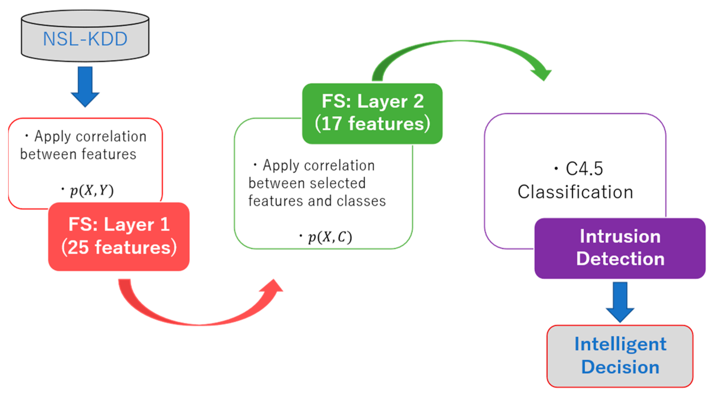
Eid et al. (2013) [57]	Pearson correlation	17	C4.5	NSL-KDD	ACC(%): 99.1, Time(s): 12.02
Wahba et al. (2015) [77]	CFS + IG (Adaboost)	13	NB	NSL-KDD	ACC(%): 99.3
Shahbaz et al. (2016) [68]	CFS	4	J48	NSL-KDD	ACC(%): 86.1, Time(s): <15
Ullah et al. (2017) [61]	IG	ISCX: 4 NSL-KDD: 6	J48	ISCX NSL-KDD	ACC(%): 99.70 (ISCX) 99.90 (NSL-KDD), Time(s): 15
Kushwaha et al. (2017) [63]	MI	5	Support vector machine (SVM)	KDDcup’99	ACC(%): 99.91
Moham madi et al. (2018) [66]	MI	/	least square version of SVM (LSSVM)	KDDcup’99, NSL-KDD, Kyoto 2006+	ACC(%): 94.31 (KDDcup’99) 98.31 (NSL-KDD) 99.11 (Kyoto 2006+)
Wang et al. (2019) [69]	Efficient CFS (MIFS + Symmetric Uncertainty)	KDDcup’99: 9 NSL-KDD: 10	One-class SVM	KDDcup’99, NSL-KDD	ACC(%): 99.85 (KDDcup’99) 98.64 (NSL-KDD), Time(s): 5.3 (KDDcup’99) 1.7 (NSL-KDD)

shows the comparison of filter-based feature selection techniques. The information contained in it is the FS method used, the number of features selected for a certain dataset, the detection method used, the dataset used, and the performance metrics of the techniques. The performance metrics of the techniques include the accuracy rate and the generation time of the detection model.

We provide Table 8 to give readers an idea of which studies used which filter-based techniques and how high the performance was that they could achieve in their respective experimental settings. The performance values mentioned in Table 8 are for reference only, and should not be used to judge the merits of the method. This is because the experimental settings and environments are different from each other. Readers who want to know some specific performance comparisons of different methods in the same experimental environment can read the corresponding papers in this table.

6. Summary

After introducing the importance of feature selection, this paper first provides an overview and classification of the existing feature selection techniques, and then the important and widely used category, filter-based methods, is described in detail, including general explanations, search algorithms, and relevance measures commonly used in such methods.

We organized the involved filter-based feature selection algorithms along their developmental trajectories, i.e., from basic correlation computation methods to the logic of complex algorithms that include both correlation computation and feature selection procedures. Due to the limitations of the Pearson correlation coefficient based on linear relationships and a chi-squared test based on statistics in measuring the correlation between variables, the most commonly-used metric in recent papers is information gain or mutual information based on information theory. The focus of this work is how to effectively screen features based on correlation and formulate corresponding rules. We believe this paper can serve as a useful guide for researchers and system developers, enabling readers not only to have a general overview of existing feature selection techniques but also to gain a more specific understanding of widely-used filter-based feature selection techniques.

In order for the reader to have a clear understanding of filter-based feature selection techniques, not only were many papers directly related to the topic required but also the necessary technical elements of this kind of technique (i.e., search algorithms and measures of relevance) were investigated in detail and placed in Together. In fact, in respective feature selection papers, these technical elements are usually not explained in detail, but only roughly mentioned. In addition, since readers need to grasp the status of this feature selection technique in the entire field of feature selection, a rough explanation of all feature selection techniques and the advantages of this technique were given first.

References

- Kaspersky Report. Available online: https://www.kaspersky.com/about/press-releases/2022_cybercriminals-attack-users-with-400000-new-malicious-files-daily---that-is-5-more-than-in-2021 (accessed on 26 January 2023).
- The Hacker News. Available online: https://thehackernews.com/2022/01/microsoft-mitigated-record-breaking-347.html (accessed on 28 January 2023).
- Hao, Z.; Feng, Y.; Koide, H.; Sakurai, K. A sequential detection method for intrusion detection system based on artificial neural networks. Int. J. Netw. Comput. 2020, 10, 213–226. [Google Scholar] [CrossRef]
- Cybercrime Magazine, Cybercrime to Cost the World $10.5 Trillion Annually by 2025. Available online: https://cybersecurityventures.com/cybercrime-damages-6-trillion-by-2021/ (accessed on 26 January 2023).
- Ravale, U.; Marathe, N.; Padiya, P. Feature selection based hybrid anomaly intrusion detection system using K means and RBF kernel function. Procedia Comput. Sci. 2015, 45, 428–435. [Google Scholar] [CrossRef] [Green Version]
- Chen, C.M.; Chen, Y.L.; Lin, H.C. An efficient network intrusion detection. Comput. Commun. 2010, 33, 477–484. [Google Scholar] [CrossRef]
- Shams, E.A.; Rizaner, A. A novel support vector machine based intrusion detection system for mobile ad hoc networks. Wirel. Netw. 2018, 24, 1821–1829. [Google Scholar] [CrossRef]
- Stein, G.; Chen, B.; Wu, A.S.; Hua, K.A. Decision tree classifier for network intrusion detection with GA-based feature selection. In Proceedings of the 43rd Annual Southeast Regional Conference, Kennesaw, GA, USA, 18–20 March 2005; Volume 2, pp. 136–141. [Google Scholar]
- Farnaaz, N.; Jabbar, M.A. Random forest modeling for network intrusion detection system. Procedia Comput. Sci. 2016, 89, 213–217. [Google Scholar] [CrossRef] [Green Version]
- Ashiku, L.; Dagli, C. Network intrusion detection system using deep learning. Procedia Comput. Sci. 2021, 185, 239–247. [Google Scholar] [CrossRef]
- Zl-Zubaidie, M.; Zhang, Z.; Zhang, J. RAMHU: A New Robust Lightweight Scheme for Mutual Users Authentication in Healthcare Applications. Secur. Commun. Netw. 2019, 2019, 1–26. [Google Scholar] [CrossRef]
- Saeys, Y.; Inza, I.; Larranaga, P. A review of feature selection techniques in bioinformatics. Bioinformatics 2007, 23, 2507–2517. [Google Scholar] [CrossRef] [Green Version]
- Bolón-Canedo, V.; Sánchez-Maroño, N.; Alonso-Betanzos, A. A review of feature selection methods on synthetic data. Knowl. Inf. Syst. 2013, 34, 483–519. [Google Scholar] [CrossRef]
- Soe, Y.N.; Feng, Y.; Santosa, P.I.; Hartanto, S.; Sakurai, K. Implementing lightweight IoT-IDS on raspberry pi using correlation-based feature selection and its performance evaluation. In Proceedings of the 33rd International Conference on Advanced Information Networking and Applications (AINA-2019), Matsue, Japan, 27–29 March 2019; pp. 458–469. [Google Scholar]
- Soe, Y.N.; Feng, Y.; Santosa, P.I.; Hartanto, S.; Sakurai, K. Towards a lightweight detection system for cyber attacks in the IoT environment using corresponding features. Electronics 2020, 9, 144. [Google Scholar] [CrossRef] [Green Version]
- Image Filtering Overview. Available online: https://www.ni.com/ja-jp/innovations/white-papers/06/image-filtering-overview.html (accessed on 5 March 2023).
- Zhang, X.; He, S.; Stojanovic, V.; Luan, X.; Liu, F. Finite-time asynchronous dissipative filtering of conic-type nonlinear Markov jump systems. Sci. China Inf. Sci. 2021, 64, 152206. [Google Scholar] [CrossRef]
- Cheng, P.; Wang, J.; He, S.; Luan, X.; Liu, F. Observer-based asynchronous fault detection for conic-type nonlinear jumping systems and its application to separately excited DC motor. IEEE Trans. Circuits Syst. I Regul. Pap. 2020, 67, 951–962. [Google Scholar] [CrossRef]
- Cheng, P.; He, S.; Stojanovic, V.; Luan, X.; Liu, F. Fuzzy fault detection for Markov jump systems with partly accessible hidden information: An event-triggered approach. IEEE Trans. Cybern. 2022, 52, 7352–7361. [Google Scholar] [CrossRef] [PubMed]
- Sharma, N.; Arora, B. A Critical Review of Feature Selection Techniques for Network Anomaly Detection: Methodologies, Challenges, Evaluation, and Opportunities. 2022. Available online: https://www.researchsquare.com/article/rs-1940841/v1 (accessed on 26 January 2023).
- Yu, L.; Liu, H. Feature selection for high-dimensional data: A fast correlation-based filter solution. In Proceedings of the 20th International Conference on Machine Learning (ICML-2003), Washington, DC, USA, 21–24 August 2003; pp. 856–863. [Google Scholar]
- Senliol, B.; Gulgezen, G.; Yu, L.; Cataltepe, Z. Fast correlation based filter (FCBF) with a different search strategy. In Proceedings of the 23rd International Symposium on Computer and Information Sciences 2008, Istanbul, Turkey, 27–29 October 2008; pp. 1–4. [Google Scholar] [CrossRef]
- Wah, Y.B.; Ibrahim, N.; Hamid, H.A.; Abdul-Rahman, S.; Fong, S. Feature selection methods: Case of filter and wrapper approaches for maximising classification accuracy. Pertanika J. Sci. Technol. 2018, 26, 329–340. [Google Scholar]
- Hoque, N.; Bhattacharyya, D.K.; Kalita, J.K. MIFS-ND: A mutual information-based feature selection method. Expert Syst. Appl. 2014, 41, 6371–6385. [Google Scholar] [CrossRef]
- Ladha, L.; Deepa, T. Feature selection methods and algorithms. Int. J. Comput. Sci. Eng. IJCSE 2011, 3, 1787–1797. [Google Scholar]
- Cantu-Paz, E. Feature subset selection, class separability, and genetic algorithms. In Proceedings of the Genetic and Evolutionary Computation—GECCO 2004: Genetic and Evolutionary Computation Conference, Seattle, WA, USA, 26–30 June 2004; Springer: Berlin/Heidelberg, Germany, 2004; pp. 959–970. [Google Scholar]
- Bolón-Canedo, V.; Sánchez-Marono, N.; Alonso-Betanzos, A.; Benítez, J.M.; Herrera, F. A review of microarray datasets and applied feature selection methods. Inf. Sci. 2014, 282, 111–135. [Google Scholar] [CrossRef]
- Thakkar, A.; Lohiya, R. A survey on intrusion detection system: Feature selection, model, performance measures, application perspective, challenges, and future research directions. Artif. Intell. Rev. 2022, 55, 453–563. [Google Scholar] [CrossRef]
- Sánchez-Maroño, N.; Alonso-Betanzos, A.; Calvo-Estévez, R.M. A wrapper method for feature selection in multiple classes datasets. In Proceedings of the International Work-Conference on Artificial Neural Networks 2009, Limassol, Cyprus, 14–17 September 2009; Springer: Berlin/Heidelberg, Germany, 2009; pp. 456–463. [Google Scholar]
- Piao, Y.; Piao, M.; Park, K.; Ryu, K.H. An ensemble correlation-based gene selection algorithm for cancer classification with gene expression data. Bioinformatics 2012, 28, 3306–3315. [Google Scholar] [CrossRef] [Green Version]
- Yusta, S.C. Different metaheuristic strategies to solve the feature selection problem. Pattern Recognit. Lett. 2009, 30, 525–534. [Google Scholar] [CrossRef]
- Jović, A.; Brkić, K.; Bogunović, N. A review of feature selection methods with applications. In Proceedings of the 38th International Convention on Information and Communication Technology, Electronics and Microelectronics (MIPRO), Opatija, Croatia, 25–29 May 2015; pp. 1200–1205. [Google Scholar] [CrossRef]
- Zuech, R.; Khoshgoftaar, T.M. A survey on feature selection for intrusion detection. In Proceedings of the 21st ISSAT International Conference on Reliability and Quality in Design, Philadelphia, PA, USA, 6–8 August 2015; pp. 150–155. [Google Scholar]
- Guyon, I.; Weston, J.; Barnhill, S.; Vapnik, V. Gene selection for cancer classification using support vector machines. Mach. Learn. 2002, 46, 389–422. [Google Scholar] [CrossRef]
- Maldonado, S.; Weber, R.; Basak, J. Simultaneous feature selection and classification using kernel-penalized support vector machines. Inf. Sci. 2011, 181, 115–128. [Google Scholar] [CrossRef]
- Loh, W.Y. Classification and regression trees. Wiley Data Min. Knowl. Discov. 2011, 1, 14–23. [Google Scholar] [CrossRef]
- Patel, H.H.; Prajapati, P. Study and analysis of decision tree based classification algorithms. Int. J. Comput. Sci. Eng. 2018, 6, 74–78. [Google Scholar] [CrossRef]
- Sandri, M.; Zuccolotto, P. Variable selection using random forests. In Data Analysis, Classification and the Forward Search, Proceedings of the Meeting of the Classification and Data Analysis Group (CLADAG) of the Italian Statistical Society, University of Parma, Parma, Italy, 6–8 June 2005; Springer: Berlin/Heidelberg, Germany, 2005; pp. 263–270. [Google Scholar]
- Cawley, G.; Talbot, N.; Girolami, M. Sparse multinomial logistic regression via bayesian l1 regularisation. In Proceedings of the Advances in Neural Information Processing Systems 19 (NIPS 2006), Vancouver, BC, Canada, 4–5 December 2006; Volume 19. [Google Scholar]
- Das, S. Filters, wrappers and a boosting-based hybrid for feature selection. InIcml 2001, 1, 74–81. [Google Scholar]
- Hsu, H.H.; Hsieh, C.W.; Lu, M.D. Hybrid feature selection by combining filters and wrappers. Expert Syst. Appl. 2011, 38, 8144–8150. [Google Scholar] [CrossRef]
- Naqvi, S. A Hybrid Filter-Wrapper Approach for Feature Selection. Master’s Thesis, the Department of Technology, Örebro University, Örebro, Sweden, 2012. Available online: http://www.diva-portal.org/smash/get/diva2:567115/FULLTEXT01.pdf (accessed on 5 March 2023).
- Cadenas, J.M.; Garrido, M.C.; MartíNez, R. Feature subset selection filter–wrapper based on low quality data. Expert Syst. Appl. 2013, 40, 6241–6252. [Google Scholar] [CrossRef]
- Oh, I.S.; Lee, J.S.; Moon, B.R. Hybrid genetic algorithms for feature selection. IEEE Trans. Pattern Anal. Mach. Intell. 2004, 26, 1424–1437. [Google Scholar]
- Ali, S.I.; Shahzad, W. A feature subset selection method based on conditional mutual information and ant colony optimization. Int. J. Comput. Appl. 2012, 60, 5–10. [Google Scholar]
- Sarafrazi, S.; Nezamabadi-Pour, H. Facing the classification of binary problems with a GSA-SVM hybrid system. Math. Comput. Model. 2013, 57, 270–278. [Google Scholar] [CrossRef]
- Ma, S.; Huang, J. Penalized feature selection and classification in bioinformatics. Brief. Bioinform. 2008, 9, 392–403. [Google Scholar] [CrossRef] [PubMed] [Green Version]
- Zou, H.; Hastie, T. Regularization and variable selection via the elastic net. J. R. Stat. Soc. Ser. B Stat. Methodol. 2005, 67, 301–320. [Google Scholar] [CrossRef] [Green Version]
- Nakashima, M.; Sim, A.; Kim, Y.; Kim, J.; Kim, J. Automated feature selection for anomaly detection in network traffic data. ACM Trans. Manag. Inf. Syst. 2021, 12, 1–28. [Google Scholar] [CrossRef]
- Liu, H.; Motoda, H. Feature Selection for Knowledge Discovery and Data Mining; Springer Science & Business Media: Berlin/Heidelberg, Germany, 2012; Volume 454. [Google Scholar]
- Kittler, J. Feature set search algorithms. In Pattern Recognition and Signal Processing; Springer: Dordrecht, The Netherlands, 1978. [Google Scholar]
- Miller, A. Subset Selection in Regression; Monographs on Statistics and Applied Probability 95; Chapman & Hall/CRC: Boca Raton, FL, USA, 2002. [Google Scholar]
- Hall, M.A. Correlation-Based Feature Selection for Machine Learning. Ph.D. Thesis, The University of Waikato, Hamilton, New Zealand, 1999. [Google Scholar]
- Winston, P.H. Artificial Intelligence; Addison-Wesley Longman Publishing Co., Inc.: Boston, MA, USA, 1984. [Google Scholar]
- Holland, J.H. Adaptation in Natural and Artificial Systems; An Introductory Analysis with Applications to Biology, Control, and Artificial Intelligence; MIT Press: Cambridge, MA, USA; London, UK, 1992. [Google Scholar]
- Teukolsky, S.A.; Flannery, B.P.; Press, W.H.; Vetterling, W.T. Numerical Recipes in C; SMR.693; WH Press: Cambridge, MA, USA, 1992.
- Eid, H.F.; Hassanien, A.E.; Kim, T.H.; Banerjee, S. Linear correlation-based feature selection for network intrusion detection model. In Proceedings of the International Conference on Security of Information and Communication Networks 2013, Cairo, Egypt, 3–5 September 2013; Springer: Berlin/Heidelberg, Germany, 2013; pp. 240–248. [Google Scholar]
- Li, Y.; Fang, B.X.; Chen, Y.; Guo, L. A lightweight intrusion detection model based on feature selection and maximum entropy model. In Proceedings of the 2006 International Conference on Communication Technology, Guilin, China, 27–30 November 2006; pp. 1–4. [Google Scholar]
- Liu, H.; Setiono, R. Chi2: Feature selection and discretization of numeric attributes. In Proceedings of the 7th IEEE International Conference on Tools with Artificial Intelligence, Herndon, VA, USA, 5–8 November 1995; pp. 388–391. [Google Scholar]
- Salzberg, S.L. C4.5: Programs for Machine Learning by J. Ross Quinlan. Morgan Kaufmann Publishers, Inc., 1993. Mach. Learn. 1994, 16, 235–240. [Google Scholar] [CrossRef] [Green Version]
- Ullah, I.; Mahmoud, Q.H. A filter-based feature selection model for anomaly-based intrusion detection systems. In Proceedings of the 2017 IEEE International Conference on Big Data (Big Data) 2017, Boston, MA, USA, 11–14 December 2017; pp. 2151–2159. [Google Scholar]
- Cover, T.M.; Thomas, J.A. Elements of Information Theory; Wiley: Hoboken, NJ, USA, 2012. [Google Scholar]
- Kushwaha, P.; Buckchash, H.; Raman, B. Anomaly based intrusion detection using filter based feature selection on KDD-CUP 99. In Proceedings of the TENCON 2017—2017 IEEE Region 10 Conference, Penang, Malaysia, 5–8 November 2017; pp. 839–844. [Google Scholar]
- Kraskov, A.; Stögbauer, H.; Grassberger, P. Estimating mutual information. Phys. Rev. E 2004, 69, 066138. [Google Scholar] [CrossRef] [Green Version]
- Peng, H.; Long, F.; Ding, C. Feature selection based on mutual information criteria of max-dependency, max-relevance, and min-redundancy. IEEE Trans. Pattern Anal. Mach. Intell. 2005, 27, 1226–1238. [Google Scholar] [CrossRef] [PubMed]
- Mohammadi, S.; Desai, V.; Karimipour, H. Multivariate mutual information-based feature selection for cyber intrusion detection. In Proceedings of the 2018 IEEE Electrical Power and Energy Conference (EPEC), Toronto, ON, Canada, 10–11 October 2018; pp. 1–6. [Google Scholar]
- Battiti, R. Using mutual information for selecting features in supervised neural net learning. IEEE Trans. Neural Netw. 1994, 5, 537–550. [Google Scholar] [CrossRef] [Green Version]
- Shahbaz, M.B.; Wang, X.; Behnad, A.; Samarabandu, J. On efficiency enhancement of the correlation-based feature selection for intrusion detection systems. In Proceedings of the 2016 IEEE 7th Annual Information Technology, Electronics and Mobile Communication Conference (IEMCON), Vancouver, BC, Canada, 13–15 October 2016; pp. 1–7. [Google Scholar]
- Wang, W.; Du, X.; Wang, N. Building a cloud IDS using an efficient feature selection method and SVM. IEEE Access 2018, 7, 1345–1354. [Google Scholar] [CrossRef]
- Tavallaee, M.; Bagheri, E.; Lu, W.; Ghorbani, A.A. A detailed analysis of the KDD CUP 99 data set. In Proceedings of the 2009 IEEE Symposium on Computational Intelligence for Security and Defense Applications, Ottawa, ON, Canada, 8–10 July 2009; pp. 1–6. [Google Scholar]
- Revathi, S.; Malathi, A. A detailed analysis on NSL-KDD dataset using various machine learning techniques for intrusion detection. Int. J. Eng. Res. Technol. IJERT 2013, 2, 1848–1853. [Google Scholar]
- Lashkari, A.H.; Draper-Gil, G.; Mamun, M.S.I.; Ghorbani, A.A. Characterization of Tor Traffic Using Time Based Features. In Proceedings of the International Conference on Information Systems Security and Privacy, Porto, Portugal, 19–21 February 2017; pp. 253–262. [Google Scholar]
- D’hooge, L.; Wauters, T.; Volckaert, B.; De Turck, F. Inter-dataset generalization strength of supervised machine learning methods for intrusion detection. J. Inf. Secur. Appl. 2020, 54, 102564. [Google Scholar] [CrossRef]
- Hindy, H.; Bayne, E.; Bures, M.; Atkinson, R.; Tachtatzis, C.; Bellekens, X. Machine learning based IoT intrusion detection system: An MQTT case study (MQTT-IoT-IDS2020 dataset). In Selected Papers from the 12th International Networking Conference; Springer International Publishing: Cham, Switzerland, 2020; pp. 73–84. [Google Scholar]
- Ullah, I.; Mahmoud, Q.H. Design and development of a deep learning-based model for anomaly detection in IoT networks. IEEE Access 2021, 9, 103906–103926. [Google Scholar] [CrossRef]
- Nguyen, H.; Franke, K.; Petrovic, S. Improving effectiveness of intrusion detection by correlation feature selection. In Proceedings of the 2010 International Conference on Availability, Reliability and Security 2010, Krakow, Poland, 15–18 February 2010; pp. 17–24. [Google Scholar]
- Wahba, Y.; ElSalamouny, E. ElTaweel, GImproving the performance of multi-class intrusion detection systems using feature reduction. arXiv 2015, arXiv:1507.06692. [Google Scholar]