Improved VIV Response Prediction Using Adaptive Parameters and Data Clustering

Abstract

Slender marine structures such as deep-water riser systems are continuously exposed to currents, leading to vortex-induced vibrations (VIV) of the structure. This may result in amplified drag loads and fast accumulation of fatigue damage. Consequently, accurate prediction of VIV responses is of great importance for the safe design and operation of marine risers. Model tests with elastic pipes have shown that VIV responses are influenced by many structural and hydrodynamic parameters, which have not been fully modelled in present frequency domain VIV prediction tools. Traditionally, predictions have been computed using a single set of hydrodynamic parameters, often leading to inconsistent prediction accuracy when compared with observed field measurements and experimental data. Hence, it is necessary to implement a high safety factor of 10–20 in the riser design, which increases development costs and adds extra constraints in the field operation. One way to compensate for the simplifications in the mathematical prediction model is to apply adaptive parameters to describe different riser responses. The objective of this work is to demonstrate a new method to improve the prediction consistency and accuracy by applying adaptive hydrodynamic parameters. In the present work, a four-step approach has been proposed: First, the measured VIV response will be analysed to identify key parameters to represent the response characteristics. These parameters will be grouped by using data clustering algorithms. Secondly, optimal hydrodynamic parameters will be identified for each data group by optimisation against measured data. Thirdly, the VIV response using the obtained parameters will be calculated and the prediction accuracy evaluated. Last but not least, classification algorithms will be applied to determine the correct hydrodynamic parameters to be used for new cases. An iteration of the previous steps may be needed if the prediction accuracy of the new case is not satisfactory. This concept has been demonstrated with examples from experimental data.

1. Introduction

Risers and pipelines are important structural elements in offshore oil and gas exploration and development. Vortex-induced vibrations (VIVs) cause cyclic loads and an amplified drag force on the cylindrical structures. Consequently, severe fatigue damage may be accumulated and mechanical failure can occur. Therefore, in the design and operation of marine risers, it is important to understand the global VIV responses of deep-water risers and marine pipelines and get accurate predictions of the responses.

Semi-empirical VIV prediction tools such as VIVANA [1], Shear7 [2], and VIVA [3] are tools commonly used by the industry. These prediction tools consist of a structural model and a hydrodynamic load model. The structural model may be based on normal or complex mode superposition or use finite elements with coupled equations. The hydrodynamic load model is based on the “strip theory”. The hydrodynamic force and frequency depends on local flow conditions, response amplitude, and structural geometry. The load model and the empirical parameters are developed from model tests using rigid cylinders and flexible pipes.

The hydrodynamic parameters required by the prediction tools are normally generalised from rigid cylinder forced motion tests. In such tests, a rigid cylinder is towed through the water at a constant speed (U) and forced to oscillate under designed motion amplitudes (A) and frequencies ($f_{osc}$), which approximate the actual trajectories of the cross-section of a flexible pipe. The hydrodynamic coefficients are derived from the force measurement of the rigid cylinder section [4,5]. Despite the efforts to obtain hydrodynamic data from realistic cylinder motions [6,7,8,9], the hydrodynamic parameters used in the present prediction tools are still based on tests with one-dimensional cross-flow (CF) harmonic motions, neglecting in-line vibrations that are also present. Often these tests are carried out in conditions characterised by sub-critical Reynolds numbers, while the riser in the field will experience flow conditions in the critical or super-critical flow regimes.

The effects of variations in the Reynolds number were studied on a full scale pipe section by [10,11,12]. It was found that the hydrodynamic coefficient is sensitive to the Reynolds number. In addition, the surface roughness ratio was also found to be an important parameter. These effects have not been accounted for in the present VIV prediction tools.

VIV tests with elastic pipe/riser models have mainly focused on global responses [13,14,15,16,17,18,19] where bending strain, curvature, and/or acceleration are typically measured at discrete locations along the test model under uniform and shear current conditions. The measured cross-section motion trajectories found from such tests are far from harmonic [8]. The hydrodynamic force coefficients along the test model can be estimated by an inverse analysis method [20,21]. This method basically uses measured response data to calculate the external VIV loads by assuming that the mechanical properties (stiffness, mass, etc.) are known. The hydrodynamic coefficients estimated by inverse analysis also show deviation from results of rigid cylinder tests. In such tests, small-scale models are normally used, which means that the Reynolds number is relatively low.

Inconsistent prediction accuracy is seen when benchmarked against elastic cylinder tests in ideal laboratory conditions, where tests are carried out under constant and unidirectional flow with densely spaced and accurate measurements [22]. Even larger discrepancies have been seen when compared to full-scale field measurement data [23]. Part of the reasons for these discrepancies are oversimplifications in the hydrodynamic load model and the associated parameters applied in the prediction tools.

The objective of this work is to introduce a new method to improve the prediction consistency and accuracy by applying adaptive hydrodynamic parameters. In the present study, the complexity of VIV responses is first explained with typical model test examples in Section 2. The limitations of the present VIV prediction tools with built-in empirical parameters is discussed in Section 3. This provides the background and reasons for using adaptive parameters to compensate for the simplifications in the numerical models. The concept of adaptive parameters is then discussed in Section 4, with examples to demonstrate the possible improvement in VIV predictions. Machine learning (ML) has been applied, where data clustering algorithms have been used to group the response data from various model tests and where each group is associated with a set of parameters. Classification algorithms have been used to select the optimum parameters for the new data. Potential applications to improve riser design practice and field monitoring are discussed in Section 4.

2. Characteristics of VIV Responses

It is known that the current profile can have a significant influence on VIV responses of deep-water riser systems. There is a lack of prediction models for describing VIV responses subjected to three-dimensional (3D) current [24]. Therefore, in the present design practice, a unidirectional (2D) current profile is assumed. Sheared or uniform 2D currents are normally simulated in model tests. If the current profile is linearly sheared, the excitation region is well defined in the high current speed area. If the shear profile is similar to the Gulf of Mexico profile [25], the excitation region is distributed over several locations along the pipe length. Since the sheared current profile is more realistic for deep-water riser systems, five different VIV model tests with sheared current profiles were selected to be further investigated in the present work, with a focus on the CF response.

2.1. Influence of Travelling Speed and Bending Stiffness on VIV Responses

The responses of a elastic pipe can be influenced by the longitudinal travelling speed of the VIV response [26].

The theoretical travel speed of oscillations of an infinitely long tensioned string and an untensioned beam are calculated by the following equations:

Tensioned string:

$$C_s=\sqrt{\frac{T}{m}}.$$

(1)

Un-tensioned beam:

$$C_{b,CF/IL}=\sqrt[4]{\frac{{\omega }_{CF/IL}^2,EI}{m}}$$

(2)

where, m is the mass per unit length; $EI$ is the bending stiffness; T is the tension and $\omega$ is the response frequency in IL and CF directions.

For a tension-dominated string, the travel speed will be independent of the response frequency. This means that the wave speeds of responses in IL and CF directions are the same. For a beam with controlled bending stiffness, the longitudinal travelling speed depends on the response frequency. This means the CF response at the primary frequency $\omega$ will be travelling along the pipe with a different speed than the IL response. Thus, the motion trajectories will constantly vary along the pipe. This will affect the CF VIV response both at the primary frequency $\omega$ and the third-order frequency component $3\times \omega$, together with other factors [26].

One way to quantify the importance of the bending stiffness is to evaluate the natural frequencies of the pipe model. Elastic pipe models in VIV tests could be simplified as tensioned elastic beams. Both tension and bending stiffness contribute to the total stiffness. The natural frequencies of a tensioned beam are given by the following equations:

For a tensioned string:

$$f_{n,s}=\frac{n}{2L}\sqrt{\frac{T}{m}}.$$

(3)

For an untensioned beam:

$$f_{n,b}=\frac{n^2\pi }{2L^2}\sqrt{\frac{EI}{m}}.$$

(4)

For a tensioned beam:

$$f_{n,tot}=\sqrt{f_{n,s}^2+f_{n,b}^2},$$

(5)

where L is the pipe length and n is the mode number.

The relative magnitude of the bending stiffness can be quantified by the frequency ratio

$$F=f_{n,b}/f_{n,tot}.$$

(6)

The higher the value of this parameter, the stronger the influence of the bending stiffness will be. Furthermore, the travelling speed will be increasingly different in the IL and CF directions.

2.2. Selected Elastic Pipe Model Tests

Performing experiments on a scaled elastic riser or on pipeline models is a common approach to study the global response. The measurements are used to validate various numerical VIV prediction tools. In this section, several representative model tests of elastic bare riser models are reviewed, and the physical properties are summarised in

Table 1. Summary of physical properties of the riser/pipe model of various elastic model vortex-induced vibration (VIV) tests.

Test	Length $\mathit{L}\left(\mathit{m}\right)$	Diameter $\mathit{D}\left(\mathit{m}\right)$	Mass Ratio ${\mathit{m}}^{*}$	Bending Stiffness $\mathit{EI}\left({\mathit{Nm}}^{\mathbf{2}}\right)$	Mean Tension $\overline{\mathit{T}}\left(\mathit{N}\right)$
NDP high-mode test	38	0.027	1.632	37.2	4000
Shell high-mode test (pipe 2)	38	0.030	1.54	572.3	4000
Hanøytangen	90	0.030	3.13	3639	3700
ExxonMobil rotating rig test	9.63	0.02	2.17	135.4	700
Miami II test	152.4	0.0363	1.268	613	3225

. A description of the test setup can be found in Appendix A.

2.3. Characteristics of VIV Responses of an Elastic Pipe in Sheared Current

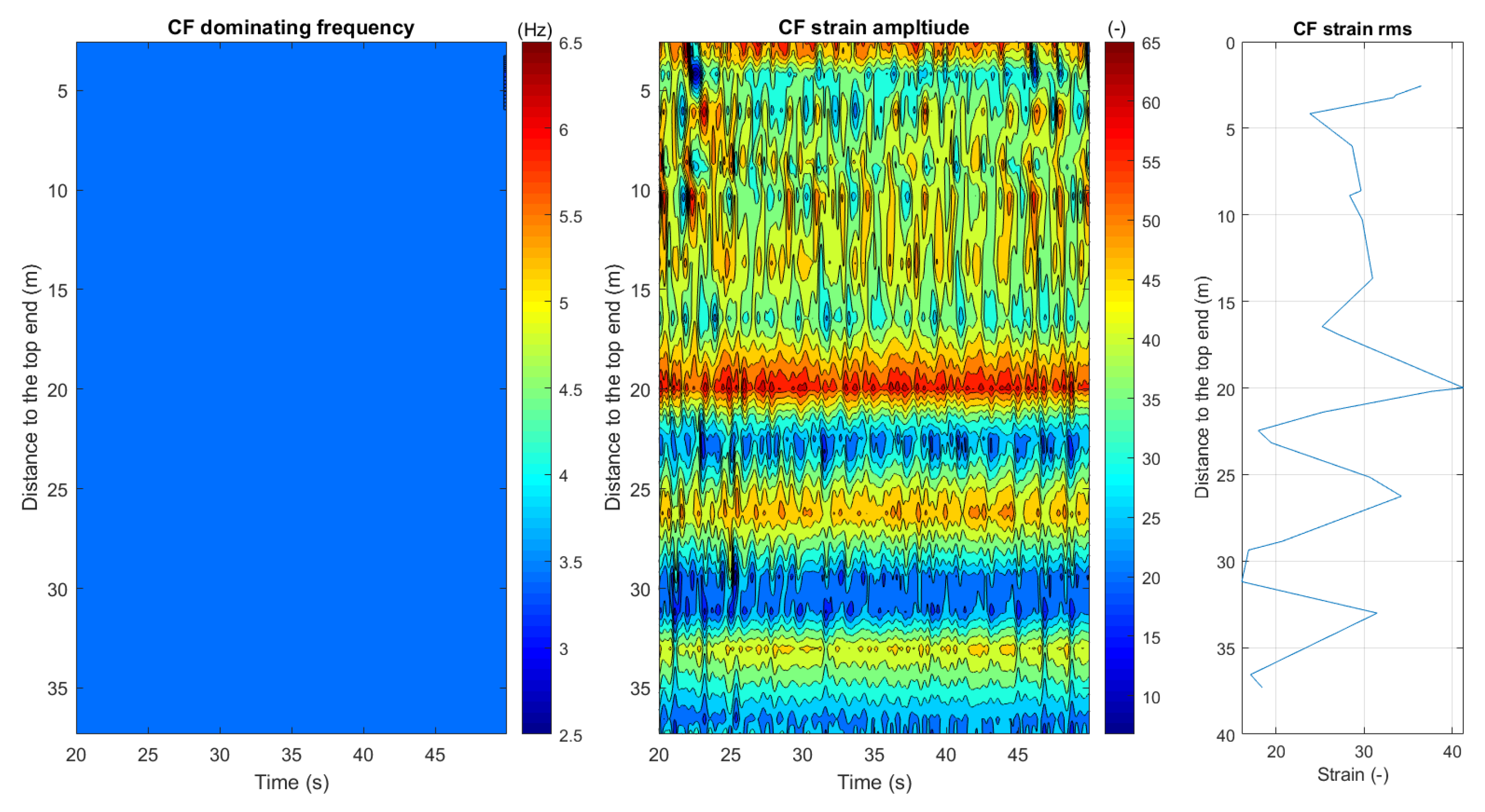
The shedding frequency is given by $f_s=StU/D$, where St is the Strouhal number, U is the flow speed, and D is the pipe diameter. In a sheared flow, the shedding frequency may vary along the length of the pipe. In addition, the response frequency and mode are known to vary in time even under a constant flow speed due to the flow instability. The variation of the dominating response frequency in space and time can be extracted from wavelet analysis of the measured response signals along the length of the test pipe [27]. 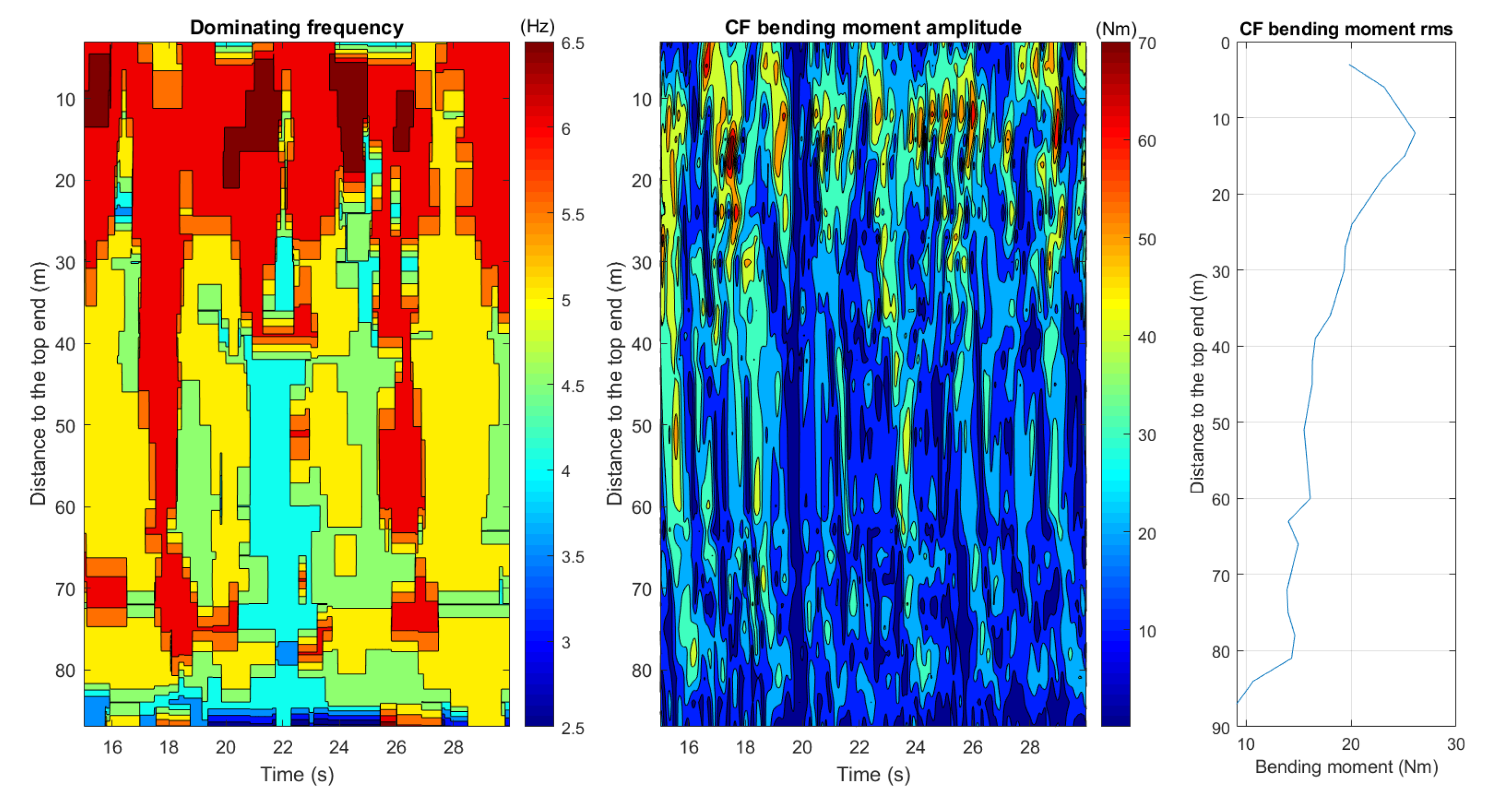The frequency composition can be different for a tension-dominated pipe vibrating at a low mode (∼5), as shown in Figure 1, or a bending-stiffness-dominated pipe responding at a high mode (∼25), as shown in Figure 2. The response is dominated by a single frequency (≈3.5 Hz) for the former, even when subjected to a sheared current. However, the frequency variation is much more complicated for high-mode VIV responses, as shown in Figure 2. Higher frequencies are observed at the high flow speed region at the top of the riser, and lower frequencies close to the bottom where the flow speed decreases to zero (“space sharing” [1]), e.g., 15–17 s. “Time sharing” [28] of the frequency is also observed. The experimental results show that the response frequency varies along the length of the pipe. If well synchronised, fewer frequencies tend to dominate longer sections of the pipe. The response will also be stable with higher motion amplitudes. On the other hand, the response will be controlled by the local shedding process when the synchronisation breaks down, which leads to more frequencies and chaotic responses with lower motion amplitudes.

Such behaviour is related to the bending stiffness of the structure, which can affect the response-wave propagation speed and motion orbits. It is also related to the presence of the travelling waves. The higher the mode, the more a travelling wave response will be present, as discussed earlier. In addition, large tension variation has been observed in some of the high-mode VIV response tests, which may also contribute to the instability of the response.

The model tests with long elastic cylinder models cover a large variation of riser dimensions, cross-sectional properties, boundary conditions, and flow conditions. This calls for an improved understanding the VIV behaviours of different riser configurations and numerical tools with increased robustness and specialised treatment of the response characteristics [29].

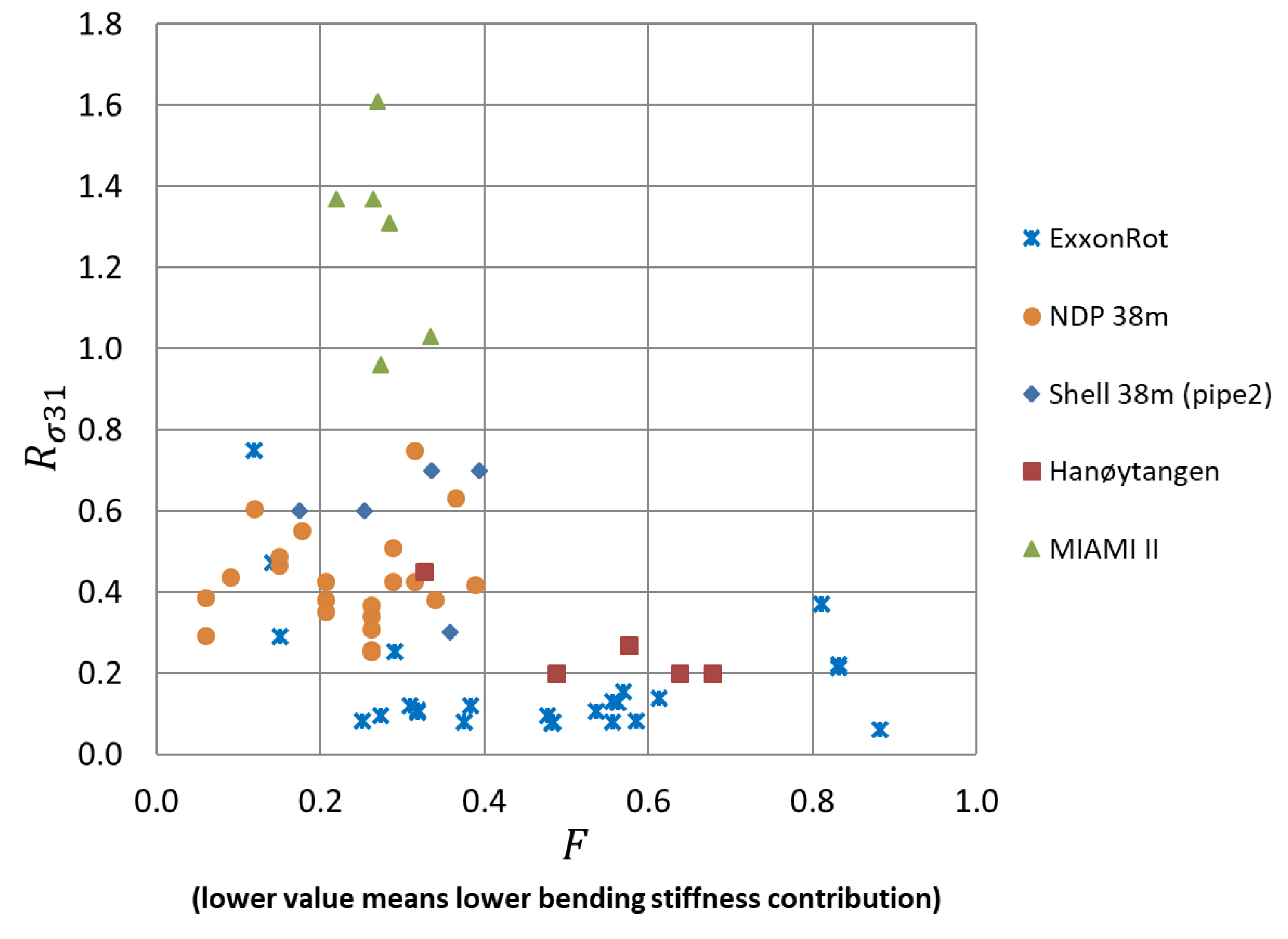
The characteristics of VIV responses subjected to a sheared current profile have been studied in [26], as summarised in

Table 2. Summary of response characteristics from selected model tests [29].

TEST	Mode Order	Travelling/Standing Wave Response	Stiffness	3rd Order Harmonic Stress
NDP high-mode test	4–14	Increased travelling wave	Tension-dominated	Medium
		response with mode order
Shell high-mode test (pipe 2)	2–14	Increased travelling wave	Tension-dominated	Medium
		response with mode order
Hanøytangen test	10–27	Travelling waves	Bending-dominated	Low
Miami II test	25–39	Travelling waves	Tension-dominated	High
ExxonMobil rotating rig test	1–7	Standing waves	Bending-dominated	Low

and in Figure 3. In this figure, the stress ratio ($R_{\sigma 31}$) is defined as the ratio between the standard deviation of the maximum stress measured at ($3\times \omega$) and ($1\times \omega$) frequencies along the length of the test pipe.

$$R_{\sigma 31}=\frac{max\left(std\left({\sigma }_3\right)\right)}{max\left(std\left({\sigma }_1\right)\right)}$$

(7)

The bending stiffness ratio ($F=f_{n,b}/f_{n,tot}$) indicates how significant the bending stiffness contribution is to the total stiffness of the structure. The main observation from Figure 3 is that the stress ratio increases when the bending stiffness is of less importance. In addition, the stress ratio can be very different depending on the presence of travelling waves in the response, which is indicated by the data points around $f_{n,b}/f_{n,tot}=0.3$. This study shows that there needs to be long regions of stable and favourable motion orbits inside the excitation region in order to get significant third-order ($3\times \omega$) harmonic stresses. This seems to require the following conditions:

• Response dominated by travelling waves;
• Low relative bending stiffness contribution;
• Stationary response.

These conditions will not only influence the higher harmonic stress but also the responses at the primary shedding frequency ($1\times \omega$). The strong response at the primary shedding frequency is normally associated with a strong higher harmonic response [26].

3. Limitations of the Present Empirical VIV Prediction Tools

Present empirical VIV prediction tools are based on a response frequency model and a load model with a hydrodynamic coefficient database. The structural model is linear.

3.1. Response Frequency Model

In order to be able to describe the frequency variations in space and time, the prediction tools include “space sharing” and/or “time sharing” models. In the space-sharing model, the responses in different sections of the pipe may be dominated by different frequencies, but these frequencies will be constant in time. In contrast, time sharing is assumed to appear as a sequence of single-frequency responses [1]. These frequency models are reasonable approximations of the observed physical process, but with strong simplifications. There is also a lack of criteria when to switch between space sharing and time sharing models in the analysis, and consequently, the analysis will be either time sharing or space sharing when it should have been a combination of the two.

3.2. Hydrodynamic Parameters

Present empirical VIV prediction tools rely on hydrodynamic parameters generalised from rigid cylinder tests. The CF hydrodynamic data is based on tests with pure CF harmonic motions [4]. The excitation coefficients are dependent on the motion amplitude ratio $\left(A/D\right)$ and the non-dimensional frequency $(f_{osc}D/U)$. However, it is known that hydrodynamic coefficients of an elastic pipe will be strongly influenced by IL motions, which are not present the in one-dimensional motion tests [5,25,30].

Inverse analysis has also been applied to estimate CF hydrodynamic coefficients of an elastic pipe from measured response data directly [20]. The results show that the excitation coefficients of an elastic cylinder are different compared to those from a rigid cylinder with pure CF motions. It is also demonstrated that the coefficients are further influenced by multiple frequency variations in space and time. These frequencies compete for energy, which leads to less stable vortex shedding and more chaotic responses. Hence, the magnitudes of the excitation coefficients are smaller compared to that of a stable response dominated by one single frequency. These effects have not been fully accounted for in the existing hydrodynamic coefficients.

The hydrodynamic coefficient database can be modelled by a set of parameters. An optimisation technique has been applied to obtain best-fit hydrodynamic parameters by calibrating the model prediction against measured response data from elastic cylinder tests. The space-sharing model has been used in the calibration. The fatigue prediction using calibrated parameters agrees well with the measurements [22,31].

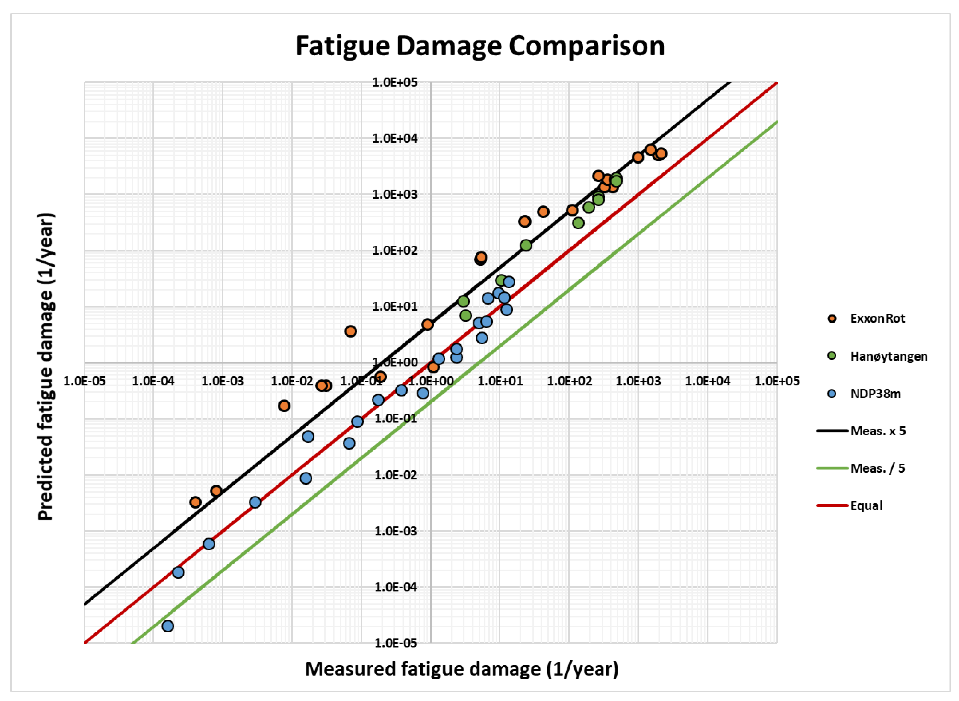
However, increased discrepancy between prediction and measurement has been observed when the same set of hydrodynamic parameters is applied to predict VIV responses of different model tests, as illustrated in Figure 4. The ratio between the measured maximum fatigue damage and the predicted results exceeds a factor of 5 for about 26% of the 57 cases. Prediction errors within a factor of 3 are found in 53% of the cases. The largest deviation shows over-predictions by a factor of 52. In the present study, one single slope S–N curve has been applied to all of the cases in the fatigue calculation, which is presented in

$$\log \left(\mathrm{N}\right)=\log \left(\mathrm{a}\right)-\mathrm{mlog}\left(\mathrm{S}\right),$$

(8)

where N is the predicted number of cycles to failure under stress range S (in Mpa). m is the inverse slope of the S–N curve, and log used in the notation is log to the base 10. The S–N curve constants m and a are 3 and 11.63, respectively.

4. Improved VIV Prediction Accuracy With Adaptive Hydrodynamic Parameters

4.1. Concept

The challenge is how to compensate for the simplicity in the load model and the hydrodynamic parameters so that the prediction matches the actual VIV responses from measured data. Optimisation is one way to obtain best-fit parameters; however, it is difficult to obtain a single set of parameters that gives accurate predictions for all cases, as shown in Figure 4. The more complicated cases included, the less robust the obtained parameters will be. The proposed strategy is therefore to apply adaptive parameters that reflect the different response patterns. A four-step approach is applied in the present study:

• First, the measured VIV response will be analysed to identify key parameters to represent the response characteristics. These parameters will be grouped by similarity using data clustering algorithms.
• Secondly, optimal hydrodynamic parameters will be identified for each data cluster by optimisation against measured data within that cluster.
• Thirdly, the VIV response using the obtained parameters will be calculated and the prediction accuracy evaluated.
• Last but not the least, new cases must be assigned to a cluster in order to determine the correct hydrodynamic parameters. An iteration of the previous steps may be needed if the prediction accuracy of the new case is not satisfactory.

In the present study, CF VIV responses at the primary response frequency have been evaluated. The main objective of the present work is to demonstrate the validity/applicability of the concept and hence, simplifications in the analysis procedure have been made.

4.2. Clustering the Model Test Data

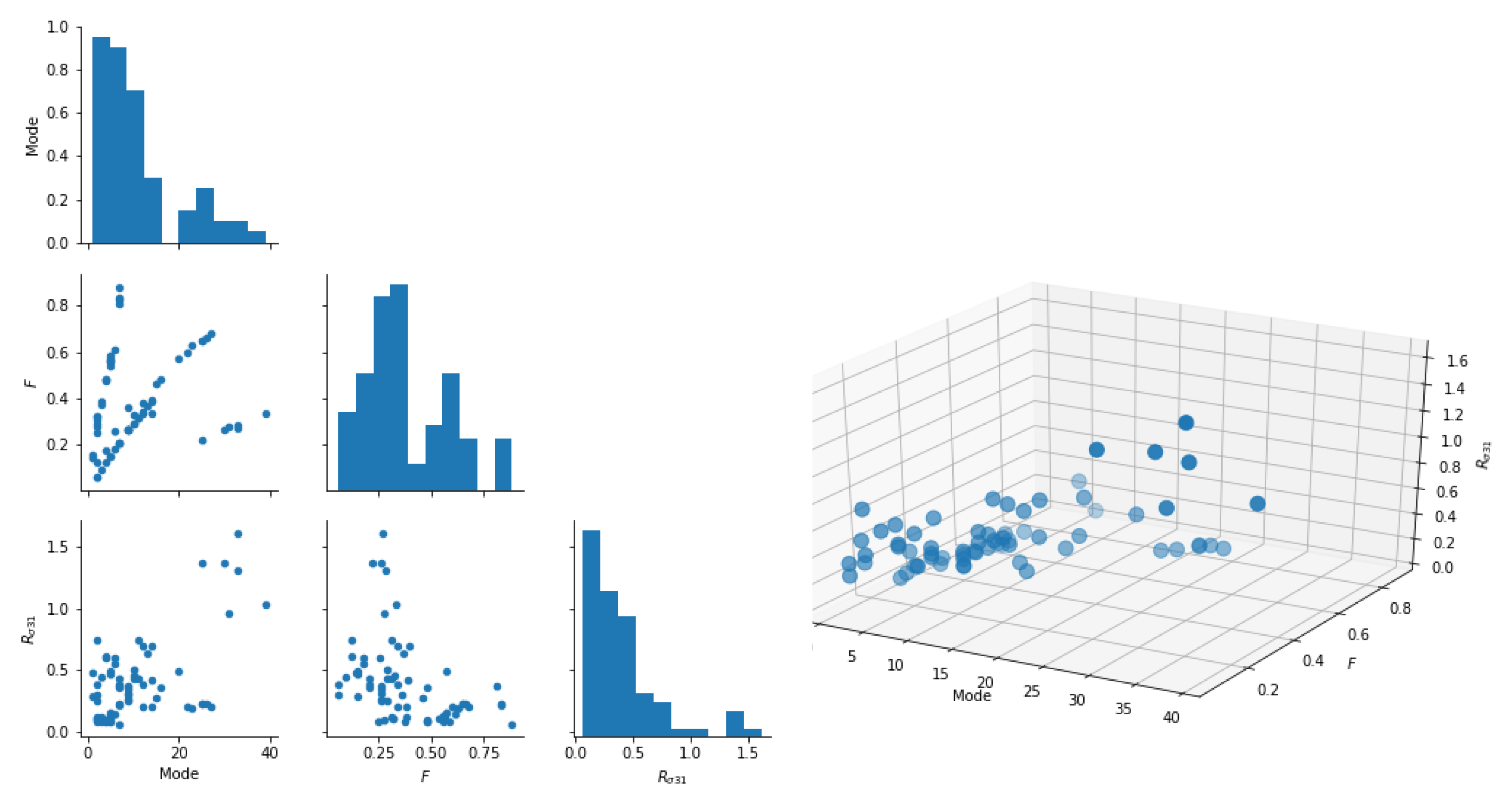
Instead of using one set of generalised parameters, we suggest clustering the model tests based on the physical response properties rather than the individual model test properties and to derive a set of parameters to be used with each cluster. The stress ratio ($R_{\sigma 31}$), bending stiffness ratio (F), and response mode number (n) are selected as inputs to the data clustering analysis as they seem to be good indicators of the different riser response characteristics (refer to Section 2). Consequently, they were selected for the clustering; their relative relations are shown in Figure 5. The outputs are clustered model test data.

These parameters are continuous, but as seen from Figure 5, they are not uniformly sampled by the model tests. We wish to identify clusters of similarity in the data under the assumption that the underlying distributions are continuous and any new model tests might close the gaps that at the moment seem to be obvious splits in the data. Consequently, we need a dynamic approach where the clustering can be easily adapted to new measurements and also expanded to include different/additional parameters.

In recent years, there has been a massive development of machine learning methods for clustering data based on similarities. Given the continuous nature of the parameters and possible overlap between clusters, conceptually different methods for clustering were tested and their performance compared. Based on the limited data sample presented here, they all perform similarly.

In the following, the application of various clustering methods is investigated. It is expected that the underlying distributions are continuous but can be represented as Gaussian distributions with additional overlaps due to the measurement uncertainties. The method of choice should be able to handle this. The presented clustering algorithms all require a fixed number of clusters to be pre-defined. In order to have a sufficiently high number of data points in the resulting clusters to derive the best-fit parameters, three clusters were used. As more data become available, the number of clusters should be adjusted. Before the data can be clustered it is customary to normalise all parameter values to the same numeric scale. This has been achieved with min–max-scaling: $x_{\mathrm{i}},\mathrm{scaled}=(x_i-x_{min})/(x_{max}-x_{min})$.

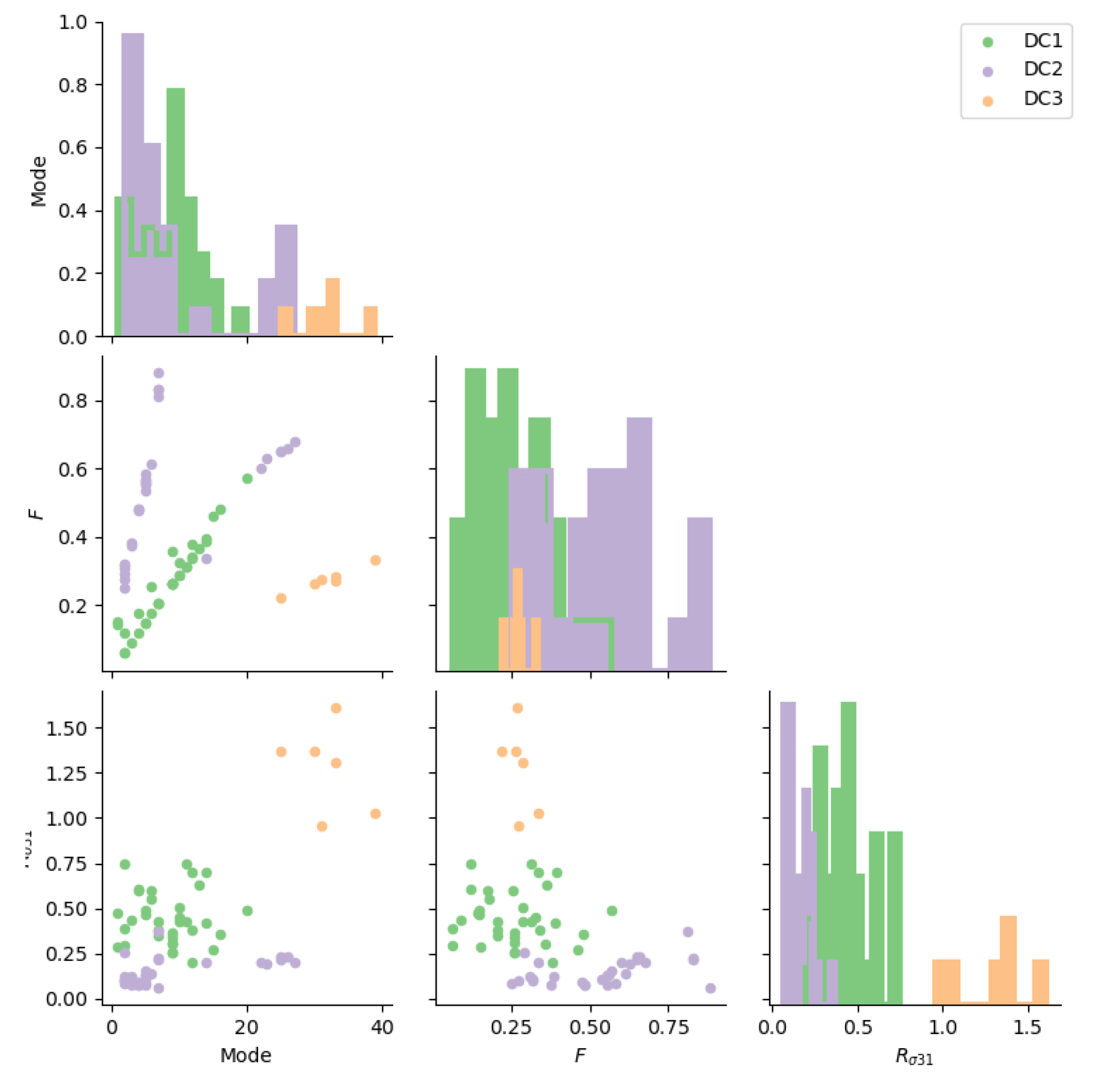
K means clustering [32] is a standard algorithm often used because of its simplicity. However, it does not cluster the data based on similarities but partitions the data into a user-defined number of chunks assumed to be spherical in the parameter space. This works well when the data consist of a known number of clearly separated clusters. However, the method is not very useful for deriving the number of clusters in a scenario with possible overlaps. The results from K means clustering are shown in Figure 6.

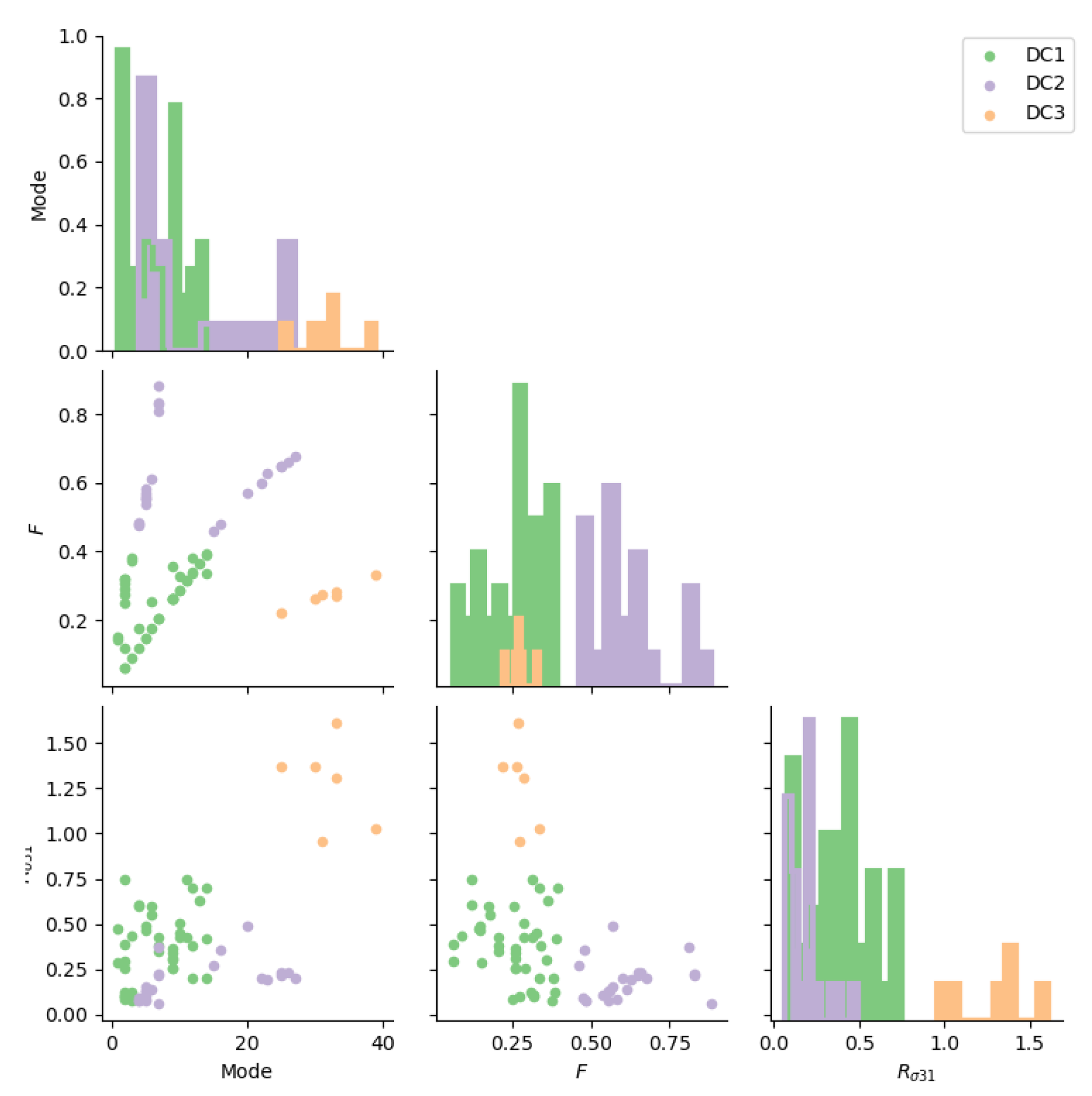
Gaussian Mixture [33,34,35] is a probabilistic model that assumes that all data points originate from a predetermined number of overlapping Gaussian distributions with unknown parameters. The results of Gaussian mixture clustering are shown in Figure 7.

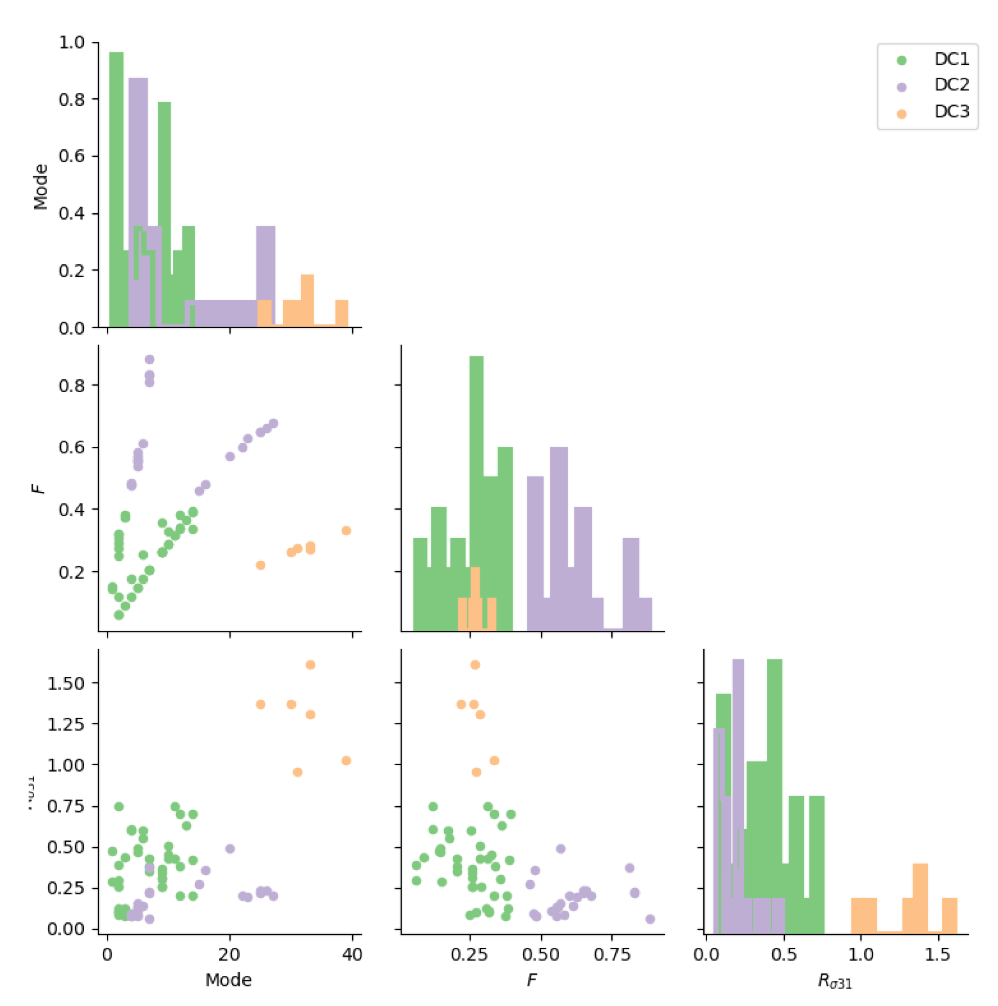
Spectral clustering [36,37] uses the spectrum (eigenvalues) of the similarity matrix of the data to reduce the number of dimensions before clustering in the low-dimension space. The number of clusters has to be specified, and it only works for a low number of clusters. The results of spectral clustering are shown in Figure 8.

As seen in Figure 6, Figure 7 and Figure 8, the different data clustering methods give very similar results for the parameter clustering, but they are not identical. The robustness of the clusters should be investigated with more data. The subsequent analysis was performed with the Gaussian mixture algorithm since the data are assumed to originate from continuous distributions of physical origin and can therefore be reasonably approximated with overlapping Gaussian distributions.

4.3. Identifying Response Characteristics by Data Clustering

In the present study, VIV response characteristics are represented by three parameters based on the five selected test data sets. The number of selected data points from various model tests and their allocations in three data clusters (DC 1–3) are reported in

Table 3. Results of Gaussian mixture clustering analysis.

Test	Number of Cases	DC1	DC2	DC3
NDP high-mode test	22	22	0	0
Shell high-mode test (pipe 2)	6	5	1	0
Hanøytangen	11	5	6	0
ExxonMobil rotating rig test	25	3	22	0
Miami II test	6	0	0	6

.

It can be seen from Table 3 that the data from the Hanøytangen test has been split into two roughly evenly sized groups associated with data clusters DC1 and DC2, respectively. In the Hanøytangen test, the structural stiffness for cases with a lower response mode (lower towing speeds) were tension-dominated. The response characteristics in terms of response magnitude and frequency contents are similar to Norwegian Deepwater Programme (NDP) and Shell tests. But the bending stiffness becomes dominant with increasing mode number. The response characteristics tend to be similar to the ExxonMobil test. The results from the clustering analysis agree with observations from the model tests. This illustrates the purpose of clustering analysis, which groups the cases with the same characteristics across different model tests. It is also shown in Figure 3 that it is difficult to use the bending stiffness ratio as one single parameter to cluster the data. The data from MIAMI showed significantly different behaviour as compared to other data with a similar bending stiffness ratio of about 0.3. The travelling speeds in CF and IL directions will be close due to its relatively low bending stiffness. In addition, the MIAMI model is responding at a very high mode, where the travelling wave response is dominating. Therefore, there is a long region along the length of the riser model where stable and favourable motion orbits are observed, which leads to high third-order stress as well as to high responses at the fundamental frequency. On the other hand, the other cases with similar or lower bending stiffness ratios have much lower third-order stress due to the motion orbits varying constantly along the length, which is caused by the presence of the standing waves at low response modes. The number of data groups is manually set to be 3 based on the data at hand. The clustering analysis correctly identified three clusters as requested. An optimal selection of the clusters will be expected when dealing with more complex data.

4.4. Obtaining Optimal Hydrodynamic Parameters

The excitation coefficient database is represented by a few parameters [4]. They are systematically varied until the prediction agrees with the measurement, as explained in [22]. The optimisation is carried out for each of the three data clusters. The mean squared error in fatigue damage has been used as the criterion to select the optimal parameters, i.e., ${\sum }_{i=1}^N{(Fa{t}_{pred,i}-Fa{t}_{meas,i})}^2/N$, where $i=1,2,3\dots N$, i is the sensor number along the length of the pipe. Two sets of hydrodynamic parameters have been derived, i.e., Ce1 and Ce2. Parameter set Ce1 was used to predict fatigue damage for cases in data cluster 1 (DC1), and the other set was used for data cluster 2 (DC2). No hydrodynamic parameters have been derived for data cluster 3 (DC3) due to the lack of experimental data time series from which to derive the parameters and to evaluate the fatigue damage. However, it is expected that a third set of hydrodynamic parameters is needed because the averaged displacement standard deviation of DC3 is indeed larger than that of the other data groups [38].

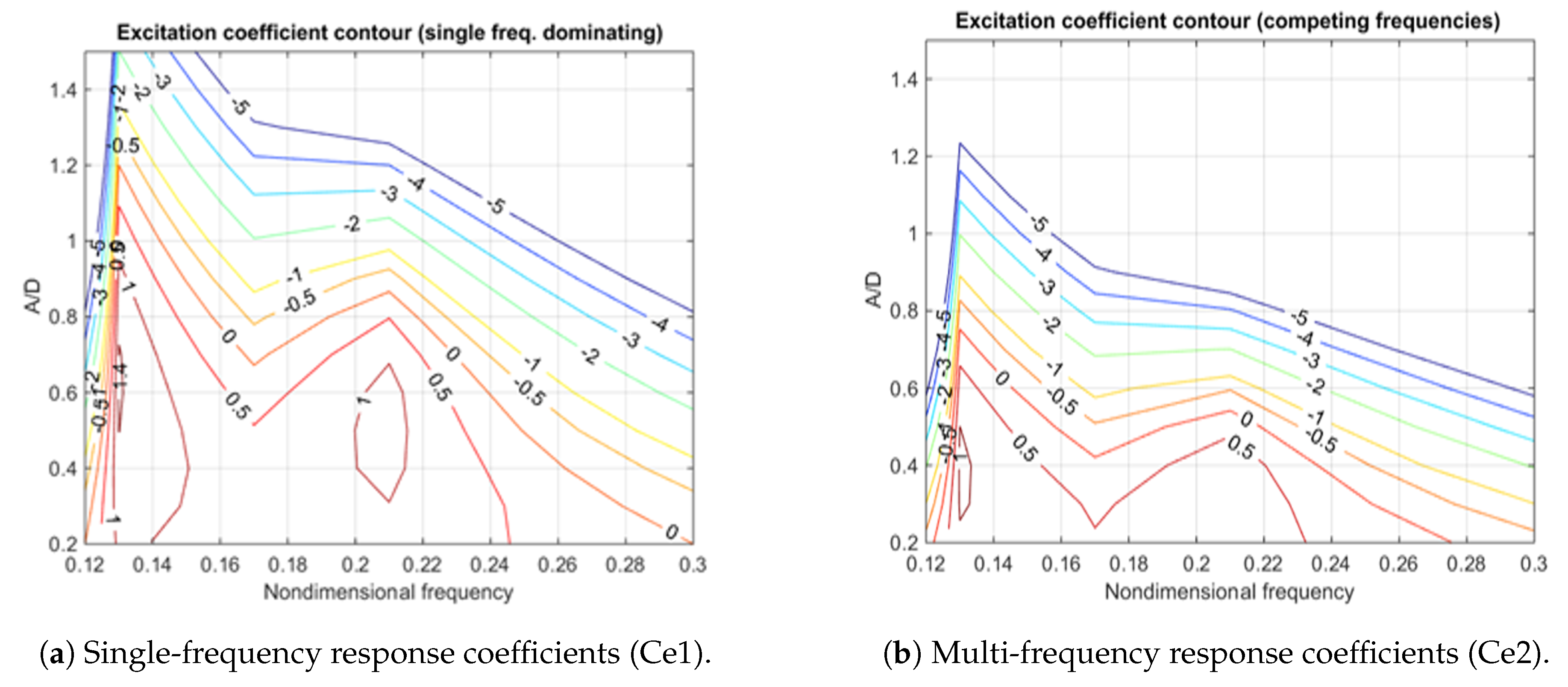
The reconstructed CF excitation coefficient contour plots are presented in Figure 9. The first set of parameters (Ce1), as represented by the force coefficient contour plot to the left, were developed in earlier studies [22]. This is representative for a tension-stiffness-dominated pipe dominated by a single response frequency. The second set of hydrodynamic parameters (Ce2), as shown in the plot to the right, is adjusted to represent the competing frequency responses of a bending-stiffness-dominated pipe.

4.5. Evaluating Prediction Accuracy

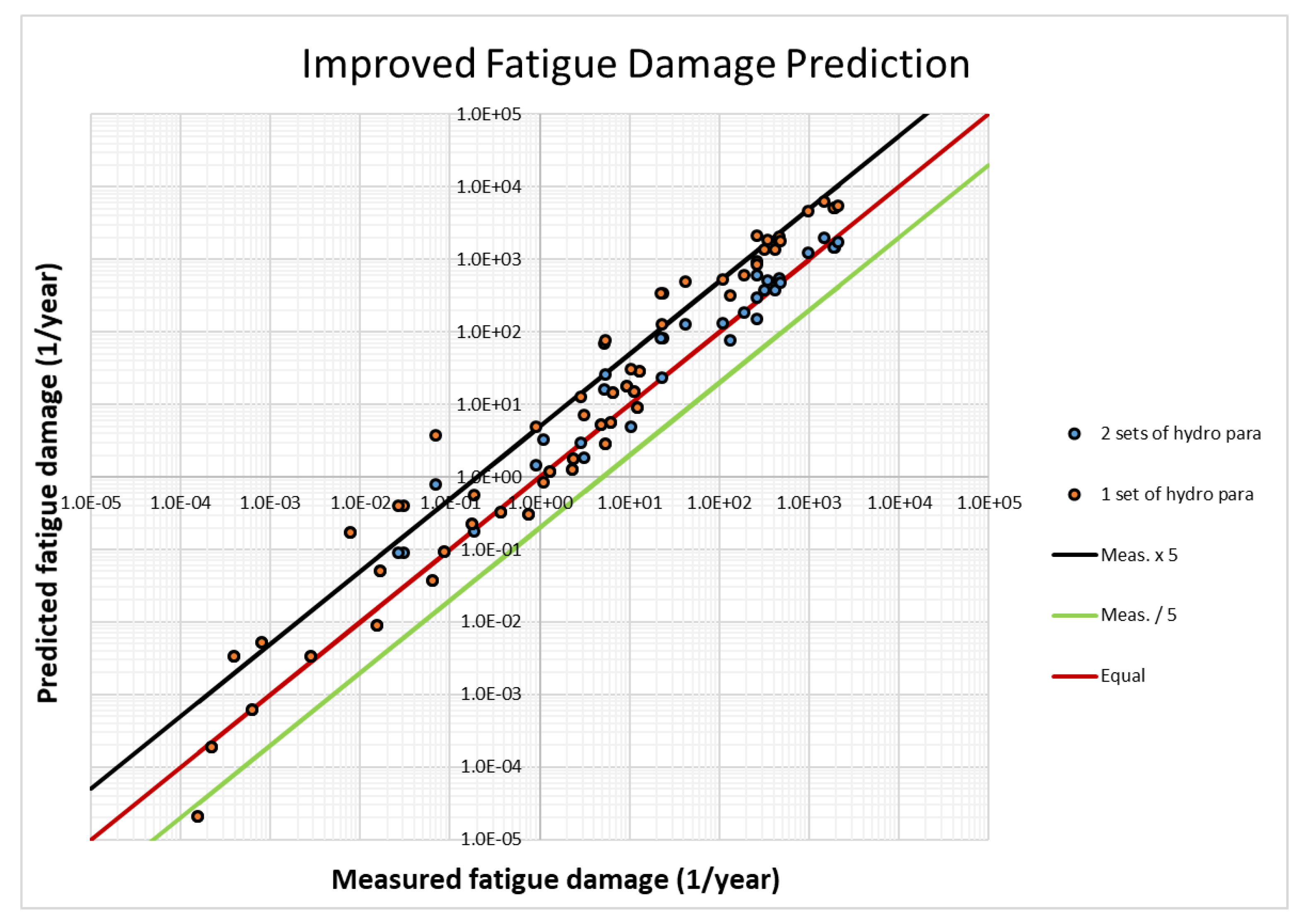
In Figure 10, the fatigue damage predictions of those cases for which a calculation with two sets of hydrodynamic parameters has been performed are compared to the respective predictions using only one parameter set. The red line indicates that the predicted fatigue damage is equal to the measured fatigue damage. The black lines show that the predicted fatigue damage is 5 times the measured value, and the green line shows that the predicted fatigue damage is 1/5 of the measured value. The narrower distribution along the diagonal obtained when using two sets of hydrodynamic parameters indicates a significant improvement in prediction accuracy. Only 7% of the predictions deviate by more than a factor of 5 from the measured fatigue damage, compared to 26% when using only one set of parameters. A prediction error within a factor of 3 is found in 86% of the cases, which represents an increase of 33% compared to the previous analysis with only one set of parameters.

4.6. Selection of Hydrodynamic Parameters for a New Data by Classification Algorithms

When new measurement data become available, the clustering model can be applied to determine which parameter sets should be used. Assuming a new test case with the following conditions: mode number of 25, bending stiffness ratio of 0.6, and stress ratio of 0.1. The developed Gaussian mixture model in Section 4.2 determines that this new data point will be classified to DC2, and consequently the best fitting parameters for DC2 should be applied to compute the fatigue.

The prediction accuracy needs to be evaluated and data re-clustering may be needed if the prediction accuracy is not satisfactory. New parameters may be identified and included in a new data clustering procedure. For example, the Reynolds number may be an additional clustering parameter when dealing with full-scale measurements [11,12].

5. Discussion

The novelty of the present work is to apply adaptive parameters in the prediction in order to account for the limitations of the simplified numerical models. The key element is to group the VIV responses and apply different hydrodynamic parameters for each individual response cluster. It is found to be increasingly difficult to derive analytical functions to describe the relationship among the increasing number of parameters. It is also not desirable to manually inspect the data, especially when the accumulation of data is large. Therefore, data clustering methods have been explored for grouping data in a multidimensional parameter space in the present study. For demonstration purposes, the strategy in the present work is to limit the scope to a relatively small data group as a first step. The data has been limited to selected laboratory tests with dense instrumentation with sheared current profiles. The good physical understanding of these limited cases provides a way to evaluate the use of the clustering analysis, which groups the data purely based on their similarities without physical meaning. Three parameters, i.e., stress ratio, stiffness ratio, and mode order (refer to Figure 3), were selected based on the physical understanding of the system. It is satisfactory to see that the clustering analysis leads to a similar selection of groups than otherwise could have been achieved manually. However, the ultimate goal is to eventually apply this concept for VIV predictions in riser design practice and for VIV field response monitoring, where increasing complexity in data quantity, quality, and physical systems are expected. Therefore, a more advanced clustering analysis is to be expected in practice.

More model test data need to be included in the analysis to increase the robustness of the parameter selection. More parameters are also needed in order to describe the characteristics of the riser response, e.g., the shape and direction of the flow profile, Reynolds number effect, etc. The clustering analysis will hopefully help to identify the indirect connections in the data in a multi-parameter space. Then, the improvement in modelling will be easier with the clear understanding of the limitations of the prediction tools. This process is also expected to be dynamic, which means that the improvement in the numerical models may potentially reduce the number of parameter sets otherwise required. This will be carried out step-wise so that the underlying physics are correctly understood.

The proposed concept can be applied to improve accuracy in riser design and in on-line response monitoring. While the stiffness ratio and even the mode order can be predicted, the stress ratio cannot be estimated beforehand. Eventually, other parameters will be used.

The geometry, operational, and environmental conditions of the riser systems in the field are much more complicated than in the laboratory tests. In addition, the field measurement quality and limited sensor density will introduce significant uncertainties. Field measurement data must be analysed to identify key parameters to describe response characteristics. These parameters and their values are not expected to be identical to those used in the design phase. But the knowledge gained from the analysis of laboratory data will provide a good basis for parameter selection and an understanding of the field observations. Learning from field measurements will certainly be valuable to improve the design basis as well.

6. Conclusions

A new analysis concept to improve VIV prediction accuracy by applying adaptive parameters has been proposed and demonstrated with simplified examples. The limitations of the mathematical model and the hydrodynamic parameters used in the existing perdition tools can be compensated by parameter optimisation based on groupings of the measured data. The identification and selection of these groups were determined adaptively by using data clustering algorithms. Improvement of both the prediction accuracy and consistency have been achieved. By using the adaptive parameter approach, 93% of the predictions are within a factor of 5 of the measured values, and 86% of the predictions are within a factor of 3 of the measured values. The corresponding percentages are 74% and 53% using original parameters.

The proposed analysis concept is semi-empirical, which means it is based on model test data. Enriching model test data will help increase the robustness of the parameters, so that the clustering analysis and VIV prediction will be improved. It is expected that the proposed analysis concept can be applied in both riser design and online riser response monitoring applications.

References

- Larsen, C.M.; Lie, H.; Passano, E.; Yttervik, R.; Wu, J.; Baarholm, G. VIVANA—Theory Manual Version 3.7; Technical Report; MARINTEK: Trondheim, Norway, 2009. [Google Scholar]
- Vandiver, J.K.; Li, L. Shear7 v4.5 Program Theoretical Manual; Massachusetts Institute of Technology: Cambridge, MA, USA, 2007. [Google Scholar]
- Triantafyllou, M.; Triantafyllou, G.; Tein, Y.D.; Ambrose, B.D. Pragmatic Riser VIV Analysis. In Proceedings of the Offshore Technology Conference, Houston, TX, USA, 3–6 May 1999. Number OTC-10931-MS. [Google Scholar]
- Gopalkrishnan, R. Vortex-Induced Forces on Oscillating Bluff Cylinders. Ph.D. Thesis, Massachusetts Institute of Technology, Cambridge, MA, USA, 1993. [Google Scholar]
- Aronsen, K.H. An Experimental Investigation of In-line and Combined In-line and Cross-flow Vortex Induced Vibrations. Ph.D. Thesis, Norwegian University of Science and Technology, Trondheim, Norway, 2007. [Google Scholar]
- Dahl, J.M. Vortex-Induced Vibration of a Circular Cylinder with Combined In-line and Cross-flow Motion. Ph.D. Thesis, Center for Ocean Engineering, Department of Mechanical Engineering, MIT, Webb Institudte, Glen Cove, NY, USA, 2008. [Google Scholar]
- Zheng, H.; Price, R.; Modarres-Sadeghi, Y.; Triantafyllou, G.S.; Triantafyllou, M.S. Vortex-Induced Vibration Analysis (VIVA) Based on Hydrodynamic Databases. In Proceedings of the ASME 2011 30th International Conference on Ocean, Offshore and Arctic Engineering, Rotterdam, The Netherlands, 19–24 June 2011; Volume 7, pp. 657–663. [Google Scholar]
- Yin, D. Experimental and Numerical Analysis of Combined In-line and Cross-flow Vortex-Induced Vibrations. Ph.D. Thesis, Norwegian University of Science and Technology, Trondheim, Norway, 2013. [Google Scholar]
- Aglen, I.M. VIV in Free Spanning Pipelines. Ph.D. Thesis, Norwegian University of Science and Technology, Trondheim, Norway, 2013. [Google Scholar]
- Ding, Z.J.; Balasubramanian, S.; Lokken, R.T.; Yung, T.W. Lift and damping characteristics of bare and straked cylinders at riser scale Reynolds numbers. In Proceedings of the Offshore Technology Conference; Offshore Technology Conference, Houston, TX, USA, 3–6 May 2004. [Google Scholar]
- Lie, H.; Szwalek, J.L.; Russo, M.; Braaten, H.; Baarholm, R.J. Drilling riser VIV tests with prototype Reynolds numbers. In Proceedings of the ASME 2013 32nd International Conference on Ocean, Offshore and Arctic Engineering, Nantes, France, 9–14 June 2013; Volume 7, p. V007T08A086. [Google Scholar]
- Yin, D.; Lie, H.; Baarholm, R.J. Prototype Reynolds number VIV tests on a full-scale rigid riser. ASME. J. Offshore Mech. Arct. Eng. 2018, 140, 011702. [Google Scholar] [CrossRef]
- Trim, A.; Braaten, H.; Lie, H.; Tognarelli, M. Experimental investigation of vortex-induced vibration of long marine risers. J. Fluids Struct. 2005, 21, 335–361. [Google Scholar] [CrossRef]
- Huse, E.; Kleiven, G.; Nielsen, F. Large scale model testing of deep sea risers. In Proceedings of the Offshore Technology Conference, Houston, TX, USA, 4–7 May 1998. [Google Scholar]
- Vandiver, J.K.; Jaiswal, V.; Jhingran, V. Insights on vortex induced, traveling waves on long risers. J. Fluids Struct. 2009, 25, 641–653. [Google Scholar] [CrossRef]
- Nielsen, F.G.; Søreide, T.H.; Kvarme, S.O. VIV Response of Long Free Spanning Pipelines. In Proceedings of the ASME 2002 21st International Conference on Offshore Mechanics and Arctic Engineering, Oslo, Norway, 23–28 June 2002. [Google Scholar]
- Lie, H.; Braaten, H.; Kristiansen, T.; Nielsen, F.G. Free-Span VIV Testing Of Full-Scale Umbilical. In Proceedings of the Seventeenth International Offshore and Polar Engineering Conference, Lisbon, Portugal, 1–6 July 2007. [Google Scholar]
- Lie, H.; Mo, K.; Vandiver, J.K. VIV Model Test of a Bare- and a Staggered Buoyancy Riser in a Rotating Rig. In Proceedings of the Offshore Technology Conference, Houston, TX, USA, 4–7 May 1998. Number OTC8700. [Google Scholar]
- Chaplin, J.; Bearman, P.; Huarte, F.H.; Pattenden, R. Laboratory measurements of vortex-induced vibrations of a vertical tension riser in a stepped current. J. Fluids Struct. 2005, 21, 3–24. [Google Scholar] [CrossRef]
- Wu, J.; Maincon, P.; Larsen, C.M.; Lie, H. VIV force identification using classical optimal control algorithm. In Proceedings of the ASME 2009 28th International Conference on Ocean, Offshore and Arctic Engineering, Honolulu, HI, USA, 31 May 5–June 2009. [Google Scholar]
- Wu, J.; Larsen, C.M.; Lie, H. Estimation of hydrodynamic coefficients for VIV of slender beam at high mode orders. In Proceedings of the ASME 2010 29th International Conference on Ocean, Offshore and Arctic Engineering, Shanghai, China, 6–11 June 2010. [Google Scholar]
- Voie, P.; Wu, J.; Larsen, C.; Resvanis, T.; Vandiver, K.; Triantafyllou, M. Consolidated guideline on analysis of vortex-induced vibrations in risers and umbilicals. In Proceedings of the ASME 2017 36th International Conference on Ocean, Offshore and Arctic Engineering, Trondheim, Norway, 25–30 June 2017. [Google Scholar]
- Campbell, M.; Tognarelli, M. Drilling Riser VIV: Fact or Fiction? In Proceedings of the IADC/SPE Drilling Conference and Exhibition, Orleans, LA, USA, 2–4 February 2010. [Google Scholar]
- Riemer-Sørensen, S.; Wu, J.; Lie, H.; Savik, S.; Kim, S. Data-driven prediction of vortex-induced vibration response of marine risers subjected to three-dimensional current. Norwegian AI Society Symposium, Trondheim, Norway, 27–28 May 2019. [Google Scholar]
- Bourguet, R.; Karniadakis, G.E.; Triantafyllou, M.S. Distributed lock-in drives broadband vortex-induced vibrations of a long flexible cylinder in shear flow. J. Fluid Mech. 2013, 717, 361–375. [Google Scholar] [CrossRef] [Green Version]
- Wu, J.; Yin, D.; Lie, H.; Larsen, C.M.; Baarholm, R.J.; Liapis, S. On the Significance of the Higher-Order Stress in Riser Vortex-Induced Vibrations Responses. J. Offshore Mech. Arct. Eng. 2018, 141, 011705. [Google Scholar] [CrossRef]
- Larsen, C.M.; Zhao, Z.; Lie, H. Frequency Components of Vortex Induced Vibartions in Sheared Current. In Proceedings of the ASME 2012 31st International Conference of Ocean, Offshore and Arctic Engineering, Rio de Janeiro, Brazil, 1–6 July 2012. [Google Scholar]
- Swithenbank, S.B. Dynamics of Long Flexible Cylinders at High-Mode Number in Uniform and Sheared Flows. Ph.D. Thesis, Massachusetts Institute of Technology, Cambridge, MA, USA, 2007. [Google Scholar]
- Voie, P.E.; Larsen, C.M.; Wu, J.; Resvanis, T. Guideline on Analysis of Vortex-Induced Vibrations; Technical Report 2016-0226, Rev. 0; Statoil Petroleum AS: Stavanger, Norway, 2016. [Google Scholar]
- Wu, J.; Lie, H.; Larsen, C.M.; Liapis, S.; Baarholm, R. Vortex-induced vibration of a flexible cylinder: Interaction of the in-line and cross-flow responses. J. Fluids Struct. 2016, 63, 238–258. [Google Scholar] [CrossRef]
- Mukundan, H.; Chasparis, F.; Hover, F.S.; Triantafyllou, M.S. Optimal lift force coefficient databases from riser experiments. J. Fluids Struct. 2010, 26, 160–175. [Google Scholar] [CrossRef]
- Lloyd, S. Least squares quantization in PCM. IEEE Trans. Inf. Theory 1982, 28, 129–137. [Google Scholar] [CrossRef]
- Bishop, C. Pattern Recognition and Machine Learning; Information Science and Statistics; Springer: New York, NY, USA, 2006. [Google Scholar]
- Attias, H. A variational baysian framework for graphical models. Adv. Neural Inf. Process. Syst. 2000, 209–215. [Google Scholar]
- Blei, D.M.; Jordan, M.I. Variational inference for Dirichlet process mixtures. Bayesian Anal. 2006, 1, 121–143. [Google Scholar] [CrossRef]
- Shi, J.; Malik, J. Normalized Cuts and Image Segmentation. IEEE Trans. Pattern Anal. Mach. Intell. 2000, 22. [Google Scholar] [CrossRef] [Green Version]
- Luxburg, U.V. A Tutorial on Spectral Clustering. Stat. Comput. 2007, 17, 395–416. [Google Scholar] [CrossRef]
- Swithenbank, S.B.; Vandiver, J.K.; Larsen, C.M.; Lie, H. Reynolds number dependence of flexible cylinder VIV response data. In Proceedings of the ASME 2008 27th International Conference on Ocean, Offshore and Arctic Engineering, Estoril, Portugal, 15–20 June 2008; Volume 5, pp. 503–511. [Google Scholar]
- Lie, H.; Braaten, H.; Jhingran, V.; Sequeiros, O.E.; Vandiver, J.K. Comprehensive Riser VIV Model Tests in Uniform and Sheared Flow. In Proceedings of the 31st International Conference on Ocean, Offshore and Arctic Engineering, Rio de Janeiro, Brazil, 1–6 July 2012. [Google Scholar]
- Tognarelli, M.; Slocum, S.; Frank, W.; Campbell, R.B. VIV Response of a Long Flexible Cylinder in Uniform and Linearly Sheared Currents. In Proceedings of the Offshore Technology Conference, Houston, TX, USA, 3–6 May 2004. [Google Scholar]
© 2020 by the authors. Licensee MDPI, Basel, Switzerland. This article is an open access article distributed under the terms and conditions of the Creative Commons Attribution (CC BY) license (http://creativecommons.org/licenses/by/4.0/).