Photogrammetry: Linking the World across the Water Surface


Abstract
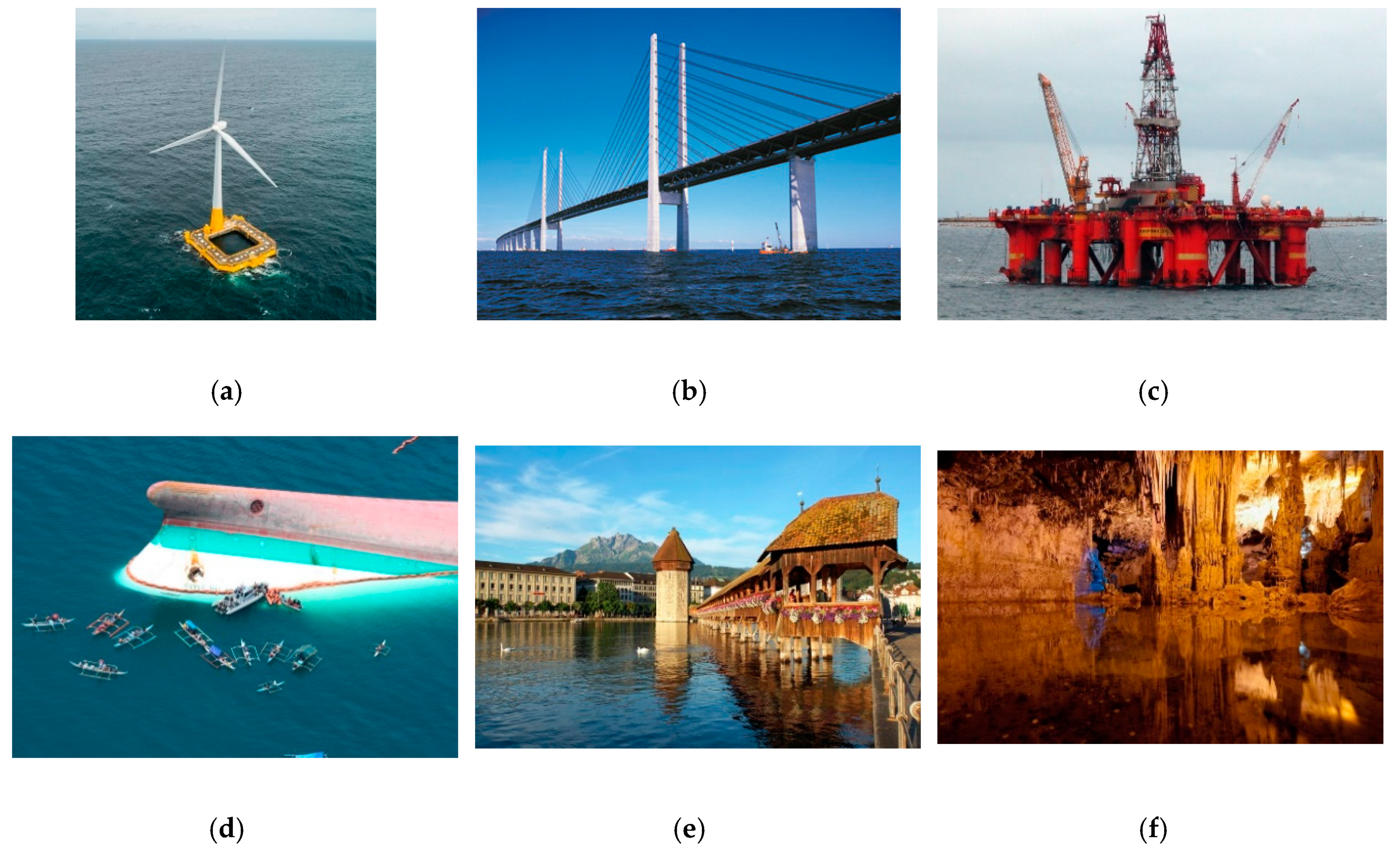
:1. Introduction
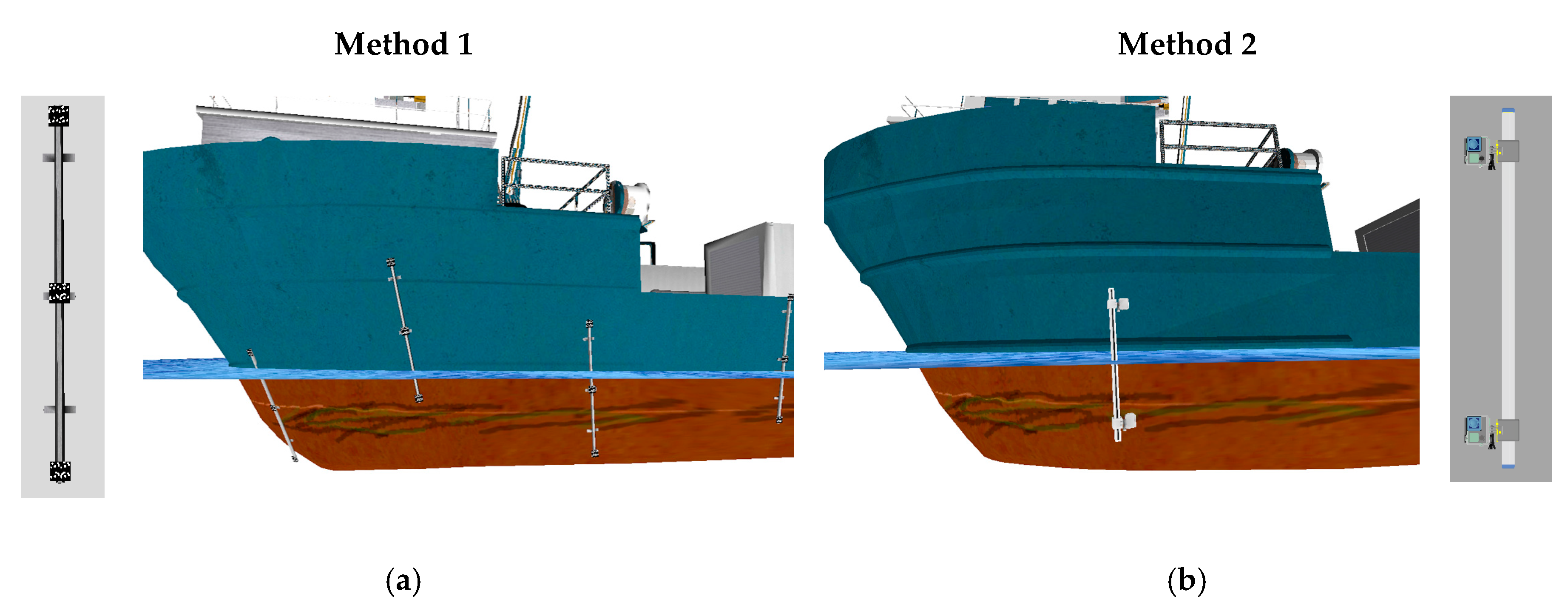
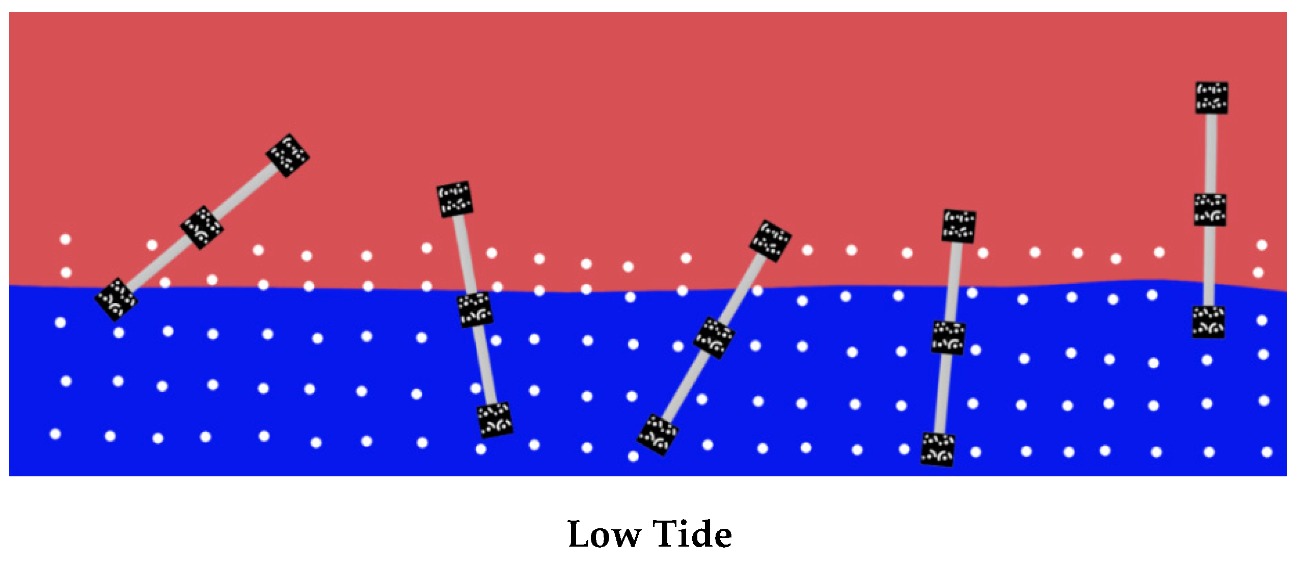
- Using rigid pre-calibrated rods installed across the waterline on the object to be surveyed;
- Using a synchronized underwater stereo-camera rig.
- The theoretical framework for two different possible approaches has been unified;
- The processing of the Costa Concordia survey has been updated and refined, following a fully automatic pipeline which merges the advantages of state-of-the-art structure from motion (SfM) – multi view stereo (MVS) procedures with the rigorousness of photogrammetry; moreover, the results of the newly implemented independent model adjustment to link the part below the water with the part above the water are reported for the first time;
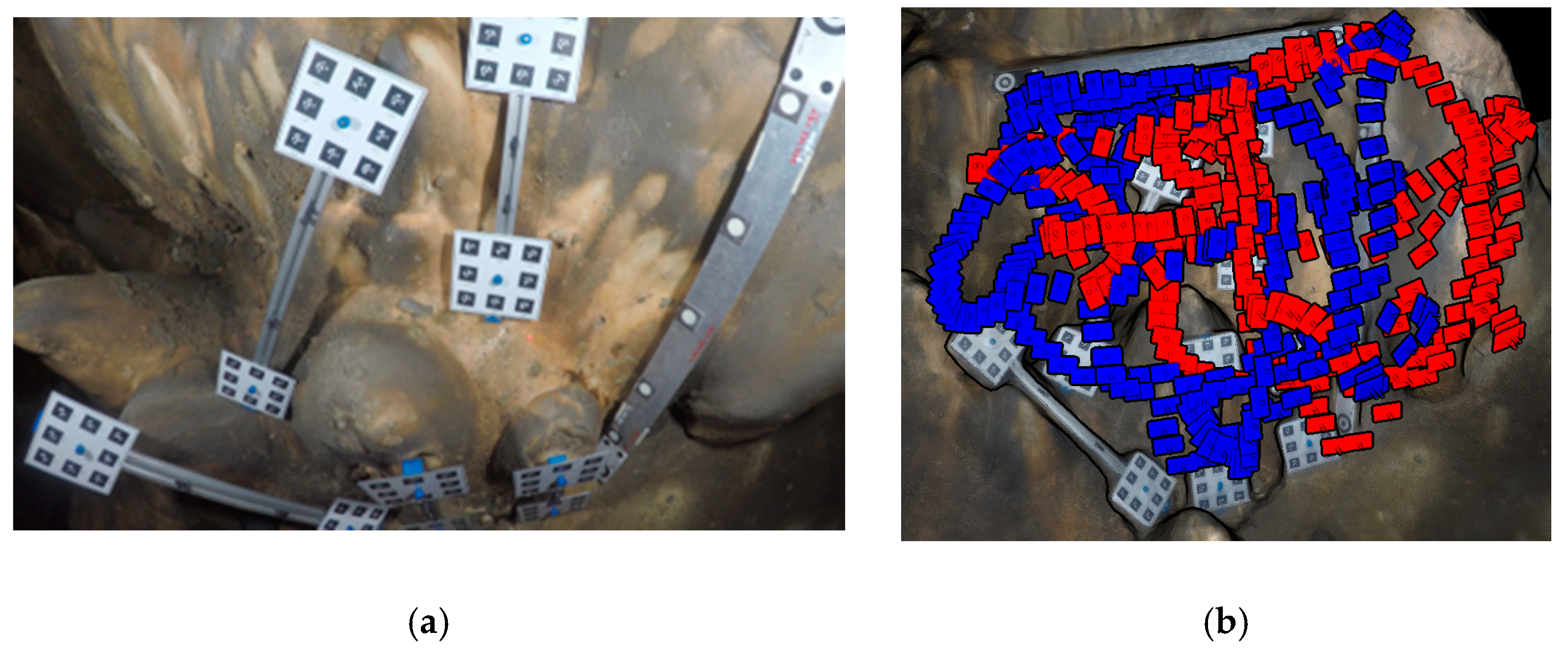
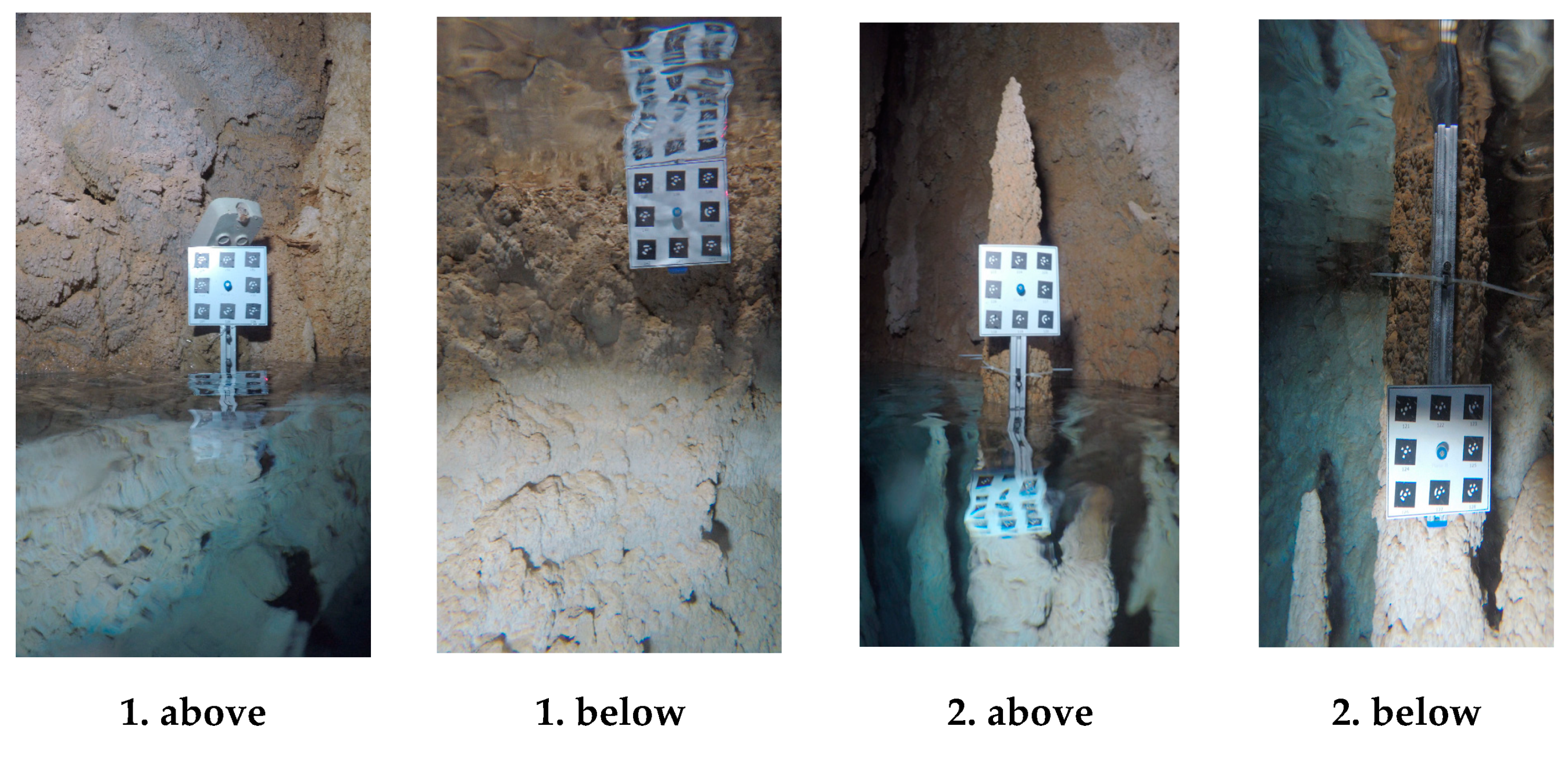
- Details of the relative orientation procedure for joining the above and underwater surveys of the ‘Grotta Giusti’ semi-submerged cave system based on a synchronized stereo camera are reported and discussed.
2. Materials and Methods
2.1. Overview of the Two Methods
- An underwater photogrammetry survey of the submerged part;
- An above the water photogrammetric survey of the emerged part;
- An optimized analytical process to link the two photogrammetric coordinate systems together for a seamless 3D model generation.
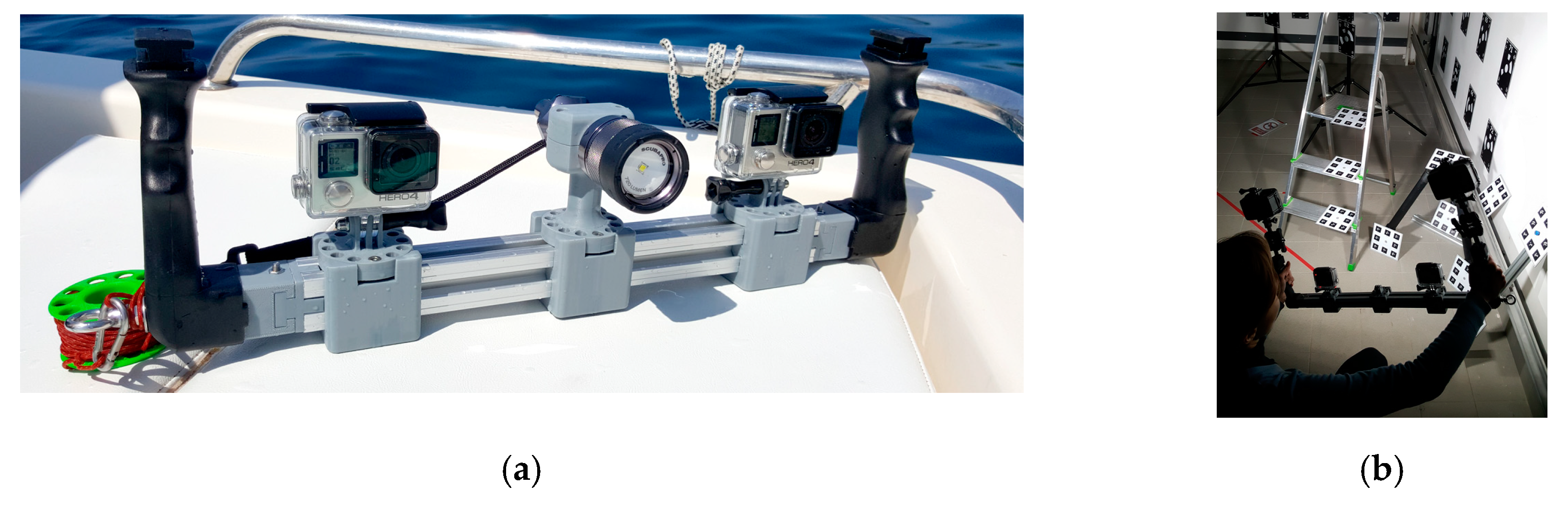
2.2. Method 1 Precalibrated Linking Targets
- Each single linking target is roto-translated, one at time, through a rigid similarity transformation and the target coordinates of the rod plates are determined in each of the two photogrammetric models (Figure 3a,b);
- The two photogrammetric models of the above and underwater parts are oriented in the same coordinate system, choosing one of the them as reference;
- In the last step, a refinement of the alignment is performed by re-computing simultaneously the similarity transformations for the models and the coordinates of all the target plates on the rods (Figure 3c).
2.2.1. Coarse Alignment between the Two Photogrammetric Models
- being the target, global, reference, or higher-order coordinate system, i.e., the final coordinate system where the coordinates of the points must be known;
- being the local or lower-order coordinate system, i.e., the initial coordinate system where the coordinates of the points have been measured.
- are the coordinates of a generic point P in the target system (here the apex indicates the system where the coordinates are defined);
- are the coordinates of the origin of system known into system ;
- is the diagonal matrix containing the scale factors in the three directions; usually , i.e., an isotropic scale factor exists between the two systems so that reduces to:
- is the 3 × 3 rotation matrix from system to system :where and and are the three rotation angles between the two coordinate systems. It is noteworthy that the rotation matrix contains the sequential rotations that, applied to the axes of target system , transform system to be parallel with system :
- are the coordinates of point P in system .
- and are the homogeneous coordinates of point P with respect to system and system , respectively;
- the transformation matrix is given by:being the elements of the rotation matrix (3) .
2.2.2. Refinement of the Alignment through Independent Models Adjustment
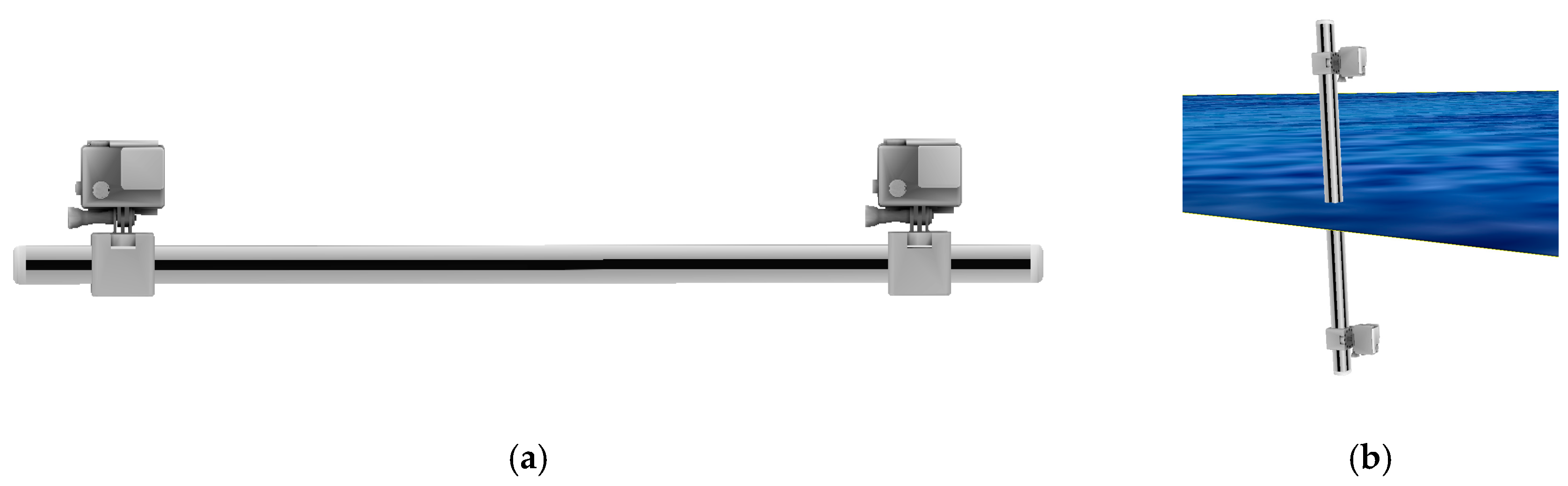
2.3. Method 2 Precalibrated Stereo Camera
3. Results
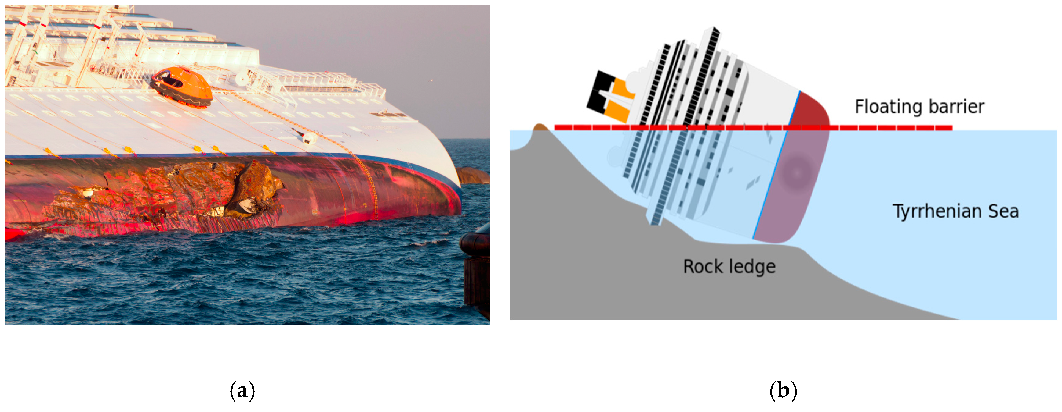
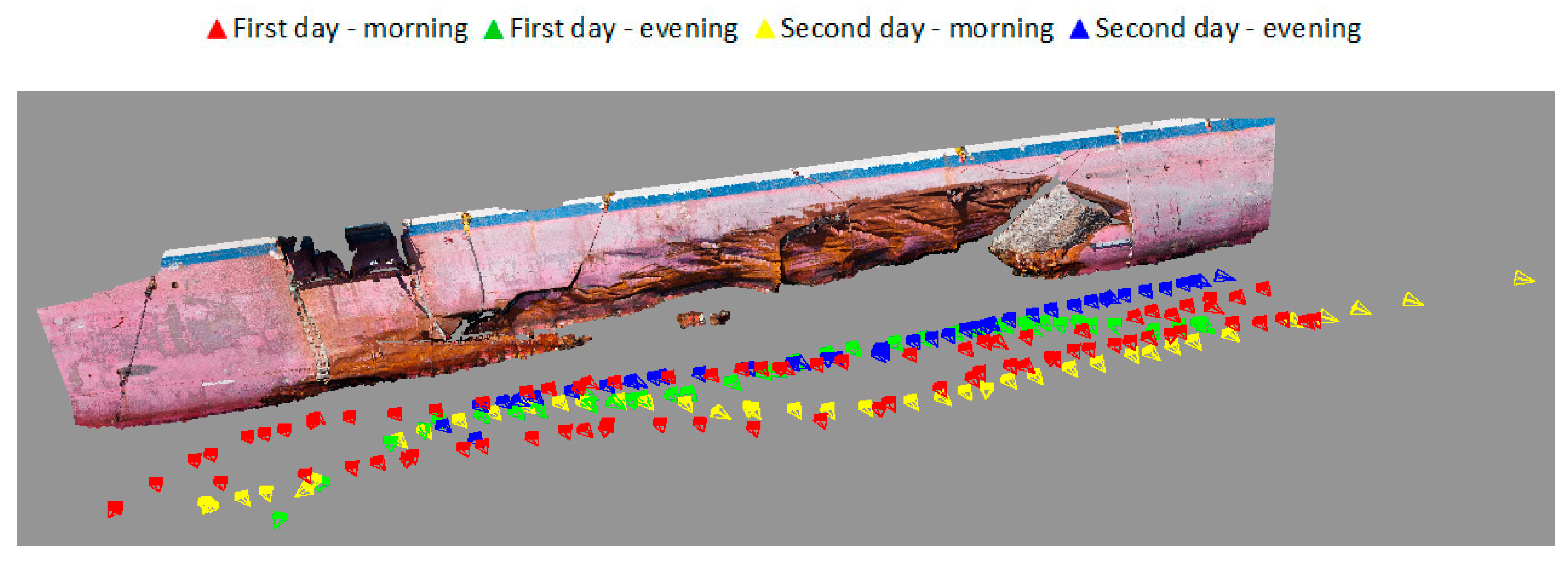
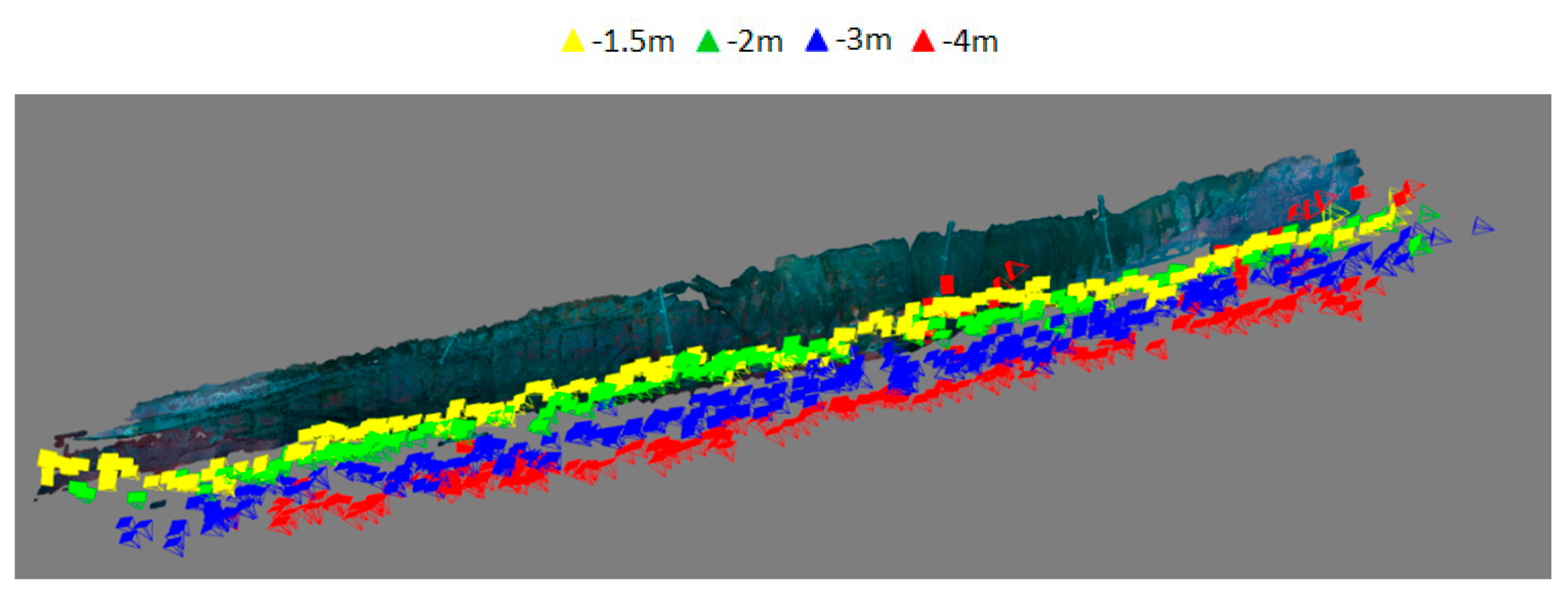
3.1. Case Study 1: Photogrammetric Survey of Semi-Submerged Object Using Linking Targets on Pre-Calibrated Rods. The Case Study of Costa Concordia Shipwreck
- -
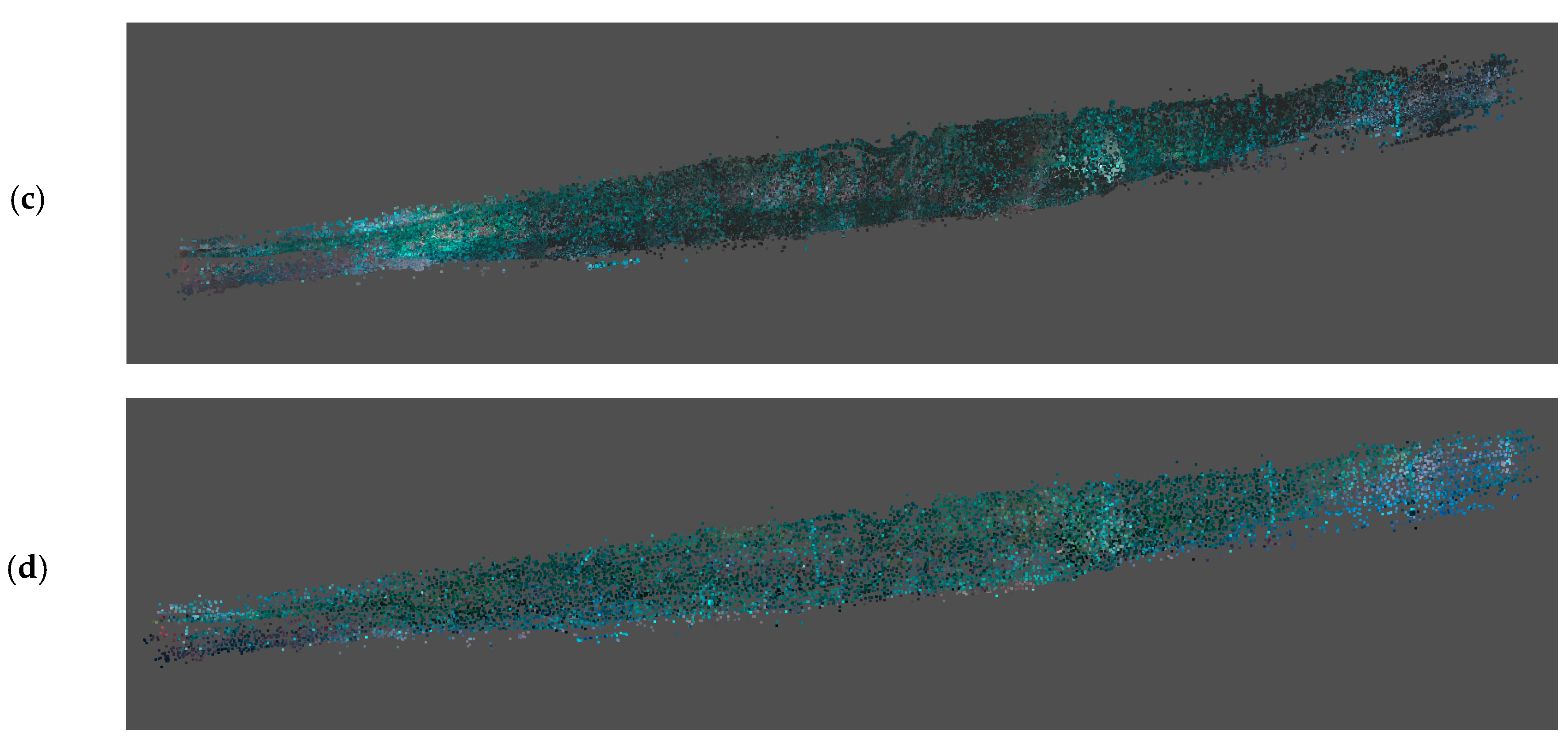
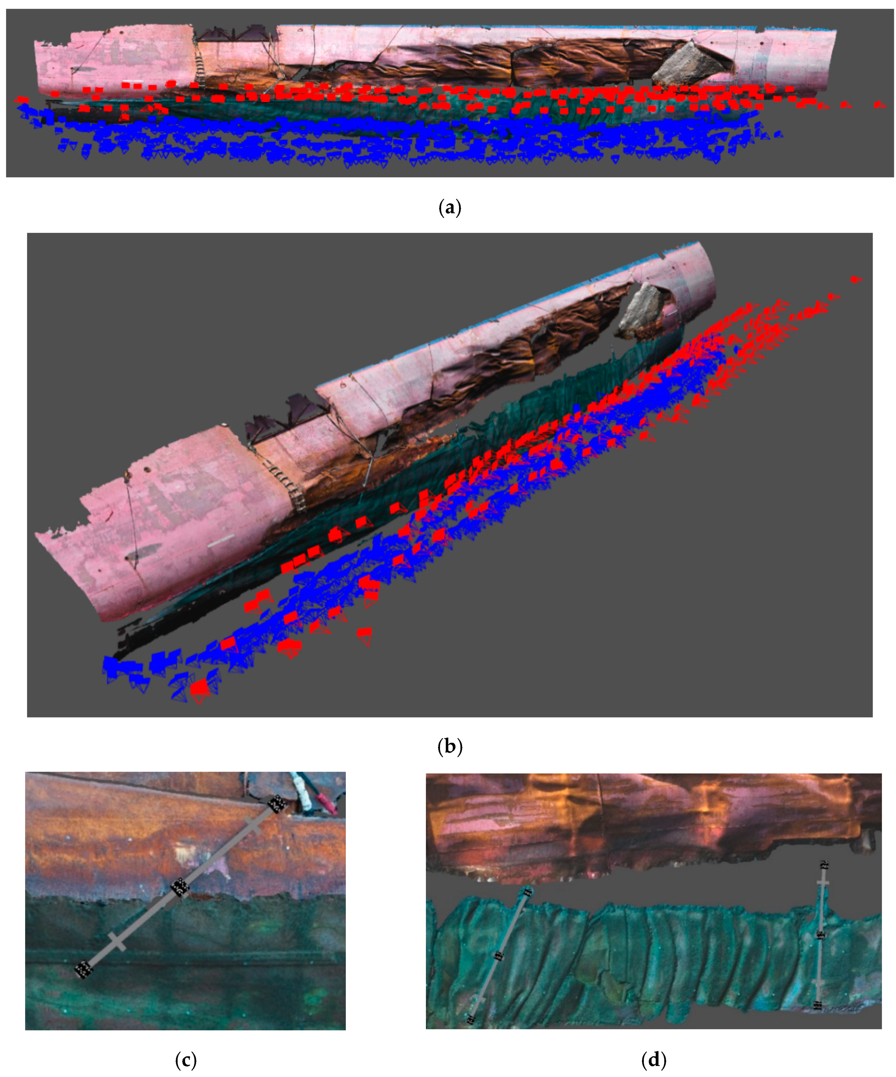
- Four strips were realized at different planned depths (namely −1.5 m, −2 m, −3 m, and −4 m) in different days. In Figure 9 the separate strips at different depths are displayed in different colors;
- -
- The shots were taken to assure a forward overlap of circa 80% (50 cm distance along strip) and a sidelap of circa 40% between two adjacent strips
- -
- A mean distance of circa 3 m was maintained from the hull in order to assure the necessary GSD and a sufficient contrast on the hull surface according to the average visibility ascertained after a preliminary underwater reconnaissance.
- Automatic image orientation and triangulation using structure from motion (SfM) tools.
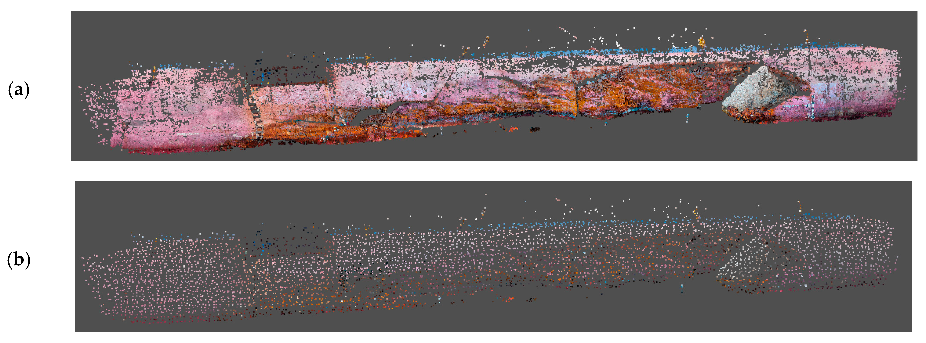
- Filtering and regularization of automatic extracted tie points: a filtering and regularization procedure of tie points from SfM algorithms was developed and tested in several applications and presented in previous papers [20,22]. The leading principle of the procedure is to regularize the distribution of tie points in object space, while preserving connectivity and high multiplicity between observations. A regular volumetric grid (voxelization) is generated, and the side length of each voxel is set equal to a fixed percentage of the image footprint and decided in order to guarantee a redundant number of observations in each image. The 3D tie points that are inside each voxel are collected in a subset. A score is assigned to each point on the basis of the following properties listed in ascending order of importance: (i) point’s proximity to the barycenter of the considered voxel, (ii) point’s visibility on more than two images, (iii) intersecting angle, (iv) point’s visibility on images belonging to different blocks or strips. The 3D tie points with the highest score in each cell are kept. The results of the filtering are shown in Figure 10 and summarized in Table 1 and Table 2.
- Photogrammetric bundle adjustment using the filtered tie points as image observations: different versions of self-calibrating bundle adjustment were run, separately for the emerged and submerged models. All the strips were processed following both (a) a free network adjustment with a-posteriori scaling (using both the scale bars and the visible parts of the rods) and (b) using the same reference distances as constraints in the adjustment process. For the above-the-water mode, a further test was considered, using only the closest strips carried out in the evening, hence with very similar lighting conditions and almost simultaneous with the underwater surveys and the known distances as constraints. The combination providing the best independent model adjustment was selected, i.e., the constrained adjustment with only the closest strips for the above-the-water model and constrained adjustment with all the strips for the underwater model. Their results are summarized in Table 3.
- Dense image matching: the exterior, interior orientation and additional parameters obtained from the photogrammetric bundle adjustment of the two surveys were used for the generation of separate high dense point clouds (Figure 11).
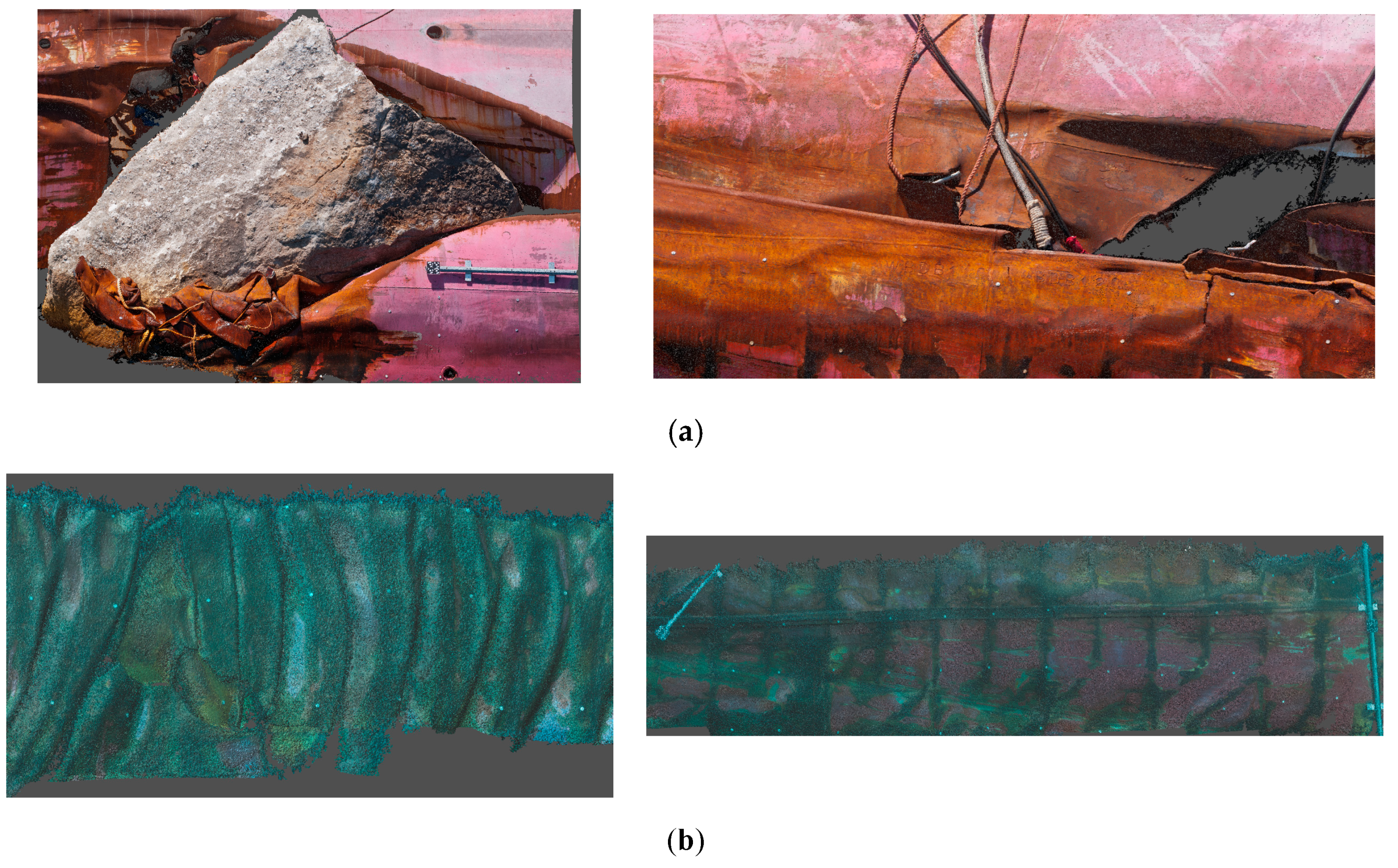
- Mesh generation and editing: The two high dense point clouds were finally triangulated using the Poisson algorithm [34] implemented in CloudCompare [33]. The optimization procedure described in [35] was used to find the optimum compromise between resolution and usability of the generation of meshes useful for successive analyses, such as highlighting of cracks, calculation of the water flood through the leak, etc. [10].
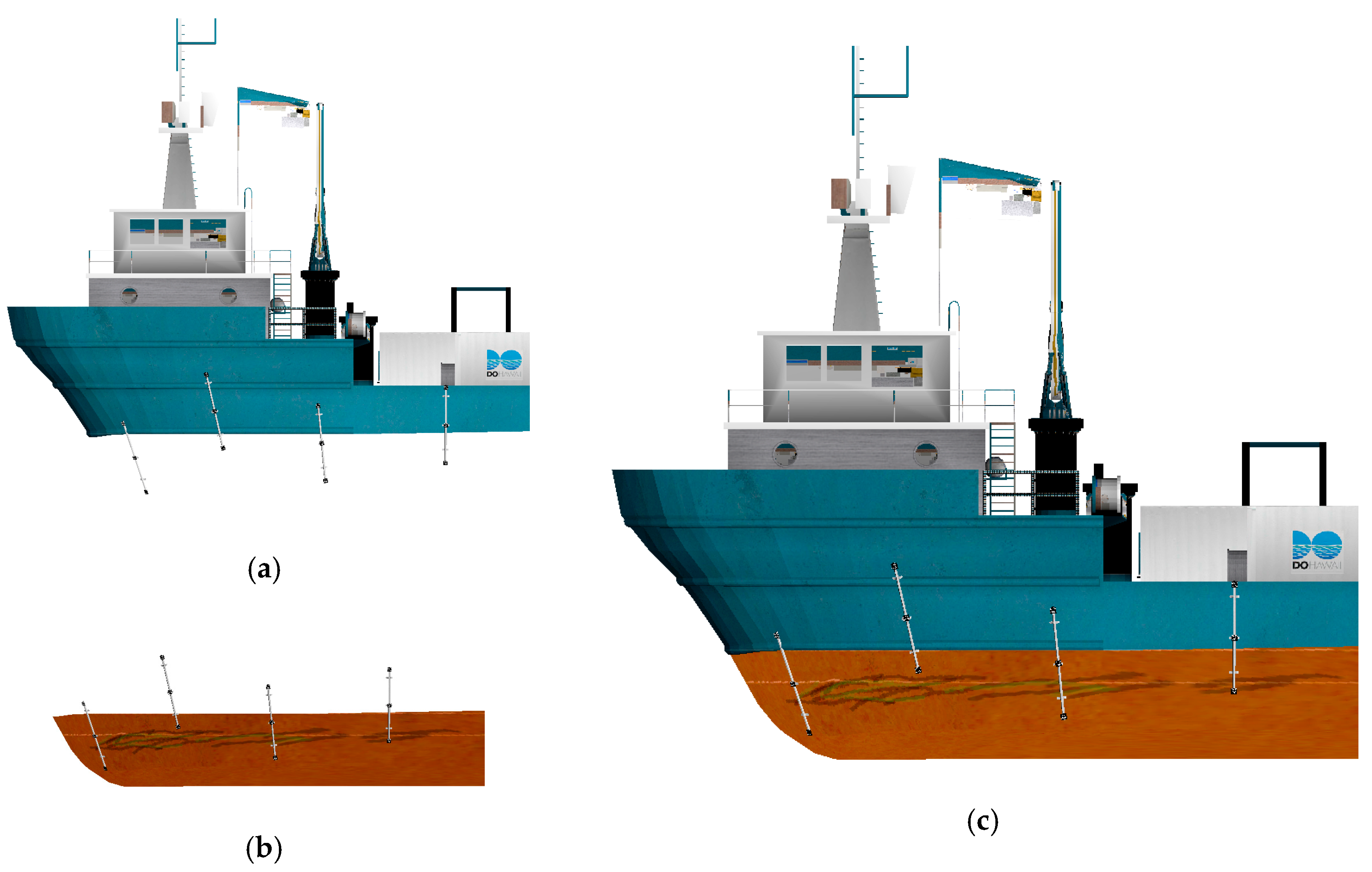
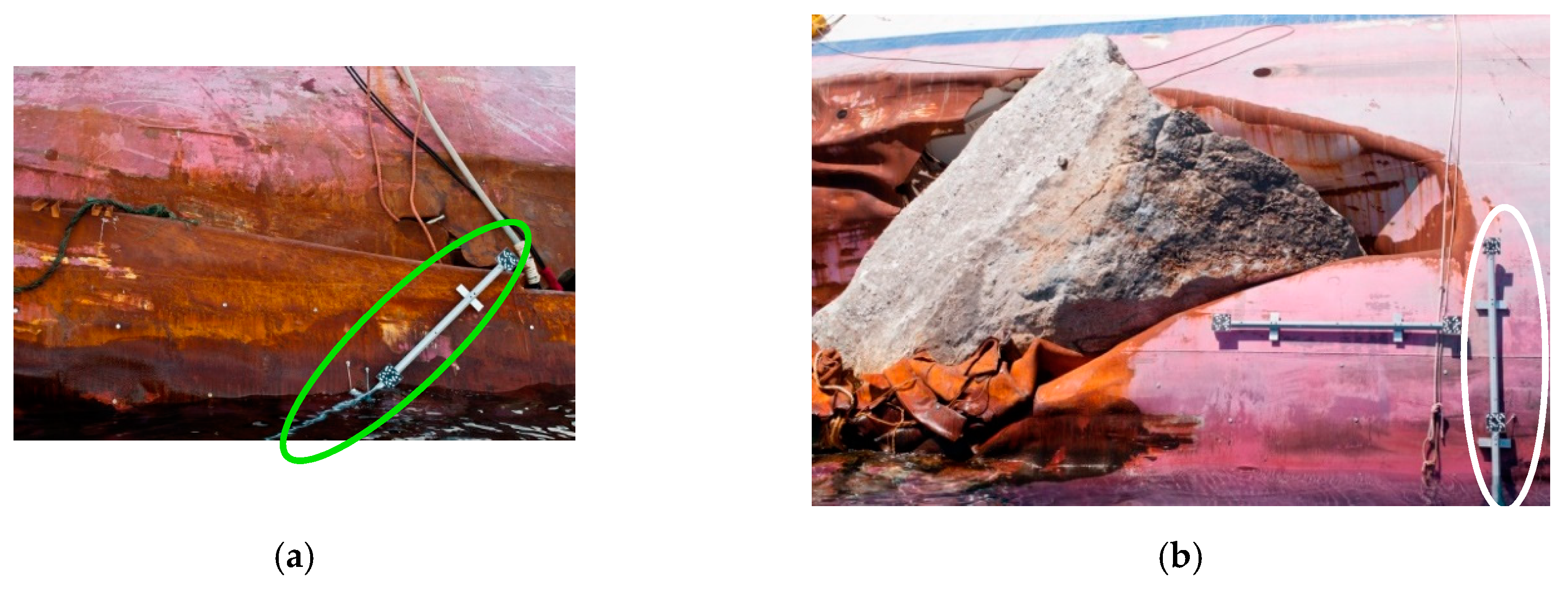
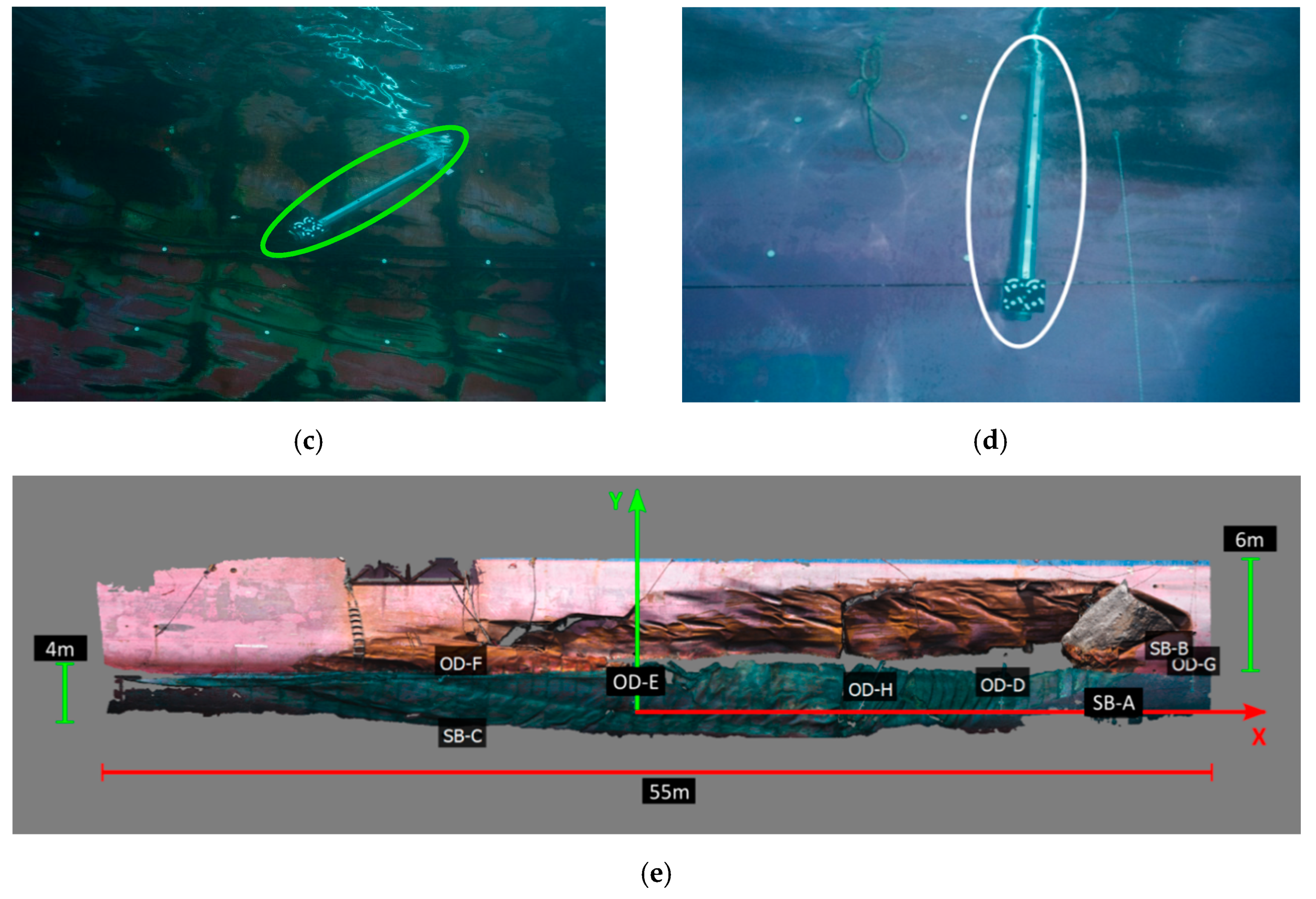
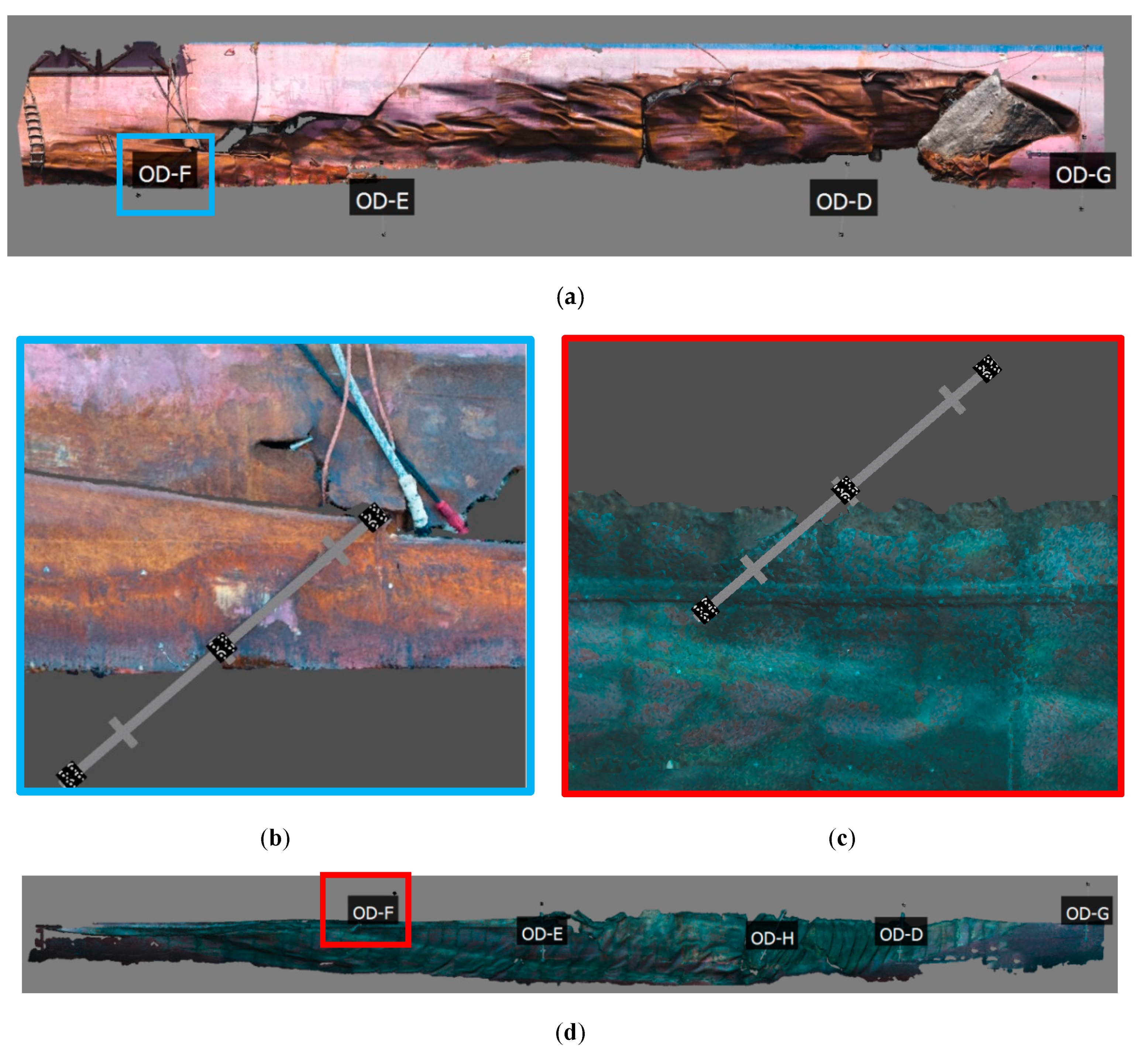
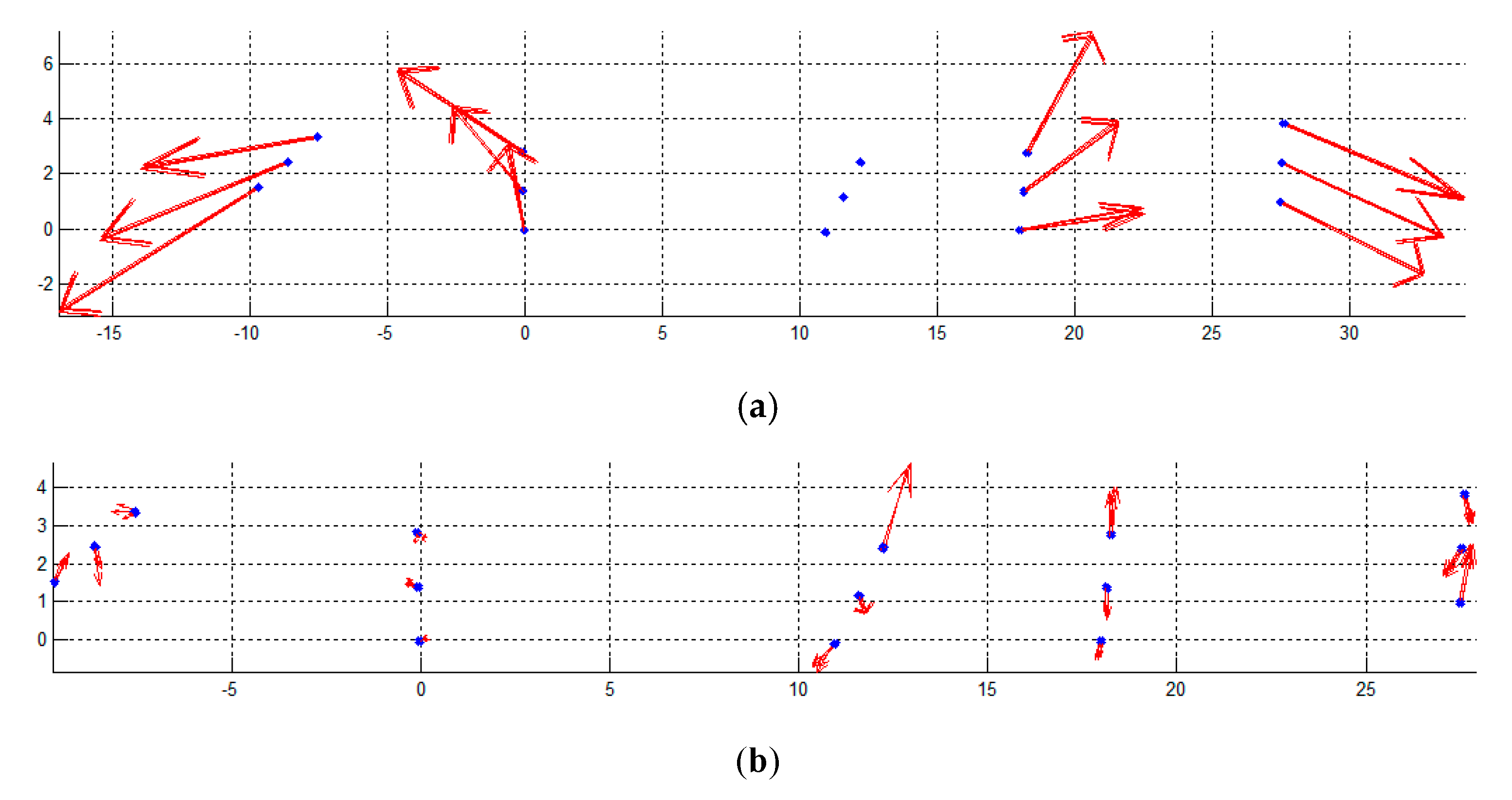
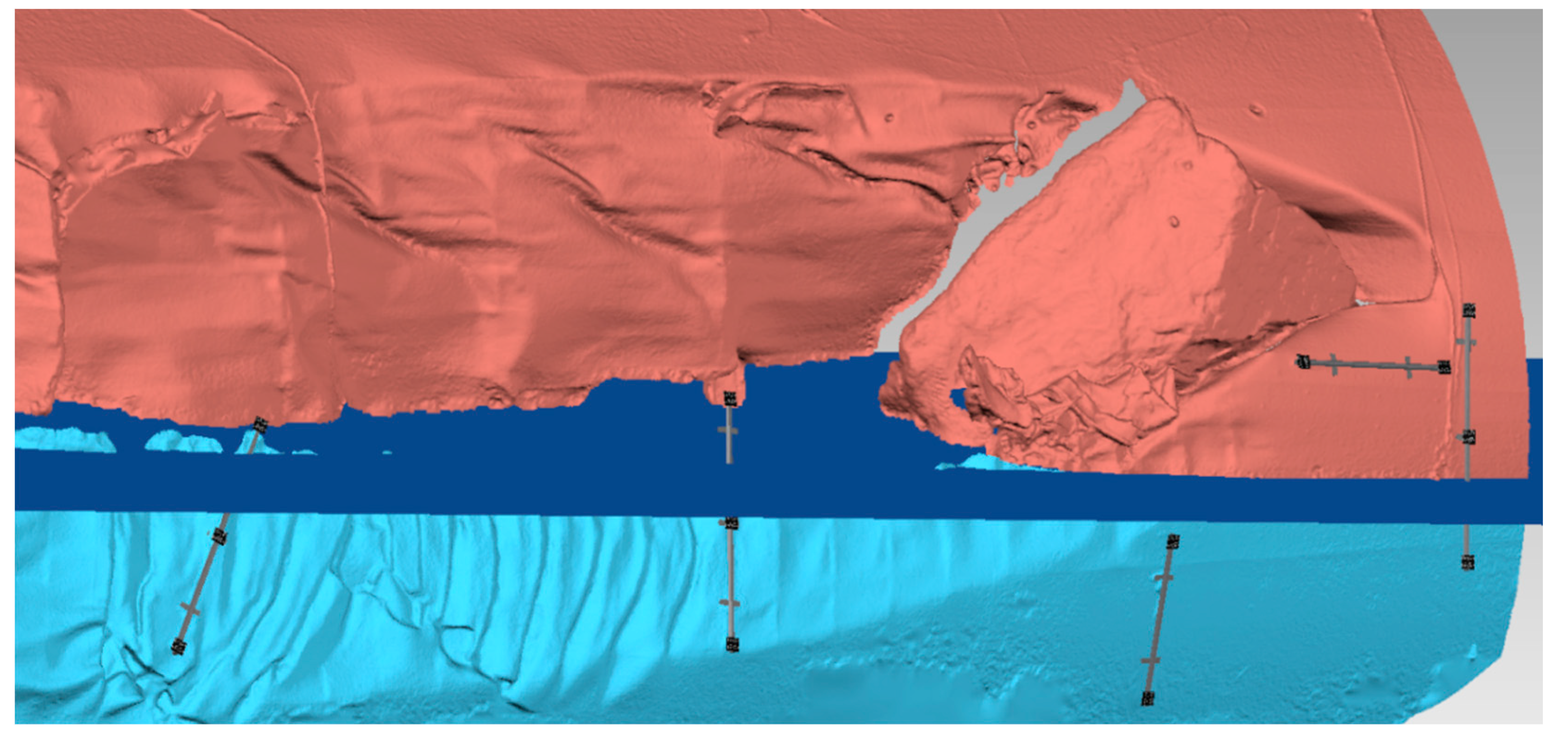
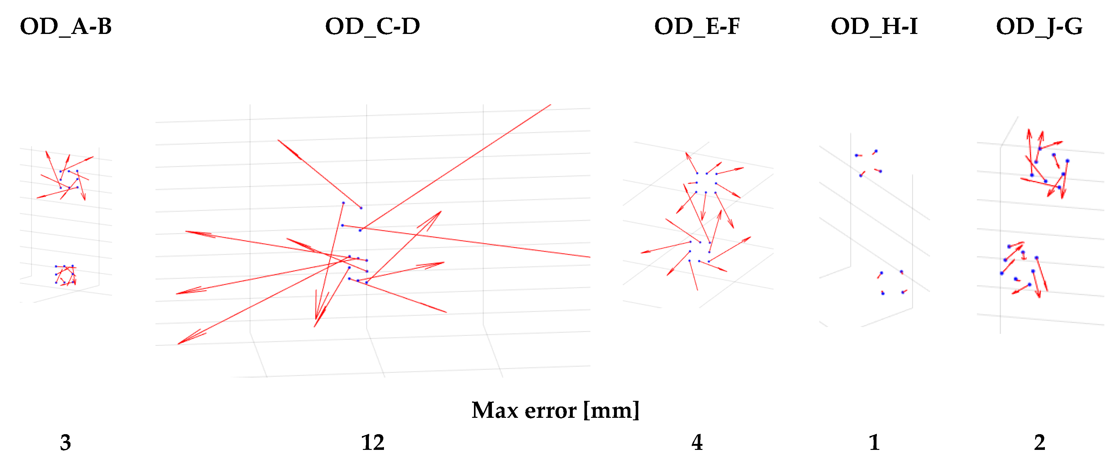
- Coarse alignment of two photogrammetric models: the first step of the coarse rigid transformation was carried out by mounting each single rod separately on the above and underwater photogrammetric models (Figure 12). Each transformation from the rod to both above and underwater independent models was computed without scale factor for preserving the higher accuracy scale of the rods. Two of the four targets of OD-H plate above the water were soiled by the fuel floating around the ship, making it not possible to compute the transformation to bring OD-H in the above-the-water photogrammetric model. After this step, the 3D coordinates of all the OD targets, except OD-H, were known in the both the photogrammetric models and were used to compute the similarity transformation for their assembling. Figure 13a shows the graphical results of the transformation, computed with 48 common points and without scale factor. Both the residual vectors, from the underwater reference system to the above the water reference system, and residual distribution are reported. The statistics are summarized in Table 4, which shows that the mean difference (in terms of root mean square error, RMSE) between the two models is of 0.016 m with a maximum of 0.027 m.
- Refinement of the alignment through independent model adjustment: the coordinates and transformation parameters computed in the previous step were used as approximations for the independent model free-network adjustment, where the scale factors of the rods were used as constraints. The results are shown in Figure 13b and Table 4. The spatial residuals from the comparison shown that, with respect to the coarse rigid transformation are reduced by a factor of about 10.
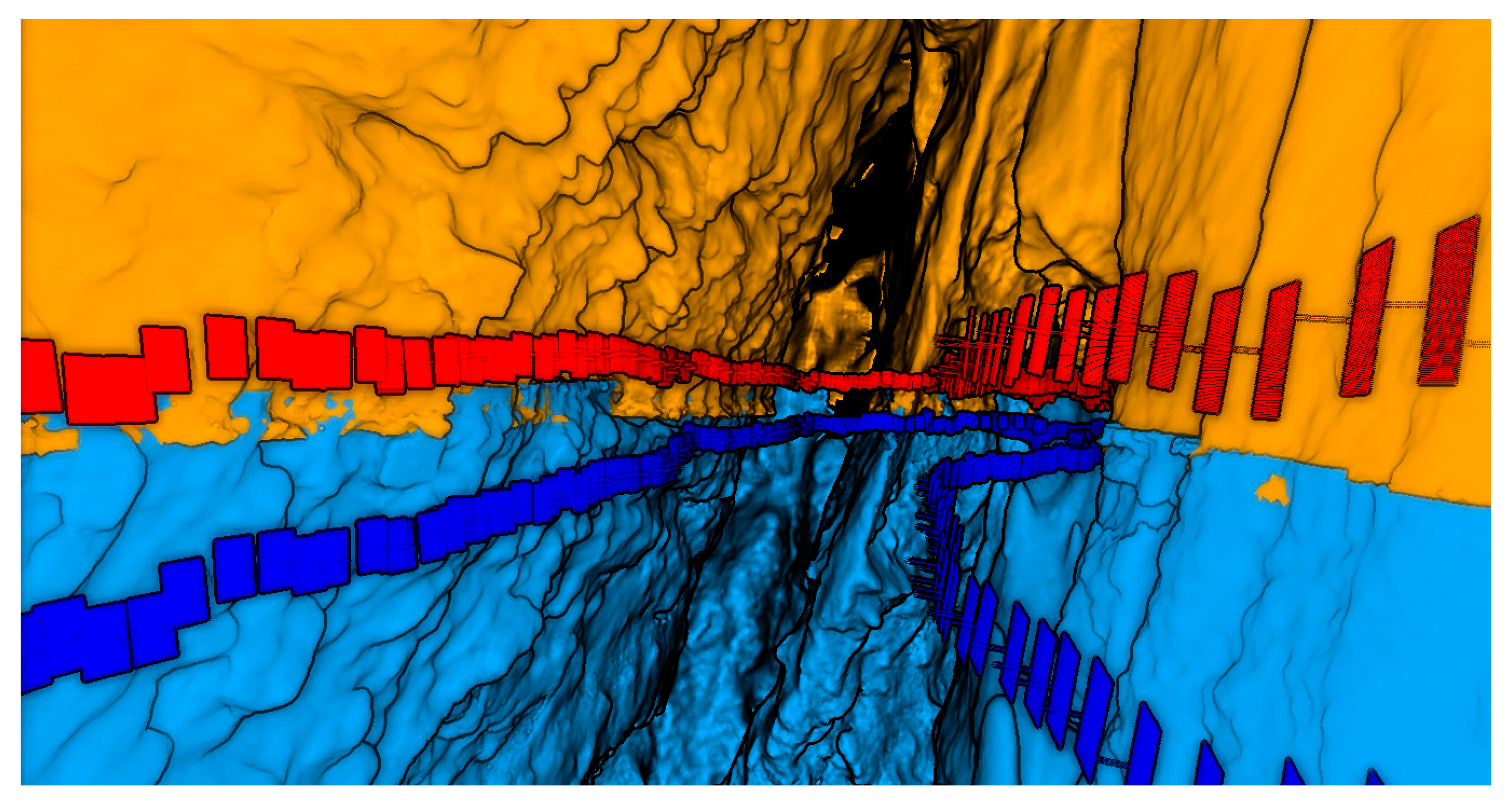
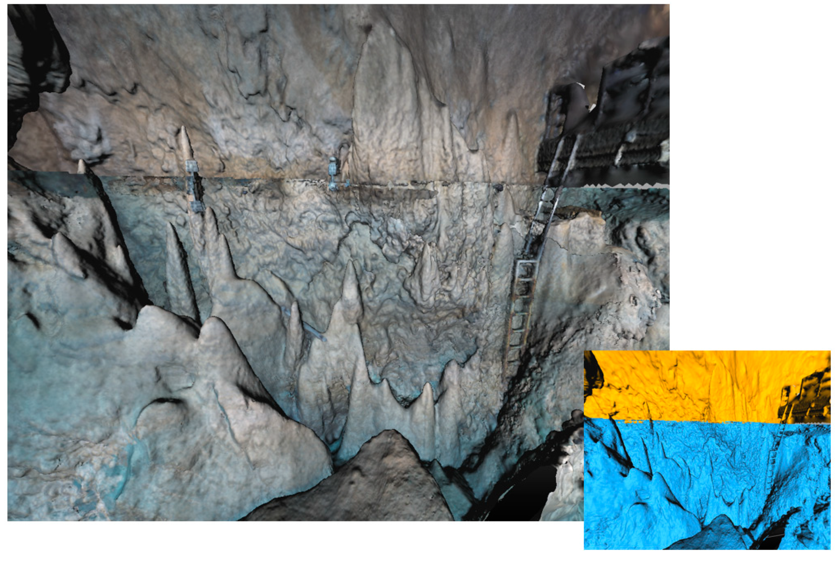
3.2. Case Study 2: Photogrammetric Survey of Semi-Submerged Environment Using a Synchronized Underwater Stereo-Camera Rig. The Case Study of Grotta Giusti
4. Discussions and Conclusions
Author Contributions
Funding
Acknowledgments
Conflicts of Interest
Appendix A
- is the vector of seven unknown transformation parameters
- are n functions of the unknowns, corresponding to Equation (1) for each 3D full point.
- is the vector of approximate observations obtained from the functional model computed with the approximate parameters .
- is the difference between measured and approximate observations, i.e., the vector of reduced observations.
Appendix B
- (i)
- Equations (A28) and (A29) are to be written for each observation (target coordinates on the rods) measured in each local coordinate system/independent model and
- (ii)
- Each target, being visible in two models (one rod and above or underwater), provides six observations.
- is the mean variance of object point coordinates.
- n is the number of points.
- is the cofactor of object point coordinates.
- are sub-blocks of the design matrix A containing the partial derivatives of the observation equations with respect to the transformation parameters from the local coordinate systems , , and to the final free-network datum . Each sub-block features a number of rows equal to the number of targets visible in the corresponding model and seven columns, i.e., the number of unknown transformation parameters.
- are sub-blocks of the design matrix A containing the partial derivatives of the observation equations with respect to the coordinates of points in the final coordinate system . Evidently, the sub-block related to one model will display zero elements in correspondence of those points that are not visible in it and the number of row will be equal to the number of measured targets.
- (i)
- The total number of rows of the design matrix will be equal to the sum of all the observations, i.e., targets visible in all the photogrammetric models plus the seven constraint equations for the free network solution. It corresponds to the length of the reduced observation vector plus the zero elements of constraint equations:
- (ii)
- The number of columns of the design matrix is equal to elements of the correction vector of the unknowns, i.e., the seven transformation parameters of all the systems and the target coordinates in the free network datum ground system :
References
- Floating Wind Turbine. Available online: https://en.wikipedia.org/wiki/Floating_wind_turbine (accessed on 15 January 2020).
- Berkas: Bridge over Øresund. Available online: https://id.wikipedia.org/wiki/Berkas:Bridge_over_%C3%98resund.jpg (accessed on 4 February 2020).
- Oil Platform in the North Sea. Available online: https://commons.wikimedia.org/wiki/File:Oil_platform_in_the_North_Sea.jpg (accessed on 4 February 2020).
- MV Princess of the Stars. Available online: https://en.wikipedia.org/wiki/MV_Princess_of_the_Stars (accessed on 15 January 2020).
- Switzerland-03436 Chapel Bridge. Available online: https://www.flickr.com/photos/archer10/23215035294/in/photostream/ (accessed on 15 January 2020).
- Grotte di Nettuno (1). Available online: https://www.flickr.com/photos/archer10/23215035294/in/photostream/ (accessed on 15 January 2020).
- Drap, P.; Merad, D.; Boï, J.M.; Boubguira, W.; Mahiddine, A.; Chemisky, B.; Seguin, E.; Alcala, F.; Bianchimani, O.; Environnement, S. October. ROV-3D, 3D Underwater Survey Combining Optical and Acoustic Sensor; VAST: Stoke-on-Trent, UK, 2011; pp. 177–184. [Google Scholar]
- Moisan, E.; Charbonnier, P.; Foucher, P.; Grussenmeyer, P.; Guillemin, S.; Koehl, M. Adjustment of Sonar and Laser Acquisition Data for Building the 3D Reference Model of a Canal Tunnel. Sensors 2015, 15, 31180–31204. [Google Scholar] [CrossRef] [PubMed] [Green Version]
- Van Der Lucht, J.; Bleier, M.; Leutert, F.; Schilling, K.; Nüchter, A. Structured-Light Based 3d Laser Scanning Of Semi-Submerged Structures. ISPRS Ann. Photogramm. Remote Sens. Spat. Inf. Sci. 2018, 4, 287–294. [Google Scholar] [CrossRef] [Green Version]
- Menna, F.; Nocerino, E.; Troisi, S.; Remondino, F. A photogrammetric approach to survey floating and semi-submerged objects. SPIE Optical. Metrol. 2013, 8791, 87910. [Google Scholar]
- Menna, F.; Nocerino, E.; Remondino, F. Photogrammetric modelling of submerged structures: Influence of underwater environment and lens ports on three-dimensional (3D) measurements. In Latest Developments in Reality-Based 3D Surveying and Modelling; MDPI: Basel, Switzerland, 2018; pp. 279–303. [Google Scholar]
- Nocerino, E.; Menna, F.; Farella, E.; Remondino, F. 3D Virtualization of an Underground Semi-Submerged Cave System. Int. Arch. Photogramm. Remote Sens. Spat. Inf. Sci. ISPRS Arch. 2019, 42, 857–864. [Google Scholar] [CrossRef] [Green Version]
- Kraus, K.; Waldhäusl, P. Photogrammetry. Fundamentals and Standard Processes; Dümmmler Verlag: Bonn, Germany, 1993; Volume 1. [Google Scholar]
- Faig, W. Aerotriangulation. Lecture Notes no. 40, Geodesy and Geomatics Engineering, UNB. 1976. Available online: http://www2.unb.ca/gge/Pubs/LN40.pdf (accessed on 11 February 2020).
- Shortis, M.; Harvey, E.; Abdo, D. A Review of Underwater Stereo-image Measurement for Marine Biology and Ecology Applications. Oceanogr. Mar. Biol. 2009, 2725, 257–292. [Google Scholar]
- Menna, F.; Nocerino, E.; Remondino, F.; Shortis, M. Investigation of a consumer-grade digital stereo camera. In Videometrics, Range Imaging, and Applications XII; and Automated Visual Inspection. Int. Soc. Opt. Photonics 2013, 8791, 879104. [Google Scholar]
- Lerma, J.L.; Navarro, S.; Cabrellesds, M.; Seguí, A.E. Camera Calibration with Baseline Distance Constraints. Photogramm. Rec. 2010, 25, 140–158. [Google Scholar] [CrossRef]
- Collision of Costa Concordia DSC4191. Available online: https://commons.wikimedia.org/wiki/File:Collision_of_Costa_Concordia_DSC4191.jpg (accessed on 4 February 2020).
- Costa Barrier. Available online: https://commons.wikimedia.org/wiki/File:Costa-barrier.svg (accessed on 4 February 2020).
- Nocerino, E.; Menna, F.; Remondino, F. Accuracy of typical photogrammetric networks in cultural heritage 3D modeling projects. ISPRS-Int. Arch. Photogramm. Remote. Sens. Spat. Inf. Sci. 2014, XL-5, 465–472. [Google Scholar] [CrossRef] [Green Version]
- James, M.R.; Robson, S. Mitigating systematic error in topographic models derived from UAV and ground-based image networks. Earth Surf. Process. Landf. 2014, 39, 1413–1420. [Google Scholar] [CrossRef] [Green Version]
- Nocerino, E.; Menna, F.; Remondino, F.; Saleri, R. Accuracy and block deformation analysis in automatic UAV and terrestrial photogrammetry-Lesson learnt. ISPRS Annals of the Photogrammetry, Remote Sensing and Spatial Information Sciences. In Proceedings of the 24th Internet CIPA Symposium, Strasbourg, France, 2–6 September 2013; pp. 203–208. [Google Scholar]
- Rupnik, E.; Nex, F.; Toschi, I.; Remondino, F. Aerial multi-camera systems: Accuracy and block triangulation issues. ISPRS J. Photogramm. Remote. Sens. 2015, 101, 233–246. [Google Scholar] [CrossRef]
- Agisoft. Available online: https://www.agisoft.com/ (accessed on 4 February 2020).
- Pix4D. Available online: https://www.pix4d.com/ (accessed on 4 February 2020).
- 3DF ZEPHYR. Available online: https://www.3dflow.net/3df-zephyr-pro-3d-models-from-photos/ (accessed on 4 February 2020).
- MicMac. Available online: https://micmac.ensg.eu/index.php/Accueil (accessed on 4 February 2020).
- EOS PhotoModeler. Available online: https://www.photomodeler.com/ (accessed on 4 February 2020).
- Photometrix Australis. Available online: https://www.photometrix.com.au/ (accessed on 4 February 2020).
- Forlani, G. Sperimentazione del nuovo programma CALGE dell’ITM. Bollettino SIFET. Boll. Della Soc. Ital. Topogr. Fotogramm. 1986, 2, 63–72. [Google Scholar]
- Orient. Available online: https://photo.geo.tuwien.ac.at/photo/software/orient-orpheus/introduction/orpheus/ (accessed on 4 February 2020).
- MATLAB. Available online: www.mathworks.com/products/matlab.html (accessed on 4 February 2020).
- CloudCompare. Available online: http://www.cloudcompare.org/ (accessed on 15 January 2020).
- Kazhdan, M.; Bolitho, M.; Hoppe, H. Poisson surface reconstruction. In Proceedings of the 4th Eurographics Symposium on Geometry Processing, Cagliari, Sardinia, 26–28 June 2006. [Google Scholar]
- Rodríguez-Gonzálvez, P.; Nocerino, E.; Menna, F.; Minto, S.; Remondino, F. 3D Surveying & Modeling of Underground Passages in WWI Fortifications. ISPRS-Int. Arch. Photogramm. Remote. Sens. Spat. Inf. Sci. 2015, 40, 17–24. [Google Scholar]
- Nocerino, E.; Menna, F.; Troisi, S. High accuracy low-cost videogrammetric system: An application to 6 DOF estimation of ship models. SPIE Opt. Metrol. 2013, 8791, 87910. [Google Scholar]
- Nocerino, E.; Nawaf, M.M.; Saccone, M.; Ellefi, M.B.; Pasquet, J.; Royer, J.-P.; Drap, P. Multi-camera system calibration of a low-cost remotely operated vehicle for underwater cave exploration. ISPRS-Int. Arch. Photogramm. Remote. Sens. Spat. Inf. Sci. 2018, 42, 329–337. [Google Scholar] [CrossRef] [Green Version]
- Menna, F.; Nocerino, E.; Fassi, F.; Remondino, F. Geometric and Optic Characterization of a Hemispherical Dome Port for Underwater Photogrammetry. Sensors 2016, 16, 48. [Google Scholar] [CrossRef] [PubMed] [Green Version]
- Brinker, R.C.; Minnick, R. (Eds.) The Surveying Handbook; Springer: Berlin/Heidelberg, Germany, 1995. [Google Scholar]
- Ghilani, C.D. Adjustment Computations: Spatial Data Analysis; John Wiley & Sons: Hoboken, NJ, USA, 2010. [Google Scholar]
- Mikhail, E.M.; Ackermann, F.E. Observations and Least Squares; IEP: New York, NY, USA, 1976. [Google Scholar]
- Mikhail, E.M.; Bethel, J.S.; McGlone, J.C. Introduction to Modern Photogrammetry; John Wiley & Sons Inc.: Hoboken, NJ, USA, 2001. [Google Scholar]
- Beinat, A.; Crosilla, F. Generalized Procrustes analysis for size and shape 3-D object reconstructions. In Optical 3-D Measurements Techniques V; Gruen, A., Kahmen, H., Eds.; Wichmann Verlag: Vienna, Austria, 2001; pp. 345–353. [Google Scholar]
- Faig, W. Aerial Triangulation and Digital Mapping: Lecture Notes for Workshops Given in 1984-85; School of Surveying, University of New South Wales: Sydney, Austria, 1986. [Google Scholar]
- Grafarend, E.W. Optimization of Geodetic Networks. Can. Surv. 1974, 28, 716–723. [Google Scholar] [CrossRef]
- Cooper, M.A.R.; Cross, P.A. Statistical concepts and their application in photogrammetry and surveying. Photogramm. Record 1988, 12, 637–663. [Google Scholar] [CrossRef]
- Dermanis, A. The photogrammetric inner constraints. ISPRS J. Photogramm. Remote. Sens. 1994, 49, 25–39. [Google Scholar] [CrossRef]
- Fraser, C.S. Network design considerations for non-topographic photogrammetry. Photogramm. Eng. Remote Sens. 1984, 50, 1115–1126. [Google Scholar]
| 1 | Also known as seven-parameter rigid transformation and corresponding to a 3D Helmert transformation. |
| 2 | seven transformation parameters are three translations, which represent the coordinates of the origin of one coordinate system with respect to the other, three rotation angles and one scale parameter, if an isotropic scale factor can be assumed for the three coordinate axes (rigid body assumption). In this case the transformation is also known as conformal or isogonal. |
| 3 | This rotation matrix is the transpose of (3). |
| 4 | Several SFM tools [24,25,26,27] for step 1 and photogrammetric software packages [28,29,30,31] for step 3 were tested. The results obtained from the different software packages were not significantly different, thus, Refs. [24] and [28] were selected for their flexibility and easier accessibility and integration in an own-developed procedure written in [32]. Step 2 and the alignment procedure were implemented in [32] by the authors. Step 4 was performed in [24] and the meshing in [33]. |
| 5 |


| Original Tie Points | Filtered Tie Points | Percentage Reduction | |
|---|---|---|---|
| Above the Water | |||
| Number of three-dimensional (3D) Point | 151,824 | 5689 | 96% |
| Number of Image Observations | 940,636 | 56,473 | 94% |
| Average Number of Tie Points Per Image | 282 | ||
| Underwater | |||
| Number of 3D Point | 420,328 | 11,313 | 97% |
| Number of Image Observations | 1070,626 | 53,263 | 95% |
| Average Number of Tie Points Per Image | 67 | ||
| Number of Intersecting Optical Rays | Number of Strips | Intersection Angle | |
|---|---|---|---|
| Above the water | |||
| Mean | 10 | 2 | 41° |
| Standard deviation | 7 | 1 | 19° |
| Max | 32 | 4 | 90° |
| Underwater | |||
| Mean | 5 | 2 | 28° |
| Standard deviation | 4 | 1 | 15° |
| Max | 38 | 4 | 89° |
| Above-the-Water | Underwater | |||
|---|---|---|---|---|
| Object Space | sXYZ Precision vector length [m] | Mean | 0.0026 | 0.0027 |
| Stdv | 0.0008 | 0.0010 | ||
| Max | 0.0051 | 0.0060 | ||
| Image Space | Root mean square reprojection Error [Pixel] | Mean | 0.336 | 0.449 |
| Stdv | 0.137 | 0.134 | ||
| Max | 0.826 | 1.129 | ||
| Max residual error [Pixel] | Mean | 0.523 | 0.741 | |
| Stdv | 0.226 | 0.234 | ||
| Max | 1.287 | 1.683 | ||
| RMSE X [m] | RMSE Y [m] | RMSE Z [m] | RMSE Length [m] | RMSE Mean (Magnitude) [m] | Max Residual [m] |
|---|---|---|---|---|---|
| Coarse Alignment | |||||
| 0.0051 | 0.003 | 0.0164 | 0.0174 | 0.0159 | 0.0269 |
| Independent Models Adjustment | |||||
| 0.003 | 0.0008 | 0.0011 | 0.0014 | 0.0011 | 0.0037 |
© 2020 by the authors. Licensee MDPI, Basel, Switzerland. This article is an open access article distributed under the terms and conditions of the Creative Commons Attribution (CC BY) license (http://creativecommons.org/licenses/by/4.0/).
Share and Cite
Nocerino, E.; Menna, F. Photogrammetry: Linking the World across the Water Surface. J. Mar. Sci. Eng. 2020, 8, 128. https://doi.org/10.3390/jmse8020128
Nocerino E, Menna F. Photogrammetry: Linking the World across the Water Surface. Journal of Marine Science and Engineering. 2020; 8(2):128. https://doi.org/10.3390/jmse8020128
Chicago/Turabian StyleNocerino, Erica, and Fabio Menna. 2020. "Photogrammetry: Linking the World across the Water Surface" Journal of Marine Science and Engineering 8, no. 2: 128. https://doi.org/10.3390/jmse8020128