The Contribution of Multispectral Satellite Image to Shallow Water Bathymetry Mapping on the Coast of Misano Adriatico, Italy

Abstract

The results of absolute satellite-derived bathymetry (SDB) are presented in the current study. A comparative analysis was conducted on empirical methods in order to explore the potential of SDB in shallow water on the coast of Misano, Italy. Operations were carried out by relying on limited in situ water depth data to extract and calibrate bathymetry from a QuickBird satellite image acquired on a highly dynamic coastal environment. The image was processed using the log-band ratio and optimal band ratio analysis (OBRA) methods. Preprocessing steps included the conversion of the raw satellite image into top of atmosphere reflectance, spatial filtering, land and water classification, the determination of the optimal OBRA spectral band pairs, and the estimation of relative SDB. Furthermore, calibration and vertical referencing were performed via in situ bathymetry acquired in November 2007. The relative bathymetry obtained from different band ratios were vertically referenced to the local datum using in situ water depth in order to obtain absolute SDB. The coefficient of determination (R²) and vertical root mean square error (RMSE) were computed for each method. A strong correlation with in situ field bathymetry was observed for both methods, with R² = 0.8682 and RMSE = 0.518 m for the log-band ratio method and R² = 0.8927–0.9108 and RMSE = 0.35 m for the OBRA method. This indicated a high degree of confidence of the SDB results obtained for the study area, with a high performance of the OBRA method for SDB mapping in turbid water.

1. Introduction

Coastal zones are one of the most dynamic and rapidly changing environments at the global scale. Such changes are strongly induced by anthropogenic pressure in synergy with natural coastal processes and changes in global climate [1]. In fact, coastal areas are amongst the most heavily populated areas in the world, with the presence of intensive economic development. At present, approximately 44% of the global human population lives within 150 km of the coastal zone [2,3]. Population growth and economic pressure in coastal zones will continue to increase, not only in the near future, but also centuries from now [4]. Therefore, considering the projected global climate change, it is crucial to comprehend the evolution of the coastal zone. For this reason, coastal zone monitoring is an essential process for sustainable coastal management and environmental protection [5]. The continuous environmental monitoring of coastal areas is required for the maintenance of coastal environments and to estimate the sustainability of current practice [6]. The processes, whether natural or artificial, promote sand transportation (erosion, transportation, and sediment deposition) and alter seabed morphology, both of which have important roles in the dynamic behavior of coastal areas [7]. Consequently, the monitoring of offshore zones is also required for the analysis and projection of coastal dynamics and environmental change [6,8]. Bathymetry is one of the key factors used by scientists, hydrographers, and decision-makers operating in coastal zones. It provides useful information on ecological and geomorphological process occurring in coastal areas. Accurate and reliable bathymetry information is important for coastal erosion studies, maritime navigation, the mapping and monitoring of benthic habits, dredging planning, and coastal management in general. Traditional methods for bathymetry surveys use boats and ships equipped with multi-beam echo sounder or single beam echo sounder [9,10] or topo-bathymetry Lidar [11,12]. Such methods are able provide accurate water depth information; however, they are expensive and inefficient in hard-to-reach shallow waters [13]. Multispectral satellite images present an alternative solution for research on shallow water bathymetry. With their large swath width, satellites are able to provide information over a large geographic area at a very low cost [14]. In particular, multispectral satellite images are able to provide bathymetry information in shallow waters [15], aiding in the improvement of the monitoring of shoreline variability [16]. In addition, studies conducted using stereo images [17,18,19] have demonstrated a great potential for shallow water bathymetry mapping using data from remote sensing.

Jawak et al. [20] discussed bathymetry mapping technologies using satellite remote sensing. They highlighted two types of satellite sensors capable of providing water depth information: (1) active satellite sensors or altimeters, which emit artificial radiation to study the Earth’s surface or atmospheric features (e.g., the synthetic aperture radar—SAR), and (2) passive satellite sensors, which detect solar radiation reflected from the Earth (e.g., multispectral or optical satellite sensors). Passive sensors have been used in satellite-derived bathymetry (SDB) studies via the estimation of the water depth on the basis of the digital numbers (DN) of each pixel (representing reflectance or backscatter) of an image acquired in the visible and/or near infrared (NIR) and microwave parties of the electromagnetic spectrum [20].

The advancement of SDB has revolutionized the acquisition of water depth information with the use of remote sensing techniques to obtain information about coastal environments [21]. Since their establishment four decades ago [22] with the launch of Landsat-1 on 23 July 1972, many methods have been developed for SDB. These methods can be grouped into empirical, semi-analytic, and physical-based approaches [23]. They rely on wavelength of light and its propagation angle in the air and in water, with the only difference being in the number of parameters and in situ data involved in the processing of satellite images. Further details of these approaches can be found in [24], with a short summary provided by [25,26]. Bathymetry from Earth observation data has been explored by many authors [27,28,29,30,31,32,33,34,35] under various domains, such as underwater archaeology [25] and natural disaster evaluation [34]. The authors of [36] used a simplified radiative transfer equation to retrieve both SDB and water column in shallow waters without the need for a formal atmospheric correction technique (i.e., the conversion of relative radiance into calibrated reflectance) or the use of existing depth sounding data. However, they noted that some sensor configurations (e.g., near-nadir view angle) and environmental conditions—including a clear sky, the time the sun is highest in the sky, and less suspended water particles (clear water)—must be respected in order to obtain a good quality satellite image with less atmospheric and glint effects for SDB study.

Bathymetry studies conducted in highly turbid water generally apply the radiative transfer equation on multispectral images [37], or perform radiative transfer simulations on hyperspectral images [38]. However the presence of turbidity reduces the visibility and impacts the light propagation through the water, whereas the light sensed at the top-of-atmosphere (TOA) is strongly influenced by atmospheric composition [39]. Thus, by taking into account the changes in multispectral images caused by atmospheric corrections over very bright and dark coastal waters [40], the main objective of the current study was to harness the small amount of water depth information present in the blue, green, red, and NIR spectral bands of TOA reflectance acquired over turbid water. More specifically, we conducted a quantitative comparative analysis of the empirical methods commonly used in bathymetric studies, namely, the log-band ratio and optimal band ratio analysis (OBRA) methods. We intended to explore the potential of these two methods for a multispectral satellite image acquired over a coastal area in order to determine which spectral band ratio was able to provide high accurate water depth information in highly dynamic waters.

Although the scale and the accuracy of the absolute SDB obtained using these two methods relies on suitable in-situ bathymetric datasets [41] and the number of points [42] used to calibrate and validate relative SDB, in this study, we presented a calibration/validation methodology that required a limited number of sounding points. The methodology was based on the equations of Stumpf et al. [28] and Legleiter et al. [43]. These empirical methods are based on the theory that light is attenuated exponentially with bathymetry and that the impacts of seafloor reflectance are minimized at different spectral bands [20]. The log-band ratio, an enhanced version of the model described in [34], makes use of the blue and green bands to estimate relative SDB and in situ data for vertical referencing, whereas the NIR band is used for the separation of water and land. Furthermore, we used bathymetric field data acquired in November 2007 using a single-beam echo sounder. This method reduces the impact of atmospheric conditions, the water column, and the seafloor on the propagation of light via the use of electromagnetic bands affected simultaneously by these factors [44]. Furthermore, the OBRA method is a robust and optimized band ratio method for SDB estimations that explores all available pair bands to identify the pair that is less sensitive to substrate variability and exhibits the closest linear relationship with available in situ water depth information [45].

This methodology contributes to the use of satellite images in shallow water bathymetry studies by allowing the integration of available bathymetry field data and the use of multispectral data to calibrate and enhance the accuracy of relative shallow water bathymetry. To extract information regarding water depth on high resolution satellite images, a series of pre-processing steps are required in order to convert raw QuickBird image (digital numbers) acquired in September 2007 into TOA reflectance. During the processing of the data, we followed a number of steps involving the removal of speckle noise, the separation of dry sand and water, the calculation of optical depth limit and relative bathymetry, and finally, statistical analysis and vertical referencing to local datum to obtain absolute SDB.

2. Materials and Methods

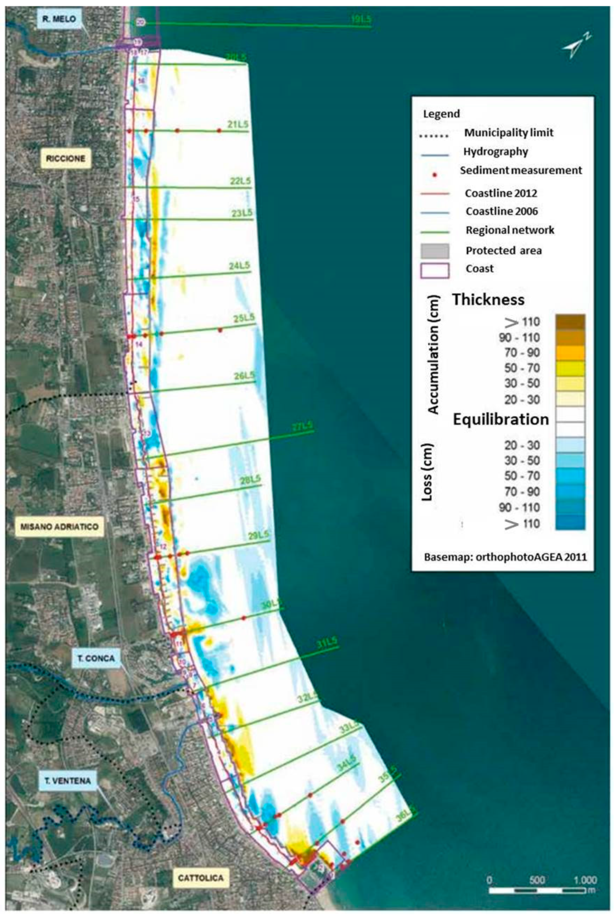
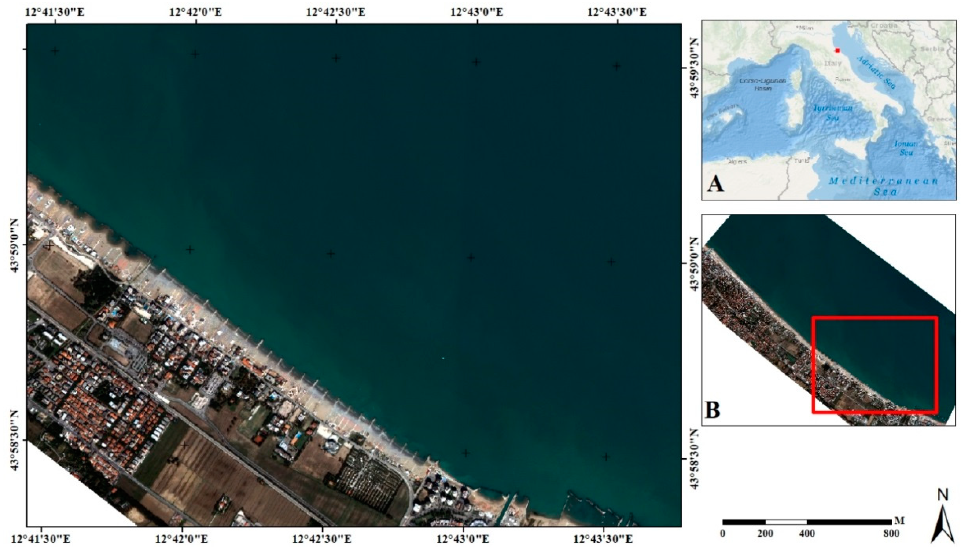
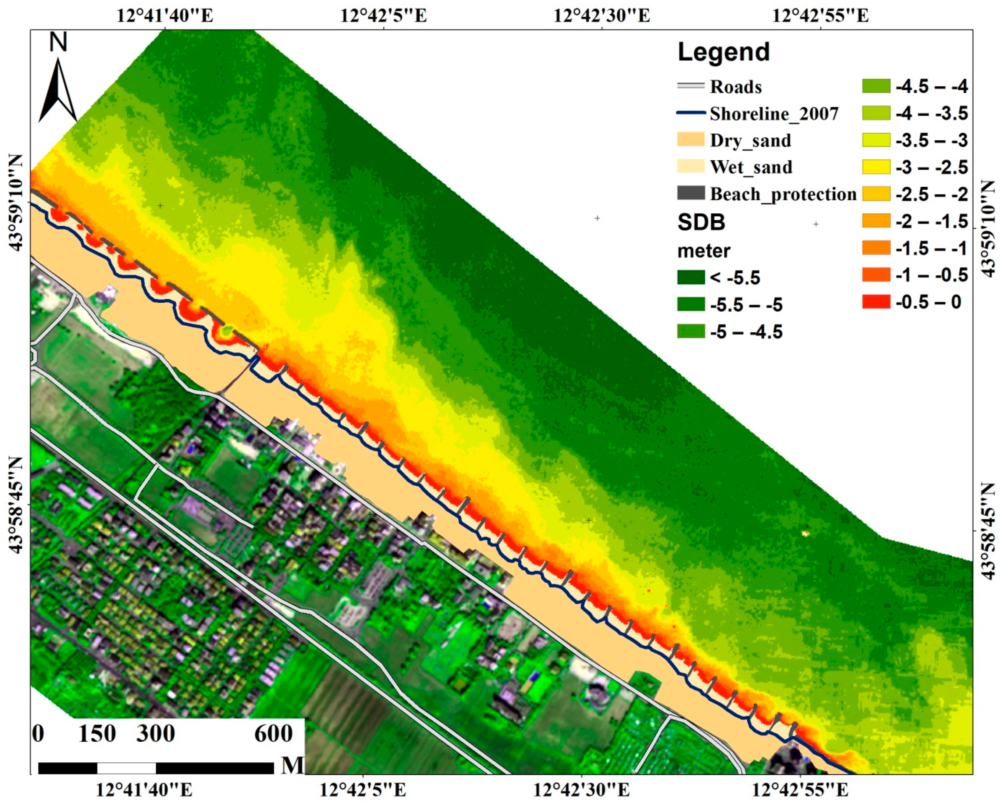
2.1. Area of Study

The coast of the Emilia-Romagna region is composed of sandy beaches stretching over 130 km and facing the northern Adriatic Sea in the northeast of Italy. It has undergone profound changes due to human activities, particularly since the beginning of the 20th century, and in particular due to the reclamation of large valleys, the leveling of extensive tracts of coastal dunes, and intense urbanization of backshore areas. These changes, combined with the natural decrease of sediment supply by rivers, climatic change, and subsidence, have caused significant beach erosion, which still persists despite many coastal defense interventions having been carried out between 1960 and 1980 [46,47]. Hard shore protection structures are widely distributed and protect over 60% of the regional coastline. Recently, the shorelines of protected areas have remained relatively stable due to human intervention, including widespread beach replenishment [48]. Misano Adriatico is a well-developed tourist resort in the Emilia-Romagna region close to Rimini and Riccione and located on the Northwest Adriatic Sea. Misano Adriatico beach is under erosion and is already artificially defended through hard structures and beach nourishment.

The Figure 1 depicts the accumulations and loss of sediments on the cost of Misano for the period of 2006–2012. Figure 1 was generated by comparing the results of multiple topo-bathymetric surveys conducted on the coast of Emilia-Romagna. More specifically, aerial photographs and a ground-based differential global positioning system (DGPS) were used for the monitoring of the shoreline evolution, whereas for bathymetric and topographic mapping, multibeam/single beam echosounders and dynamic laser-scanners were used, respectively. At the beginning of each survey, the bathymetric system was calibrated according to IHO S-44 specifications in order to guarantee high quality bathymetry data. In addition, a ground base station with a radio-modem was set up for the differential correction of the DGPS real-time kinematic (RTK) positioning system for all offshore and onshore survey activities. Detailed topographic maps of the emerged beaches were obtained via a dynamic laser scanner system installed on a vehicle, acquiring 1000 points per second along a path parallel to and 100–200 m away from the shoreline. The survey was conducted during low tide (−0.40 m) and calm sea conditions. Each topo-bathymetry survey conducted during 2006–2012 produced a digital terrain model (DTM) that was highly representative of the morphology of the emerged and submerged beaches, with a depth of up to 6–8 m. The map derived from the difference between the DTMs represents the change in altitude of the emerged and submerged beaches between 2006 and 2012 (Figure 1).

Nourishment has been carried out multiple times, using lime, gravel, and sand [50]. These materials dominate the sea bottom and complicate SDB study due to the presence and migration of suspended sediments in the sea. Moreover, the river run-off brings in substantial quantities of sediments that reduce the visibility and quality of sea water. High precision topo-bathymetry studies realized between 2000–2005 and 2006–2012 revealed changes in sand volumes followed by the movement of the ground [49,50]. Due to the availability of field data, we conducted a SDB along the coastline for 4 km from Malindi Biky Beach, in the south, to beach of Riccione area 3, in the north (Figure 2).

2.2. Dataset

We used a DigitalGlobe QuickBird satellite image obtained from European Space Imaging [51]. This image was acquired on 7 September 2007 at 10:24:06 UTC. The image had a spatial resolution of 2.4 m for multi-spectral sensors and 0.6 m for panchromatic band (

Table 1. Main characteristics of QuickBird image used in this study.

QuickBird Bands	Spatial Resolution	Radiometric Resolution	Absolute Radiometric Calibration Factors (W × m−2 × sr−1 × DN−1) and Effective Band Width (μm)
Panchromatic	0.6 m	450–900 nm	0.06447600 and 0.398
Blue	2.4 m	450–520 nm	0.01604120 and 0.068
Green	2.4 m	520–600 nm	0.01438470 and 0.099
Red	2.4 m	630–690 nm	0.01267350 and 0.071
Near infrared	2.4 m	760–900 nm	0.01542420 and 0.114

). Agreeable atmospheric conditions were present during the acquisition of the image, with 0% cloud cover, mean solar azimuth angle of 162.7°, mean off nadir view angle of 8°, and mean sun elevation of 51.2°.

Bathymetric surveys on the coast of Misano Adriatico started over two decades ago with yearly data acquisitions. The field data used for vertical referencing were provided by local authorities and were acquired during a bathymetry survey conducted in November 2017. In particular, Planimetry data were acquired using a topographic station on the ground with horizontal precision of 10 cm for subsidence correction and georeferencing. Bathymetric data were acquired using a boat equipped with sub-metric horizontal precision (Global Positioning System: GPS) and a 1 cm vertical precision single-beam echosounder. The survey data were ultimetrely projected to mean sea level using tide measures provided by a local tide station. The DraWinG output file formats contained water depth ranging from 0.5 to 6 m.

The total vertical uncertainty (TVU) along with total horizontal uncertainty are International Hydrographic Organization (IHO) reference standards used for quality and uncertainty assessment for hydrographic survey order. The TVU was used for evaluation of water depth vertical accuracy of in-situ data, and was estimated using Equation (1), whereas the maximum allowable horizontal uncertainty of in-situ data, at a 95% confidence level, was taken as 2 m. This in situ bathymetry data met required uncertainties of IHO standards for special order hydrographic surveys where a and b in Equation (1) are equal to 0.25 m and 0.0075, respectively [52].

$$TVU=\pm \sqrt{a^2+{\left(b\times z\right)}^2}$$

(1)

where a represents the uncertainty component that does not vary with depth, b is a coefficient representing the uncertainty component that varies with depth, z is the depth, and b × z represents the uncertainty component that varies with depth.

Persistent coastal erosion on Misano Adriatico and sediments used for beach nourishment change the optical properties of seawater. Although there were no available turbidity data in this region, the fine sediments used during beach nourishment [49] can increase suspended sediment concentration and ultimately increase the turbidity. This phenomenon can be observed from the satellite image, with high reflectance in the NIR band and a notable low reflectance in blue and green bands [53].

2.3. Software Used

ArcMap (v. 10.2.2, ESRI) and its geo-processing tools in ArcToolbox were used to conduct the pre-processing and processing of the data. In particular, ArcMap allows for the integration of the mathematical equations necessary for converting digital numbers (raw data) into TOA reflectance and for the processing of bathymetry information. Statistical analysis was performed using Microsoft Excel (v. 2010, Microsoft Corporation).

2.4. Pre-Processing of Data

The image obtained from European Space Imaging is OrthoReady (2A) imagery projected, based on ellipsoid WSG 84 UTM zone 33N, to the constant base elevation of Misano Adriatico coastal area. It is a radiometrically and sensor-corrected product with 23 m horizontal accuracy.

2.4.1. Radiometric Calibration and Correction

There are two steps involved in the transformation of radiometric data to TOA spectral radiance [54]. First, the QuickBird radiometrically corrected image pixel values (digital numbers) were converted to TOA band-integrated radiance pixels using the absolute radiometric calibration factor provided for each band in the IMD files of data product (Table 1), as described in Equation (2).

$$Lpixel,Band=absCalFactorband\ast Qpixel,Band$$

(2)

where$Lpixel,Band$ are TOA band-integrated radiance image pixels expressed in (W × m⁻² × sr⁻¹), $absCalFactorband$ is the absolute radiometric calibration factor expressed in (W × m⁻² × sr⁻¹ × DN⁻¹), and $Qpixel,Band$are radiometrically corrected image pixels expressed in (DN).

The second step is the transformation of TOA radiance image pixels, integrated for each band to TOA spectral radiance, by applying Equation (3) integrating the effective bandwidth (Δλ) provided for each band in the IMD files of data product (Table 1).

$$L\lambda Pixel,Band=\frac{\left(LPixel,Band\right)}{\left[∆\lambda Band\right]}(\mathrm{W}\times {\mathrm{m}}^{-2}\times {\mathrm{sr}}^{-2}\times \mathsf{\mu }{\mathrm{m}}^{-2})$$

(3)

where $L\lambda Pixel,Band$. are TOA spectral radiance image pixels averaged for each band, LPixel,Band are TOA radiance image pixels integrated for each band, and ΔλBand is the effective bandwidth for each band.

2.4.2. Transformation to TOA Spectral Reflectance Image Pixels

The TOA spectral radiance is the quantity of radiance that is saved by the sensor, expressed in watts per unit of source area, per unit of spectral response and per unit of wavelength (W × m⁻² × sr⁻¹ × μm⁻¹). This radiance is the amount of source energy on the surface, but also the amount of energy backscattered into the atmosphere, and can affect bathymetry studies. Thus, the absorbed and backscattered energy in the atmosphere should be removed from TOA reflectance. Equation (4) is used to convert TOA spectral radiance to TOA spectral reflectance.

$$\rho p=\frac{\pi \times L\lambda \times d2}{ESUN\lambda \times cos\left(\theta s\right)}$$

(4)

where $\rho p$ is the TOA reflectance, ESUNλ is the mean solar extra-atmospheric irradiance W × m⁻² × μm⁻¹, d is Earth–Sun distance obtained from Julian Day acquisition time and θs is the solar zenith angle equal to 90 degrees minus the sun elevation angle at the time of image acquisition, which was found in the IMD files provided with raw data.

Equations (1)–(4) were calculated using the spatial analyst tools/map algebra/raster calculator of the ArcToolbox window.

2.5. Data Processing and Bathymetry Extraction

Following [55], the QuickBird satellite image was processed in ArcMap 10.2.2 in order to extract SDB multispectral information.

2.5.1. SDB Retrieval

The pre-processing steps were performed in order to avoid the effect of atmosphere on the reflectance received by satellite sensors.

Water-leaving TOA reflectance is a function of the bottom reflectance, water depth, and the up-welling and down-welling operational diffuse attenuation coefficient. As the water depth increases, the bottom reflectance detected by the optic multispectral sensors decreases until it can no longer be detected [34]. With the use of empirical methods (e.g., linear-band log-band ratio and OBRA methods), shallow water bathymetry can be determined by analyzing water-leaving reflectance. The retrieval of SDB using empirical methods is based on the vertical referencing of the bathymetric model (relative SDB) on the local datum. This bathymetric model is obtained through the logarithmic transformations of spectral water-leaving reflectance. In situ bathymetric data is generally the main source of information used to determine the calibration parameters via linear regressions, which are then used for the fitting of the bathymetric model.

Log-Band Ratio Method

The ability of satellite sensors to collect water information in multispectral bands allows for research on seabed morphology and shallow bathymetry. For example, a methodological bathymetry approach using two spectral bands (blue, green) in conjunction with in situ bathymetry, taking into account the quality of water and the propagation of light through the water column [28], has been published.

Although most near infrared light is absorbed by clear water, it is still a useful parameter for the land/water boundary extraction process [56]. Green and blue light penetrate the water column and are exponentially attenuated as the water depth increases, leading to the principle of shallow water bathymetry extraction [40]. The log-band ratio method of Stumpf et al. [28] for SDB mapping assumes that the area has a uniform bottom and a log-band ratio of water-leaving reflectance that decreases linearly with water depth. In the current study, we assumed that water-leaving reflectance contributed to TOA reflectance, and applied Equation (5) for the estimation of SDB.

$$Z=m1\times \frac{ln\left(nRw\left(\lambda i\right)\right)}{ln\left(nRw\left(\lambda j\right)\right)}-m0$$

(5)

where Z(m) is absolute water depth (SDB), m1 is a tunable constant used to scale the ratio to the depth (gradient of the line or gain), Rw (dimensionless) is observed spectral reflectance, for the n-factor we can use any positive number large enough that for all the pixels in the image both the logarithms used in the ratio are positive, m0 is the offset for the depth of 0 m (z = 0, y-axis intercept), λi is the blue band, and λj is the green band.

OBRA Method

The log-band ratio method has the advantage of being less sensitive to substrate variation types. This has been demonstrated by Stumpf et al. [28], who found that the spectral band reflectance ratios of different benthic cover types at the same water depth have approximately equal values. The availability of multispectral satellite images containing different water information, such as water depth, suspended particles, seabed vegetation, and seafloor biomass, enhances the possibility of band ratio variations. In order to reduce the impact of bottom types, it is important to carefully choose pair bands for more efficient relative SDB estimations. The OBRA method of Legleiter et al. [43] uses optimal spectral band pairs for a range of water depths and substrate types. It identifies spectral band pairs that are minimally affected by bottom type variabilities; more specifically, two spectral bands with a high coefficient of determination (R²) with the relative SDB estimated by Equation (6) and in-situ bathymetry data among all possible band ratios. The bathymetric information is subsequently determined by applying Equation (7).

$$rSDB=\frac{ln\left(nRw\left(\lambda i\right)\right)}{ln\left(nRw\left(\lambda j\right)\right),}$$

(6)

$$Z=m1\times rSDB-m0$$

(7)

where λi is spectral band i, λj is spectral band j, and rSDB is the relative satellite-derived bathymetry obtained from a pair of spectral bands.

2.5.2. Application of SDB Algorithm and Vertical Referencing

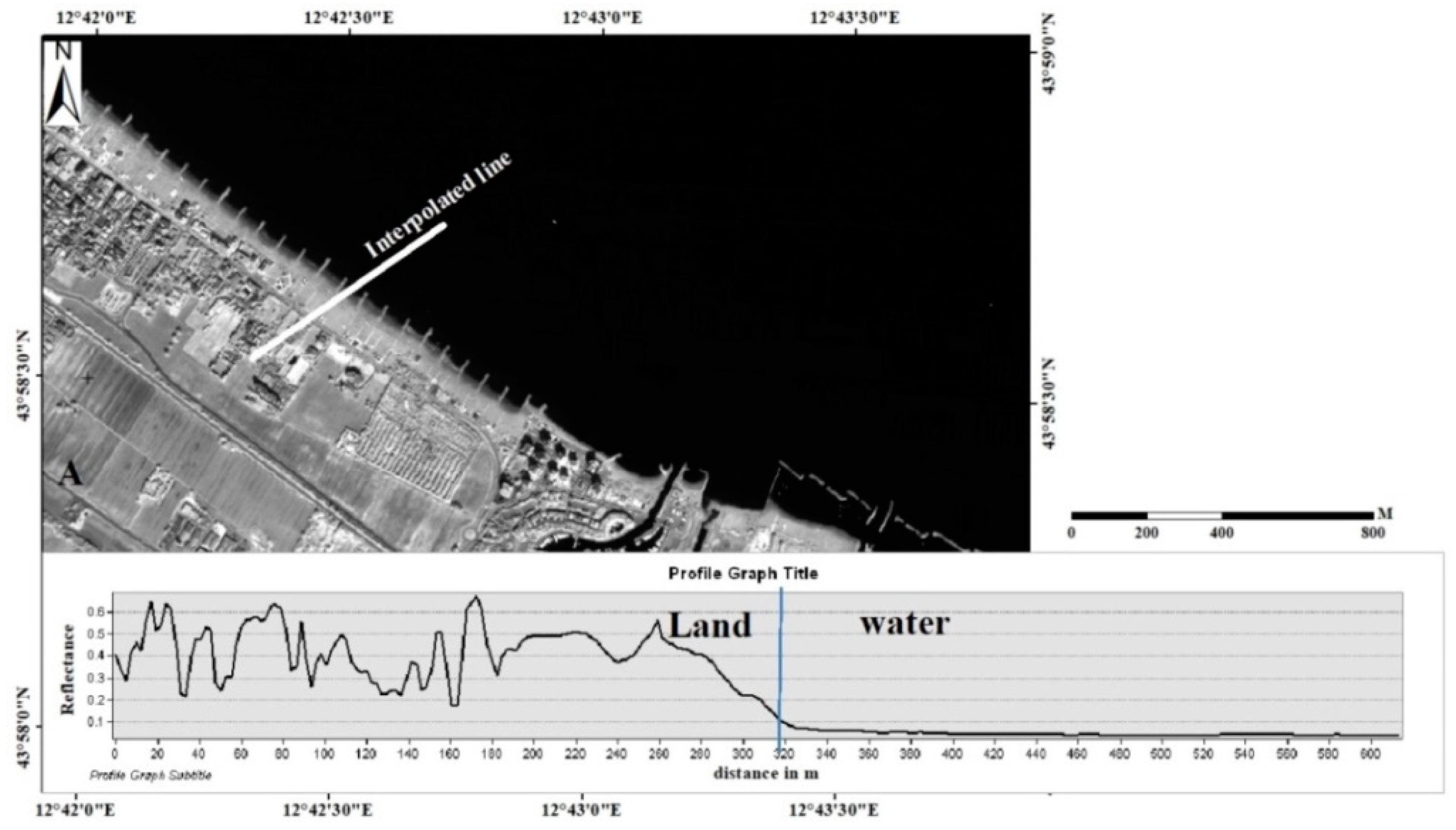
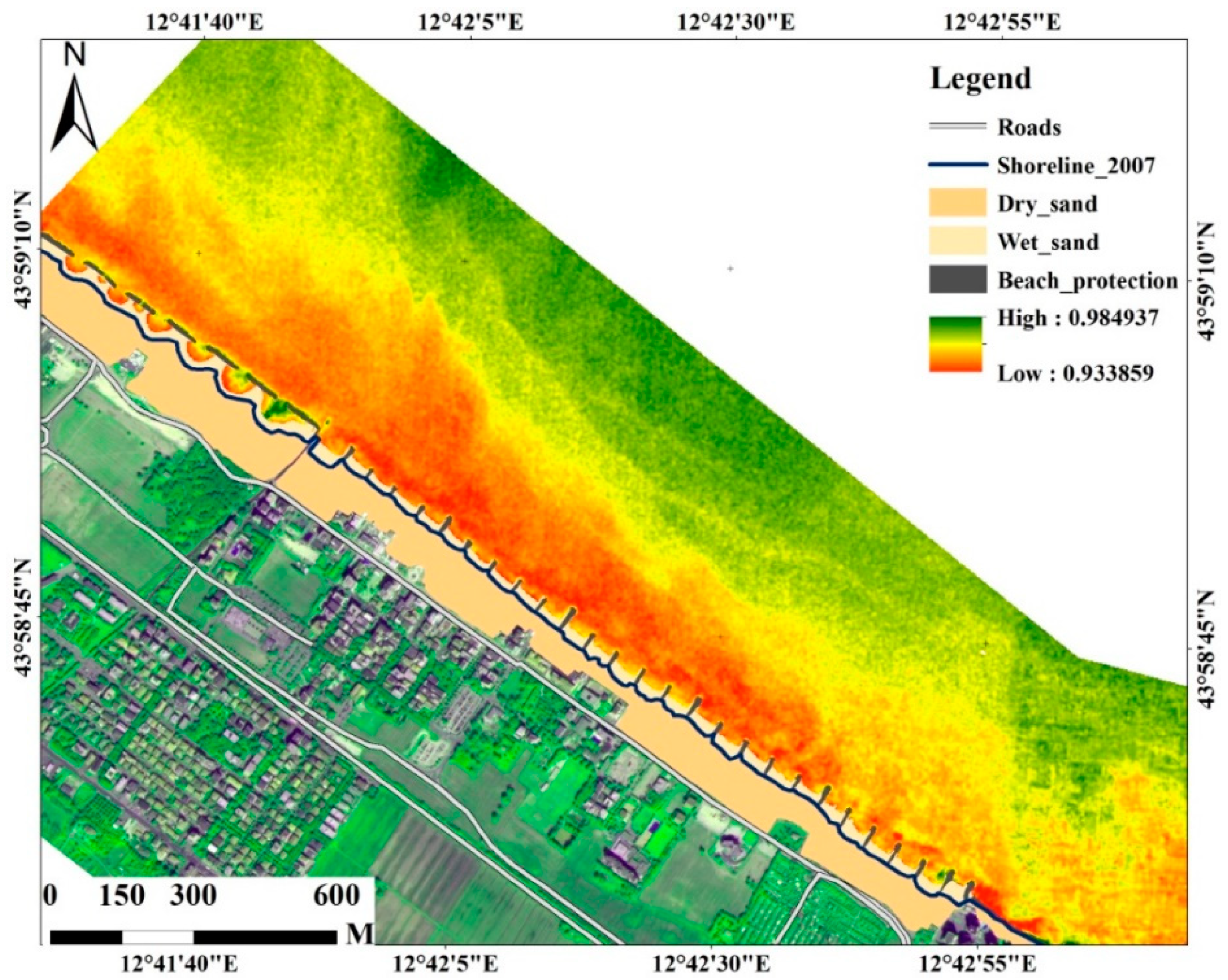
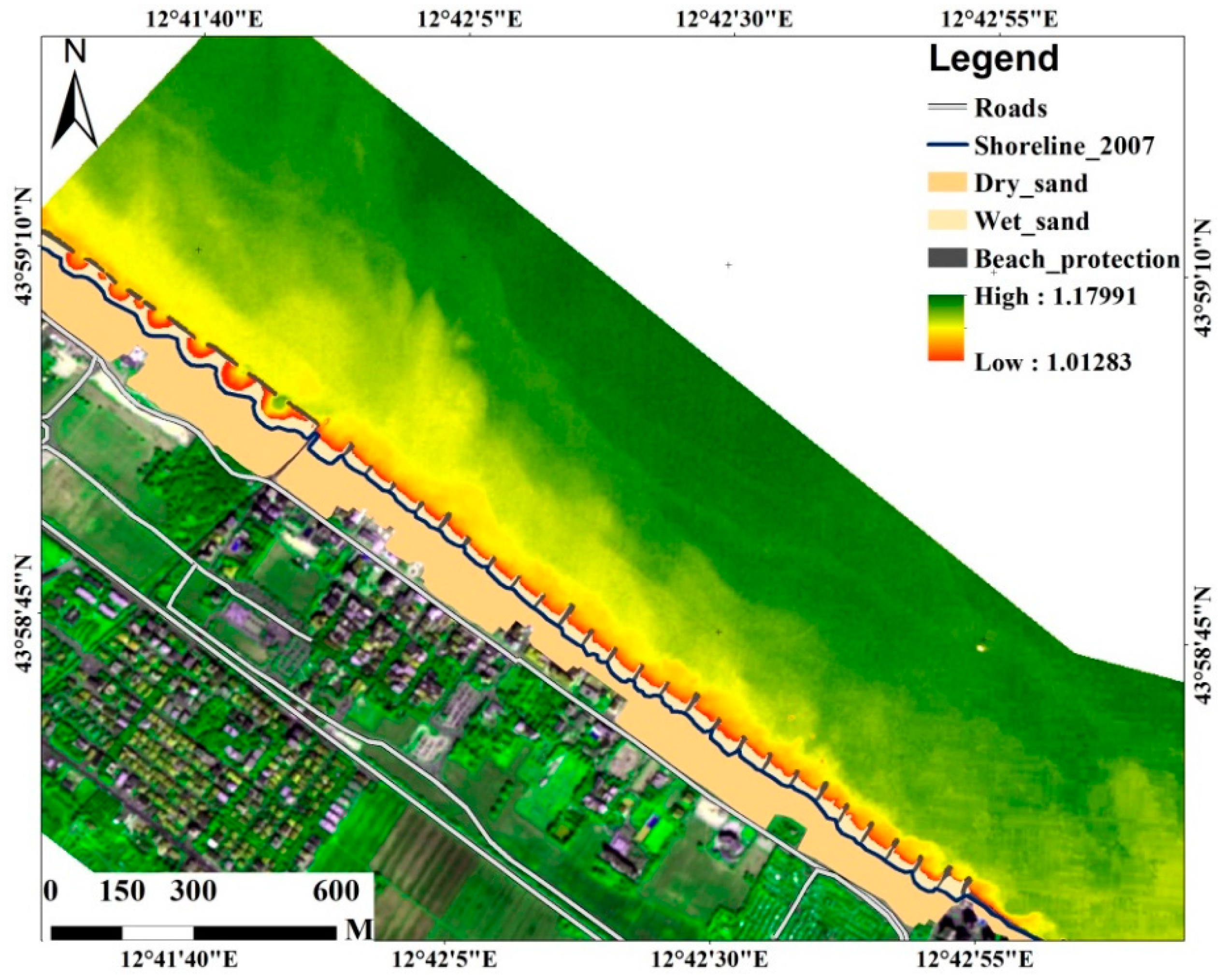
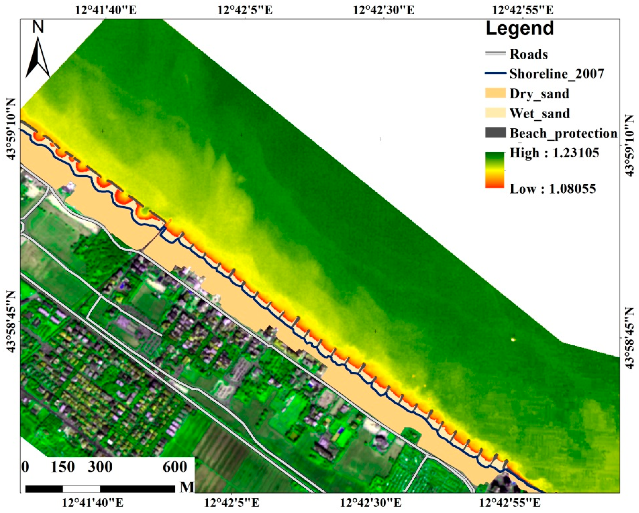
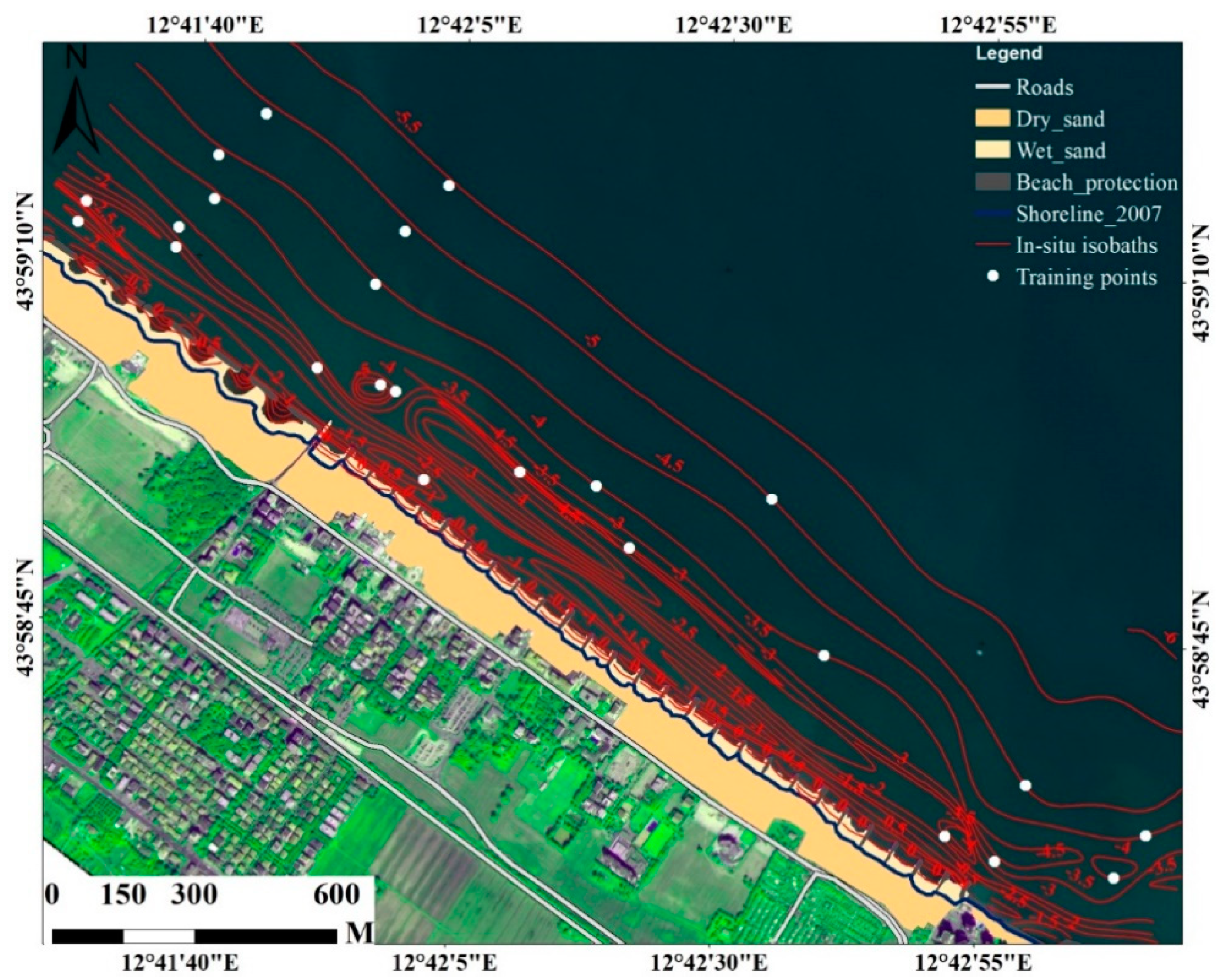
Land-Water Separation and Relative SDB

A line was interpolated on the near infrared band (Figure 3) of the satellite image to extract a threshold value used to separate the land and water pixels for the blue and green bands. The water and land pixels are easily identified in the near infrared image—the smooth (fluctuating) region with low (high) values represents water (land).

Each pixel in three bands has been converted into floating-point representation, which allows the data to support a wide range of digital numbers in big decimal representation. The band ratios (ln(blue)/ln(green), ln(green)/ln(red) and ln(blue)/ln(red)) were determined following the application of a low-pass three-by-three (kernel size 3 × 3) filter over the data. This process has the advantage of smoothing the water part of red, green, and blue bands. The results of the band ratios provide a relative SDB estimation, indicating the qualitative variation of water depth (Figure 4, Figure 5 and Figure 6).

It is important to determine the extinction depth beyond which the relative bathymetry is not reliable. This operation is performed by establishing a regression relationship between in situ known bathymetry and relative SDB. On this in situ bathymetry, 25 points were digitalized by taking into account the variation of water depths as well as the variation of water transparency (Figure 7).

Available in situ bathymetry was limited to 6 m; this led us to restrict our analysis to this water depth. We noted that some points have the same water depth but different relative SDB and did not allow for the determination of extinction depth; for this reason, average mean values were computed and a regression relationship was established on seven points (Figure 8). The extinction depth was identified at 5 m water depth for all band ratios analyzed in the current study. Further analyses to determine absolute SDB were conducted on six points, which presented a good relationship between in situ data and relative SDB.

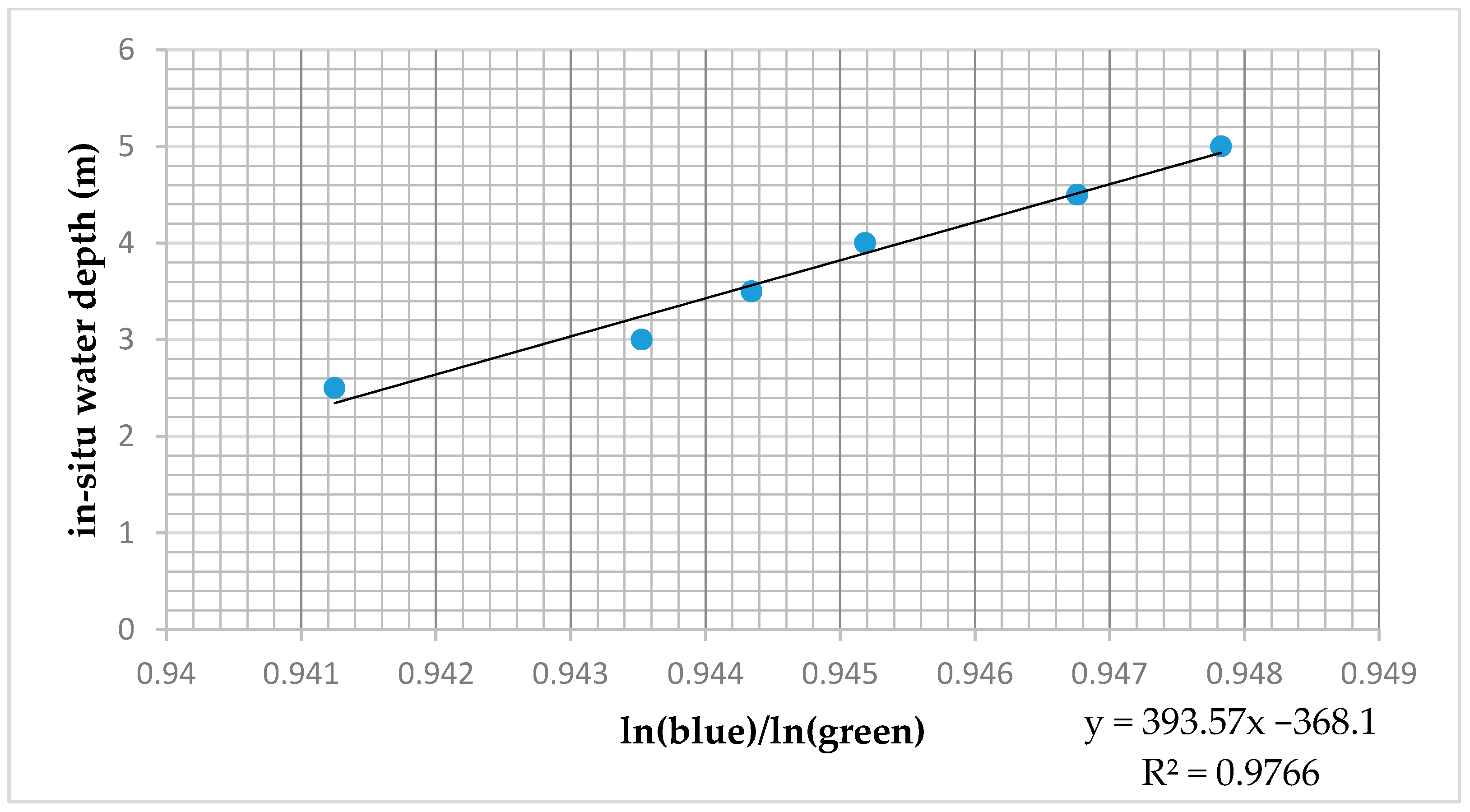
Calibration of Relative SDB

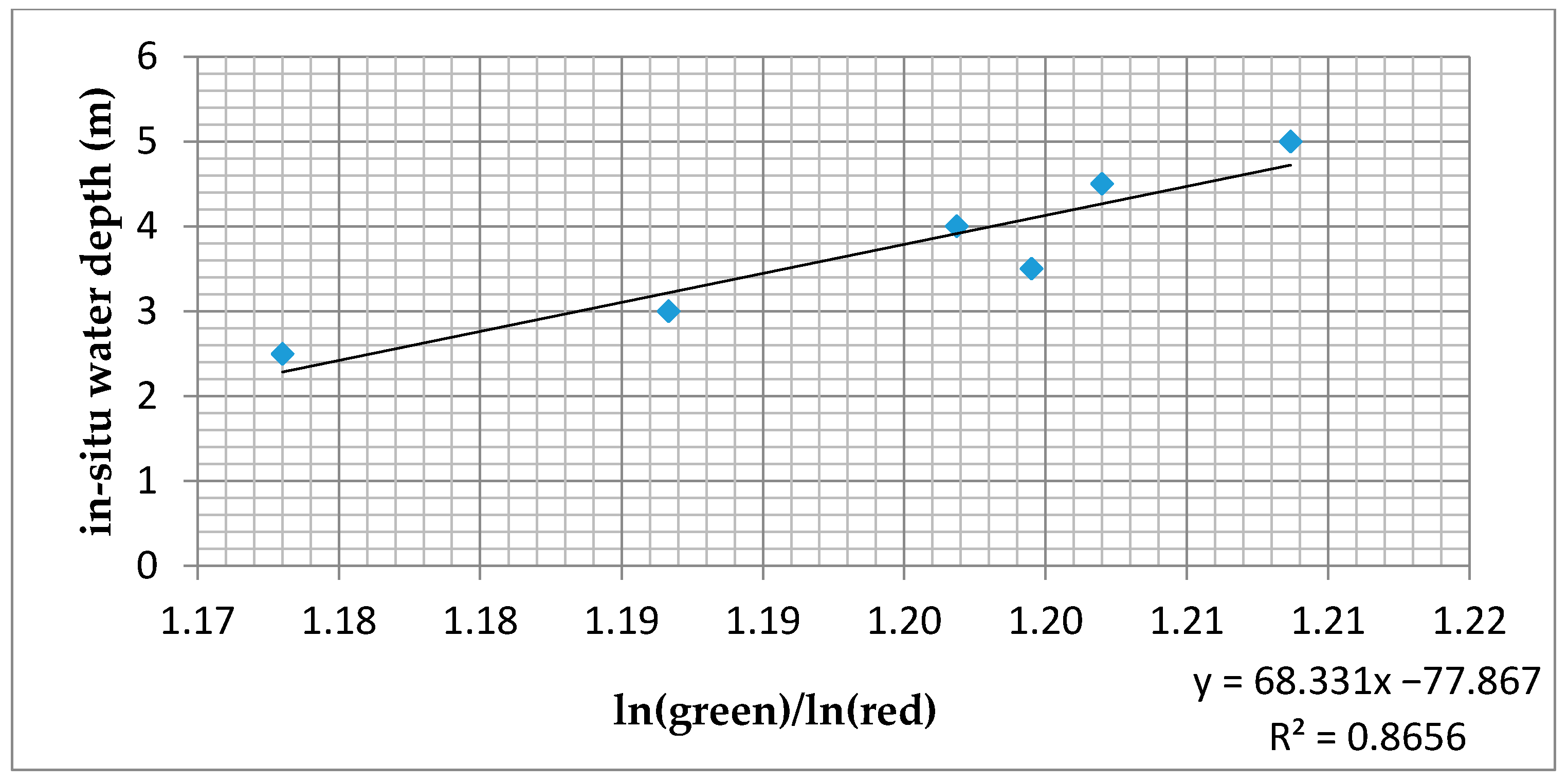
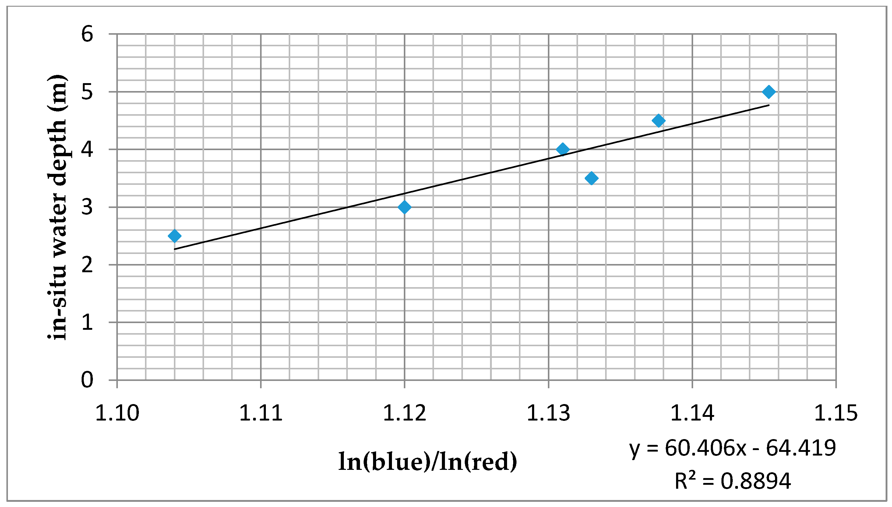
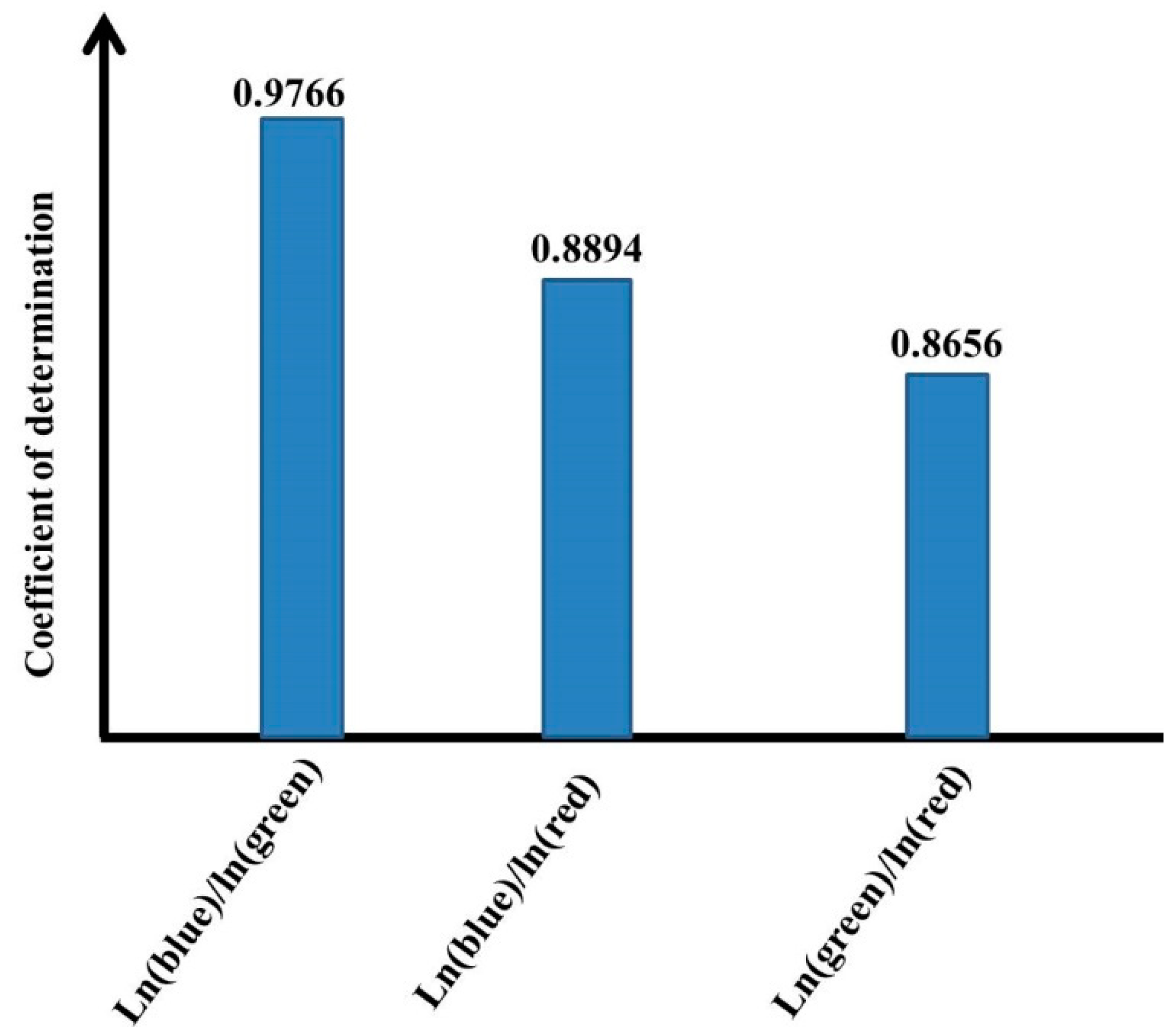
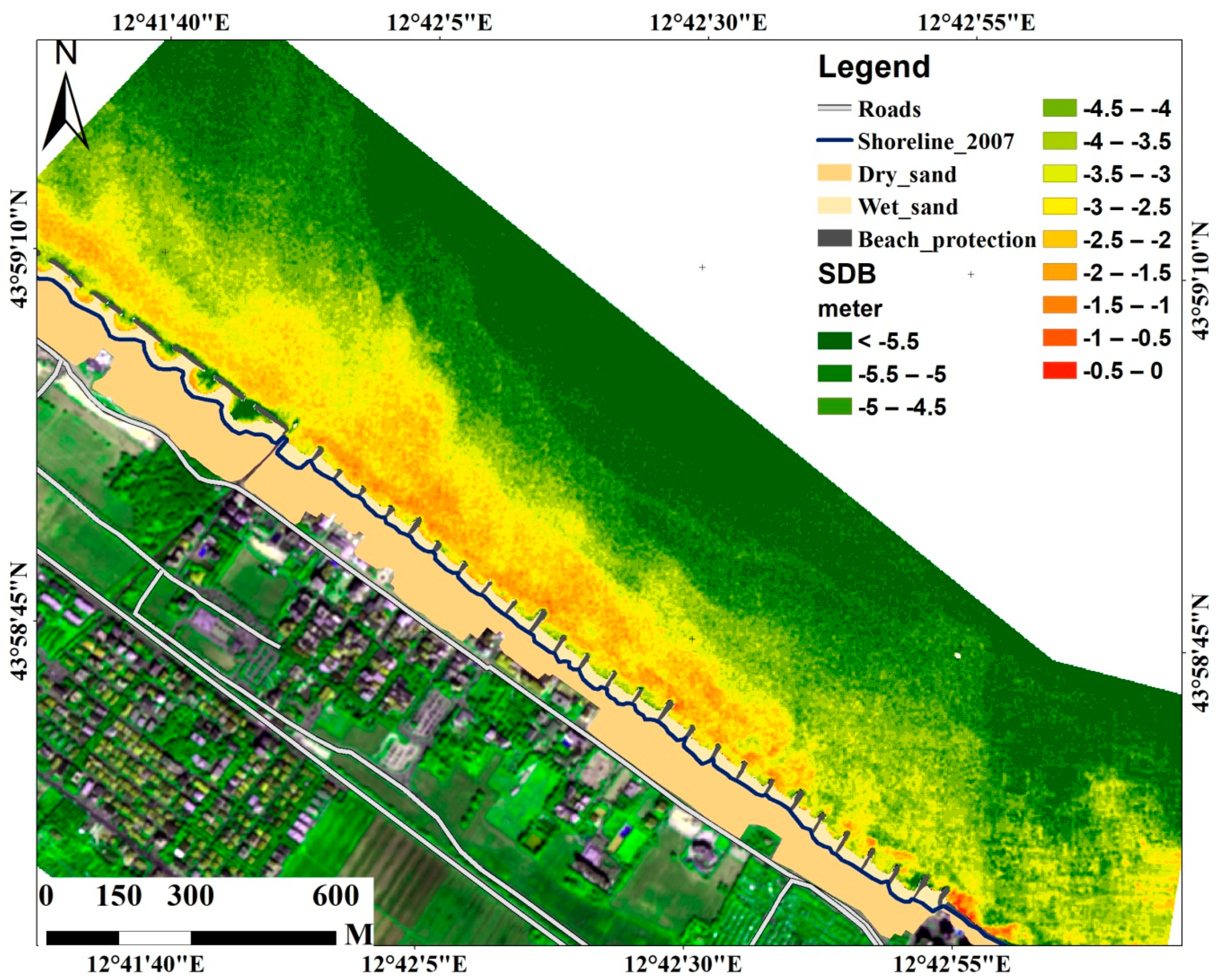
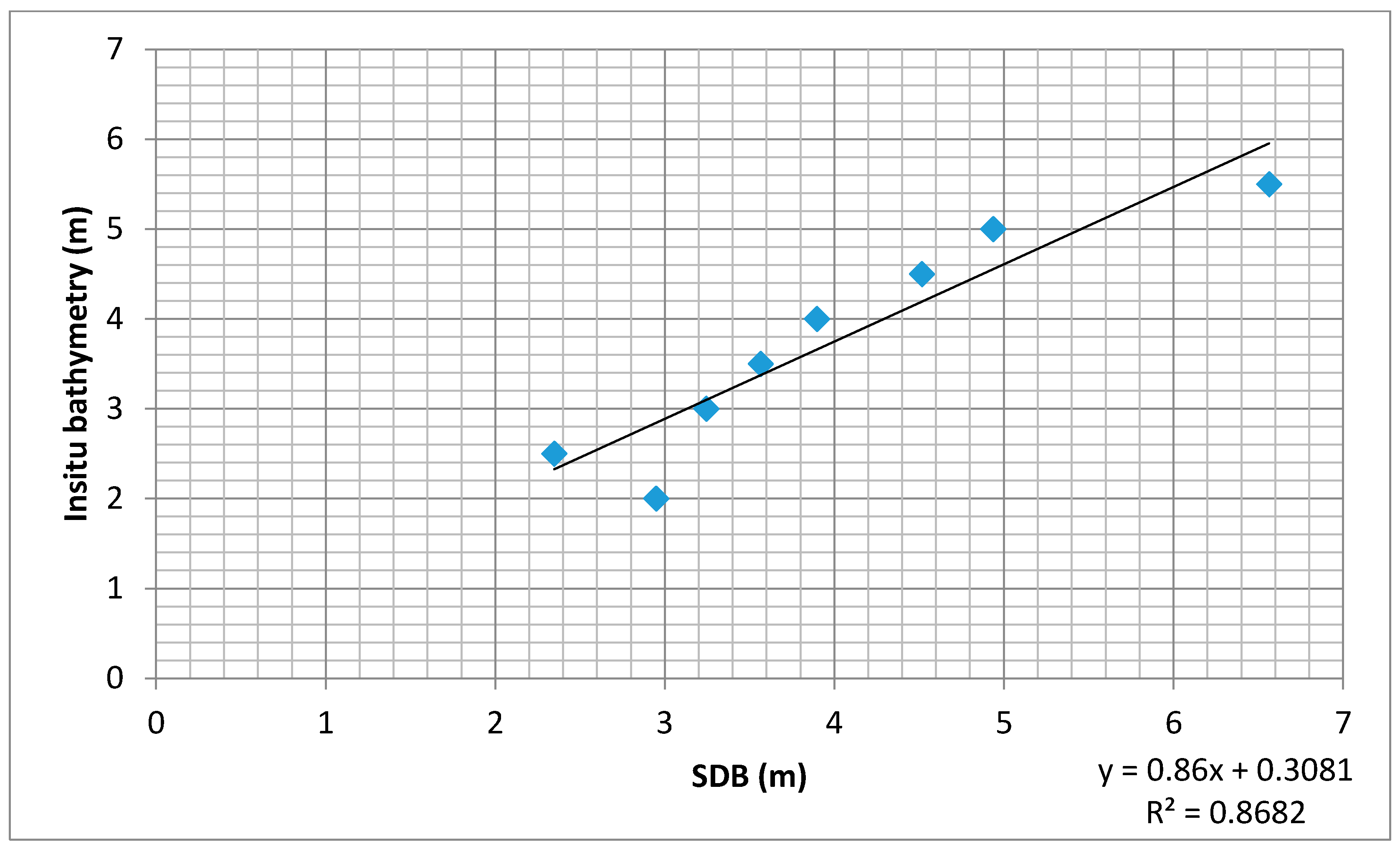
Log-band ratio method

In order to obtain absolute bathymetry, we needed to reference the relative bathymetry to the local datum. This process requires local information obtained from in situ bathymetry survey data. In the current study, we used information collected during a field survey conducted in November 2007 on the Coast of Misano Adriatico. The data were provided by local municipality. We digitized 25 points on the basis of the location of field data isobaths and the optical variation (bright and dark areas) of the water. These training points were homogeneously chosen on in situ data with water depth ranging from 0.5 to 6 m, and with some points having the same water depth values. Figure 9 represents the estimation of vertical reference parameters for 6 point average values computed from 25 points and relative SDB (ln(blue)/ln(green)). This process was executed in Microsoft Excel, where the constant used to scale the ratio to the depth (m1 = 393.57) and the offset for the depth of z = 0 (m0 = −368.1) were determined. These values were integrated into Equation (5) to compute the absolute water depth, as described in Equation (8).

$$Z=-393.57\times \frac{\ln \left(\mathrm{blue}\right)}{\ln \left(\mathrm{green}\right)}+368.1$$

(8)

OBRA method

Although the log-band ratio method uses a single band pair, the OBRA method explores all possible pair bands and chooses those that exhibit a strong correlation between in situ water depths and their relative SDB values. This was performed by estimating R² between the band ratios and in-situ bathymetry (Figure 10, Figure 11 and Figure 12), whereby the band ratios less sensitive to the effect of substrate variability [45] presented a highly linear relationship with the in situ water depth information (Figure 12).

The advantage of using OBRA method in turbid water is that by analyzing water reflectance of a large number of bands, we obtained information on the effect of accumulation and sediment loss on the seabed topography, which can be identified by using one pair band. This was due by the fact that light propagation in shallow water is more prominent at low wavelength bands compared to high wavelength bands.

In addition to the relative SDB obtained from the ln(blue)/ln(green), additional two band ratios (ln(blue)/ln(red) and ln(green)/ln(red)) were calibrated to the local datum, as expressed in Equations (9) and (10), in order to obtain absolute SDB.

$$Z=-68.331\times \frac{\ln \left(\mathrm{green}\right)}{\ln \left(\mathrm{red}\right)}+77.867$$

(9)

$$Z=-60.406\times \frac{\ln \left(\mathrm{blue}\right)}{\ln \left(\mathrm{red}\right)}+64.419$$

(10)

The common use of blue and green ratio in absolute SDB studies is based on the fact that they can penetration deeper in the water and hence allows offshore bathymetry mapping, which can reach 30 m in very clear water. However the use of blue and red band ratio in shallow turbid water can provide more precise water depth information due to the water reflectance in red enhanced by the presence of sediment particles, normally absorbed by clear water. The results of green and red band ratio will also be analyzed in order to determine which band ratio can be used in such an environment.

3. Results

Two empirical methods, OBRA and log-band ratio, were tested in order to estimate shallow water bathymetry on the coast of Misano Adriatico. The results demonstrate the ability of satellite images to provide water depth information for large near-shoreline areas. The methodological approach adopted helps us to explore information located in different spectral bands.

The procedure involves several pre-processing steps to transform TOA into spectral reflectance, whereby four bands (blue, green, red, and near infrared) were selected to compute different relative SDB, with the eventual computation of absolute SDB (Figure 13 and Figure 14) after the inclusion of survey data.

The relative SDB obtained from the ratio between the blue and green bands using the log-band ratio method (Figure 4) exhibited low values associated with shallow water and high values linked to relatively deep water regions. These values were calibrated and converted into absolute water depth with the use of field data acquired in November 2007 for 25 points within water not deeper than 5.5 m. The results demonstrated variations in water depth with shallow water near the shoreline and deeper offshore (Figure 13).

The OBRA method helped us to explore three spectral bands in the blue, green, and red regions. These bands were used to determine relative SDB values, which were later calibrated to the local datum. Although ln(blue)/ln(green) values exhibited a high determinant coefficient with in situ data, the calibration of ln(blue)/ln(red) and ln(green)/ln(red) provided absolute SDB values (Figure 14) that were strongly correlated with the field data.

We conducted accuracy assessment for absolute SDB obtained in order to determine their precision. For OBRA method, accuracy assessments were performed using Equations (11) and (12) on the available survey data (

Table 2. In situ bathymetry and absolute satellite-derived bathymetry (SDB) depth ranges used for optimal band ratio analysis (OBRA) SDB accuracy assessment.

In Situ Bathymetry (m)	SDB for Blue and Red Bands (m)	SDB for Green and Red Bands (m)
2.5	2.34	2.36
3	3.23	3.24
3.5	4.07	4.18
4	3.98	3.99
4.5	4.31	4.25
5	4.77	4.70
5.5	6.09	5.91

), whereas for the log-band ratio method, accuracy assessment was conducted by determining the relationship between the two datasets (Figure 15).

$$R^2=1-\frac{{\sum }_i{\left(Zi-SDBi\right)}^2}{{\sum }_i{\left(Zi-Zm\right)}^2}$$

(11)

$$RMSE=\sqrt{\frac{1}{n}{\sum }_{i=1}^n{\left(Zi-SDBi\right)}^2}$$

(12)

where SDB is satellite-derived bathymetry, Z represents in situ water depth, Zm represents in situ water depth mean value, i represents water depth level, and n is the number of data points.

The absolute SDB exhibited root mean square error (RMSE) values of 0.32 and 0.352 m for SDB computed using blue/red and green/red bands, respectively, and 0.518 m for SDB computed using blue and green bands (

Table 3. Validation error statistics for log-band ratio and OBRA SDB methods.

Statistics	Log-Band Ratio Method Blue and Green Bands	OBRA Method
		Blue and Red Bands	Green and Red Bands
R2	0.8682	0.9108	0.8927
RMSE (m)	0.518	0.32	0.352

). This demonstrated the strong performance of the OBRA method, using blue and red bands, in highly dynamic and turbid water.

The results demonstrate the good correlation of the two methods with in situ water depth. Moreover, a limited difference was observed close to the shoreline, where the presence of suspended sediments can often be a source of errors, particularly in the northwest area, where beach nourishment sediments were observed in the water (Figure 1). In general, the derived bathymetry provided key information on depth variation in this shallow water, with high depth in the south alongside the Porto Verde Marina Resort, as well as in the central-eastern region of the study area.

4. Discussion

The current study presented the first SDB investigation on the highly dynamic coast of Misano Adriatico using multispectral satellite imagery. The well-known empirical approaches of Stumpf et al. [28] and Legleiter et al. [43] were tested for bathymetry mapping and subsequently applied to TOA reflectance using data acquired in turbid water. We limited our study to shallow water not deeper than 5.5 m; this depth range was identified as highly dynamic with turbid water. The study was conducted in order to evaluate the potential of SDB in vulnerable coastal areas affected by erosion and accretion processes.

The empirical approaches adopted for estimating bathymetry in this area were fast and relied on a small amount of training field data. They explored information saved in different spectral bands and chose the bands less influenced by bottom type variabilities, thus improving the quality of the results compared to traditional methods. These approaches relied on attenuation of the light through the water column and the surface water reflectance. However this reflectance can be affected by water composition such as finer materials resulting from anthropic activities or material used for the beach nourishment.

The results obtained using three spectral bands (green, blue, and red) can be enhanced by using multispectral satellite images such of Copernicus Sentinel-2A and Sentinel-2B, which have 13 bands; Landsat 8, Operational Land Imager (OLI), which has 9 bands; or DigitalGlobe’s Worldview-2/3, which have 8 bands. The advantage of having a lot of bands is that the effect of water turbidity on light propagation in shallow water is more prominent at short wavelength bands compared to long wavelength bands. By analyzing surface water reflectance of all those bands, it becomes possible to investigate the impact of turbid water on remote sensing bathymetry mapping.

5. Conclusions

The first objective of the current study was to explore the potential of empirical SDB methods in highly dynamic turbid water. To achieve this, we analyzed QuickBird satellite image acquired over the coastal city of Misano Adriatico using Stumpf et al.’s [28] and Legleiter et al.’s [43] methods. A series of pre-processing steps were applied for the satellite image in order to eliminate atmospheric effects and obtain TOA reflectance, which was subsequently processed to extract relative SDB for near offshore water. Next, this relative SDB was calibrated to the local datum by incorporating in situ water depth in order to obtain absolute SDB. The results demonstrated the ability of satellite images to provide water depth information in shallow water.

The second objective was to determine which empirical method between these two analyzed can provide more accurate results in turbid water. To do so, we conducted accuracy assessment for absolute SDB obtained from log-band ratio and OBRA methods. The results showed that OBRA performed better in such an environment. In addition, OBRA method results were analyzed in order to determine the band ratio which provided more accurate absolute SDB. The RMSE and R² values obtained showed that blue and red band ratio performed better.

The results demonstrated the ability of multispectral images to provide water depth information, particularly in shallow turbid water where red and other long wavelength bands can be analyzed in order to determine the effects of sediments and coastal erosion on seabed topography. This methodology can help coastal geomorphologists who use orthophotographs acquired using sensors fixed on drones to extend their studies on bathymetry and water quality. Information provided by SDB can help people involved in coastal area planning in finding solutions for the impact of climate change.

References

1. Pikelj, K.; Juračić, M. Eastern Adriatic Coast (EAC). Geomorphology and Coastal Vulnerability of a Karstic Coast. J. Coast. Res. 2013, 29, 944–957. [Google Scholar] [CrossRef]
2. Cohen, J.E.; Small, C.; Mellinger, A.; Gallup, J.; Sachs, J. Estimates of coastal populations. Science 1997, 278, 1209–1213. [Google Scholar] [CrossRef]
3. Mohanty, P.K.; Panda, U.S.; Pal, S.R.; Mishra, P.K. Monitoring and management of environmental changes along the Orissa coast. J. Coast. Res. 2008, 24, 13–27. [Google Scholar] [CrossRef]
4. Brommer, M.B.; Bochev-van der Burgh, M.L. Sustainable Coastal Zone Management: A Concept for Forecasting Long-Term and Large-Scale Coastal Evolution. J. Coast. Res. 2009, 25, 181–188. [Google Scholar] [CrossRef]
5. Bayram, B.; Seker, D.Z.; Acar, U.; Yuksel, Y.; Guner, A.H.A.; Cetin, I. An Integrated Approach to Temporal Monitoring of the Shoreline and Basin of Terkos Lake. J. Coast. Res. 2013, 29, 1427–1435. [Google Scholar] [CrossRef]
6. Fumagalli, E.; Bibuli, M.; Caccia, M.; Zereik, E.; Fabrizio Del, B.; Gasperini, L.; Giuseppe, S.; Bruzzone, G. Combined Acoustic and Video Characterization of Coastal Environment by means of Unmanned Surface Vehicles. In Proceedings of the 19th World Congress, The International Federation of Automatic Control, Cape Town, South Africa, 24–29 August 2014. [Google Scholar]
7. Kum, B.-C.; Shin, D.H.; Lee, J.H.; Moh, T.J.; Jang, S.; Lee, S.Y.; Cho, J.H. Monitoring Applications for Multifunctional Unmanned Surface Vehicles in Marine Coastal Environments. J. Coast. Res. 2018, 85, 1381–1385. [Google Scholar] [CrossRef]
8. Bibuli, M.; Bruzzone, G.; Caccia, M.; Fumagalli, E.; Saggini, E.; Zereik, E. Unmanned Surface Vehicles for Automatic Bathymetry Mapping and Shores’ Maintenance. In Oceans Taipei; IEEE: Piscataway, NJ, USA, 2014. [Google Scholar] [CrossRef]
9. Bannari, A.; Kadhem, G. MBES-CARIS data validation for bathymetric mapping of shallow water in the kingdom of Bahrain on the Arabian Gulf. Remote Sens. 2017, 9, 385. [Google Scholar] [CrossRef] [Green Version]
10. Anderson, J.T.; Holliday, D.V.; Kloser, R.; Reid, D.G.; Simard, Y. Acoustic seabed classification: Current practice and future directions. ICES J. Mar. Sci. 2008, 65, 1004–1011. [Google Scholar] [CrossRef]
11. Zhao, J.; Zhao, X.; Zhang, H.; Zhou, F. Shallow Water Measurements Using a Single Green Laser Corrected by Building a Near Water Surface Penetration Model. Remote Sens. 2017, 9, 426. [Google Scholar] [CrossRef] [Green Version]
12. Wang, C.K.; Philpot, W.D. Using airborne bathymetric Lidar to detect bottom type variation in shallow waters. Remote Sens. Environ. 2007, 106, 123–135. [Google Scholar] [CrossRef]
13. Horritt, M.S.; Bates, P.D.; Mattinson, M.J. Effects of mesh resolution and topographic representation in 2D finite volume models of shallow water fluvial flow. J. Hydrol. 2006, 329, 306–314. [Google Scholar] [CrossRef]
14. Giordan, D.; Notti, D.; Villa, A.; Zucca, F.; Calò, F.; Pepe, A.; Dutto, F.; Pari, P.; Baldo, M.; Allasia, P. Low cost, multiscale and multi-sensor application for flooded area mapping. Nat. Hazards Earth Syst. Sci. 2018, 18, 1493–1516. [Google Scholar] [CrossRef] [Green Version]
15. Huang, R.; Yu, K.; Wang, Y.; Wang, J.; Mu, L.; Wang, W. Bathymetry of the Coral Reefs of Weizhou Island Based on Multispectral Satellite Images. Remote Sens. 2017, 9, 750. [Google Scholar] [CrossRef] [Green Version]
16. Vos, K.; Harley, M.D.; Splinter, K.D.; Simmons, J.A.; Turner, J.L. Sub-annual to multi-decadal shoreline variability from public available Satellite imagery. Coast. Eng. 2019, 150, 160–174. [Google Scholar] [CrossRef]
17. Dietrich, J.T. Bathymetric Structure-from-Motion: Extracting shallow stream bathymetry from multi-view stereo photogrammetry. Earth Surf. Process. Landf. 2017, 42, 355–364. [Google Scholar] [CrossRef]
18. Agrafiotis, P.; Karantzalos, K.; Georgopoulos, A.; Skarlatos, D. Correcting Image Refraction: Towards Accurate Aerial Image-Based Bathymetry Mapping in Shallow Waters. Remote Sens. 2020, 12, 322. [Google Scholar] [CrossRef] [Green Version]
19. Collings, S.; Botha, E.J.; Anstee, J.; Campbell, N. Depth from Satellite Images: Depth Retrieval Using a Stereo and Radiative Transfer-Based Hybrid Method. Remote Sens. 2018, 10, 1247. [Google Scholar] [CrossRef] [Green Version]
20. Jawak, S.D.; Vadlamani, S.S.; Luis, A.J. A Synoptic Review on Deriving Bathymetry Information Using Remote Sensing Technologies: Models, Methods and Comparisons. Adv. Remote Sens. 2015, 4, 147–162. [Google Scholar] [CrossRef] [Green Version]
21. Leal Alves, D.C.; Espinoza, J.M.A.; Albuquerque, M.G.; Silva, M.B.; Fontoura, J.S.; Serpa, C.; Weschenfelder, J. Bathymetry estimation by orbital data of OLI sensor: A case study of the Rio Grande harbor, southern Brazil. J. Coast. Res. 2018, 85, 51–55. [Google Scholar] [CrossRef]
22. Polcyn, F.C.; Brown, W.L.; Sattinger, I.J. The Measurement of Water Depth by Remote Sensing Techniques; Institute of Science technology, Michigan Technological University: Ann Arbor, MI, USA, 1970. [Google Scholar]
23. Hamylton, S.M.; Hedley, J.D.; Beaman, R.J. Derivation of high-resolution bathymetry from multispectral satellite imagery: A comparison of empirical and optimisation methods through geographical error analysis. Remote Sens. 2015, 7, 16257–16273. [Google Scholar] [CrossRef] [Green Version]
24. Dekker, A.G.; Phinn, S.R.; Anstee, J.; Bissett, P.; Brando, V.E.; Casey, B.; Fearns, P.R.; Hedley, J.; Klonowski, W.M.; Lynch, M. Intercomparison of shallow water bathymetry, hydro-optics, and benthos mapping techniques in Australian and Caribbean coastal environments. Limnol. Oceanogr. Methods 2011, 9, 396–425. [Google Scholar] [CrossRef] [Green Version]
25. Guzinski, R.; Spondylis, E.; Michalis, M.; Tusa, S.; Brancato, G.; Minno, L.; Hansen, L.B. Exploring the utility of bathymetry maps derived with multispectral satellite observations in the field of underwater archaeology. Open Arch. 2016, 2, 243–263. [Google Scholar] [CrossRef] [Green Version]
26. Lyzenga, D.R. Passive remote-sensing techniques for mapping water depth and Bottom Features. Appl. Opt. 1978, 17, 379–383. [Google Scholar] [CrossRef]
27. Lyzenga, D.R. Remote sensing of Bottom Reflectance and water attenuation parameters in shallow water using Aircraft and Landsat data. Int. J. Remote Sens. 1981, 2, 71–82. [Google Scholar] [CrossRef]
28. Stumpf, R.P.; Holderied, K.; Sinclair, M. Determination of water depth with high-resolution satellite imagery over variable bottom types. Limnol. Oceanogr. 2003, 48, 547–556. [Google Scholar] [CrossRef]
29. Mishra, D.; Narumalani, S.; Lawson, M.; Rundquid, D. Bathymetric mapping Using IKONOS Multispectral data. GISci. Remote Sens. 2004, 41, 301–321. [Google Scholar] [CrossRef]
30. Lesser, M.P.; Mobley, C.D. Bathymetry, water optical properties, and benthic classification of coral reefs using hyperspectral remote sensing imagery. Coral Reefs 2007, 26, 819–829. [Google Scholar] [CrossRef]
31. Poliyapram, V.; Raghavan, V.; Metz, M.; Delucchi, L. Implementation of algorithm for satellite-derived bathymetry using open Source GIS and evaluation for tsunami simulation. Int. J. Geo-Inf. 2017, 6, 89. [Google Scholar] [CrossRef] [Green Version]
32. Muzirafuti, A.; Crupi, A.; Lanza, S.; Barreca, G.; Randazzo, G. Shallow water bathymetry by satellite image: A case study on the coast of San Vito Lo Capo Peninsula, Northwestern Sicily, Italy. In Proceedings of the IMEKO TC-19 International Workshop on Metrology for the Sea, Genoa, Italy, 3–5 October 2019. [Google Scholar]
33. Mavraeidopoulos, A.K.; Oikonomou, E.; Palikaris, A.; Poulos, S. A Hybrid Bio-Optical Transformation for Satellite Bathymetry Modeling Using Sentinel-2 Imagery. Remote Sens. 2019, 11, 2746. [Google Scholar] [CrossRef] [Green Version]
34. Eugenio, F.; Marcello, J.; Martin, J. High-resolution maps of bathymetry and benthic habitats in shallow-water environments using multispectral remote sensing imagery. IEEE Trans. Geosci. Remote Sens. 2015, 53, 3539–3549. [Google Scholar] [CrossRef]
35. Lyzenga, D.R. Shallow-water bathymetry using combined lidar and passive multispectral scanner data. Int. J. Remote Sens. 1985, 6, 115–125. [Google Scholar] [CrossRef]
36. Morel, Y.G.; Favoretto, F. 4SM: A novel self-calibrated algebraic ratio method for satellite-derived bathymetry and water column correction. Sensors 2017, 17, 1682. [Google Scholar] [CrossRef] [PubMed]
37. Bramante, J.F.; Raju, D.K.; Sin, T.M. Multispectral derivation of bathymetry in Singapore’s shallow, turbid waters. Int. J. Remote Sens. 2013, 34, 2070–2088. [Google Scholar] [CrossRef]
38. Legleiter, C.J.; Kinzel, P.J.; Overstreet, B.T. Evaluating the potential for remote bathymetric mapping of a turbid, sand-bed river: 1. Field spectroscopy and radiative transfer modeling. Water Resour. Res. 2011, 47. [Google Scholar] [CrossRef] [Green Version]
39. Joshi, I.D.; DSa, E.J.; Osburn, C.L.; Bianchi, T.S. Turbidity in Apalachicola Bay, Florida from Landsat 5 TM and Field Data: Seasonal Patterns and Response to Extreme Events. Remote Sens. 2017, 9, 367. [Google Scholar] [CrossRef] [Green Version]
40. Gao, B.-C.; Montes, M.J.; Li, R.-R.; Dierssen, H.M.; Davis, C.O. An Atmospheric Correction Algorithm for Remote Sensing of Bright Coastal Waters Using MODIS Land and Ocean Channels in the Solar Spectral Region. IEEE Trans. Geosci. Remote Sens. 2007, 45, 1835–1843. [Google Scholar] [CrossRef]
41. Pike, S.; Traganos, D.; Poursanidis, D.; Williams, J.; Medcalf, K.; Reinartz, P.; Chrysoulakis, N. Leveraging Commercial High-Resolution Multispectral Satellite and Multibeam Sonar Data to Estimate Bathymetry: The Case Study of the Caribbean Sea. Remote Sens. 2019, 11, 1830. [Google Scholar] [CrossRef] [Green Version]
42. Caballero, I.; Stumpf, R.P. Retrieval of nearshore bathymetry from Sentinel-2A and 2B satellites in South Florida coastal waters. Estuar. Coast. Shelf Sci. 2019, 226, 106277. [Google Scholar] [CrossRef]
43. Legleiter, C.J.; Roberts, D.A.; Lawrence, R.L. Spectrally based remote sensing of river bathymetry. Earth Surf. Process. Landf. 2009, 34, 1039–1059. [Google Scholar] [CrossRef]
44. Pe’eri, S.; Parrish, C.; Azuike, C.; Alexander, L.; Armstrong, A. Satellite remote sensing as a reconnaissance tool for assessing nautical chart adequacy and completeness. Mar. Geod. 2014, 37, 293–314. [Google Scholar] [CrossRef]
45. Niroumand-Jadidi, M.; Vitti, A. Optimal band ratio analysis of worldview-3 imagery for bathymetry of shallow rivers (case study: Sarca River, Italy). Int. Arch. Photogramm. Remote Sens. Spat. Inf. Sci. 2016, XLI-B8, 361–365. [Google Scholar] [CrossRef]
46. Perini, L.; Calabrese, L. Le dune costiere dell’Emilia-Romagna: Strumenti di analisi, cartografia ed evoluzione 2010. Studi Costieri 2010, 17, 71–84. [Google Scholar]
47. Perini, L.; Lorito, S.; Calabrese, L. Il Catalogo delle opere di difesa costiera della Regione Emilia Romagna. Studi Costieri 2008, 15, 39–56. [Google Scholar]
48. Armaroli, C.; Ciavola, P.; Perini, L.; Calabrese, L.; Lorito, S.; Valentini, S.; Masina, M. Critical storm thresholds for significant morphological changes and damage along the Emilia-Romagna coast, Italy. Geomorphology 2012, 143, 34–51. [Google Scholar] [CrossRef]
49. Aguzzi, M.; Bonsignore, F.; De Nunzio, N.; Morelli, M.; Paccagnella, T.; Romagnoli, C.; Unguendoli, S. Stato del Litorale Emiliano-Romagnolo al 2012: Erosione e Interventi di Difesa; Agenzia Prevenzione Ambiente Energia Emilia-Romagna: Bologna, Italy, 2016; ISBN 978-88-87854-41-1. [Google Scholar]
50. Montanari, R.; Marasmi, C. New Tools for Coastal Management in Emilia-Romagna, COASTANCE Project; Emilia-Romagna Region: Bologna, Italy, 2012. [Google Scholar]
51. European Space Imaging. Available online: https://www.euspaceimaging.com/ (accessed on 6 September 2018).
52. International Hydrographic Organization. IHO Standards for Hydrographic Surveys (S-44), Special Publication No. 44, 5th ed.; International Hydrographic Bureau: Monaco City, Monaco, 2008; p. 28. [Google Scholar]
53. Malinowski, R.; Groom, G.; Schwanghart, W.; Heckrath, G. Detection and Delineation of Localized Flooding from WorldView-2 Multispectral Data. Remote Sens. 2015, 7, 14853–14875. [Google Scholar] [CrossRef] [Green Version]
54. Krause, K. Radiometric Conversion of QuickBird Data-Technical Note; DigitalGlobe Inc.: Longmont, CO, USA, 2003. [Google Scholar]
55. International Hydrographic Organization, Intergovernmental Oceanographic Commission. The IHO-IOC GEBCO Cook Book; IHO Publication B-11: Monaco City, Monaco, 2018; p. 429, pp.416-IOC Manuals and Guides 63, France, 2018. [Google Scholar]
56. Jensen, J.R. Remote Sensing of the Environment: An Earth Resource Perspective, 2nd ed.; Prentice Hall: Upper Saddle River, NJ, USA, 2007. [Google Scholar]
Figure 1. Map of accumulation and sediment loss over the Port of Riccione during 2006–2012, modified from [49]. It shows the accumulation of sediments on the seabed in the northernmost stretch of the coast of Misano. Aguzzi et al. noted a loss of volume of approximately 24,000 m3 during the same period (2006–2012), 13,000 m3 of which originated from cliffs and 11,000 m3 from the beach and cliffs.
Jmse 08 00126 g001
Figure 2. True-color composite of QuickBird satellite image (acquired 7 September 2007) over Misano Adriatico. Ocean basemap of Italy (A) indicating the location of Misano Adriatico (red dot) and (B) true-color composite of QuickBird satellite image (acquired 7 September 2007) indicating the location of the Rimini-Misano Coast (red rectangle).
Jmse 08 00126 g002
Figure 3. Threshold values extracted from the near infrared (NIR) band on the coast of Misano Adriatico. The interpolated line indicates the area on which offshore and onshore reflectance values were extracted, as presented on the profile. Constant and low values indicate water pixels, whereas high and fluctuant values indicate land pixels.
Jmse 08 00126 g003
Figure 4. Relative satellite-derived bathymetry (SDB) from the ln(blue)/ln(green) band ratio of the QuickBird image, representing very shallow water near the shoreline and relatively deep water. The shoreline (2007) indicates the separation of dry and wet sand for this image taken on 7 September 2007. Note the presence of main roads as well as built-up areas.
Jmse 08 00126 g004
Figure 5. Relative SDB from the ln(blue)/ln(red) band ratio of the QuickBird image, representing very shallow water near the shoreline and relatively deep water. The shoreline (2007) indicates the separation of dry and wet sand for this image taken on 7 September 2007. Note the presence of main roads as well as built-up areas.
Jmse 08 00126 g005
Figure 6. Relative SDB from the ln(green)/ln(red) band ratio of the QuickBird image, representing very shallow water near the shoreline and relatively deep water. The shoreline (2007) indicates the separation of dry and wet sand for this image taken on 7 September 2007. Note the presence of main roads as well as built-up areas.
Jmse 08 00126 g006
Figure 7. Locations of 25 points used for band ratio regression analysis. The black dots represent the points digitalized on different isobaths with known water depth. Note the highly variable seabed topography near the shoreline where the isobaths are too tight.
Jmse 08 00126 g007
Figure 8. Determination of water depth extinction, example for in situ data and relative SDB from the ln(blue)/ln(green) band ratio.
Jmse 08 00126 g008
Figure 9. Vertical referencing parameter and R2 estimated from in situ water depth and relative SDB. Relative SDB values were obtained from the logarithmic expression of the blue and green bands (ln(blue)/ln(green)), whereas in situ water depth values were obtained from in situ bathymetry acquired during November 2007.
Jmse 08 00126 g009
Figure 10. Vertical referencing parameter and R2 estimated from in situ water depth and relative SDB. Relative SDB values were obtained from the logarithmic expression of the green and red bands (ln(green)/ln(red)), whereas in situ water depth values were obtained from in situ bathymetry acquired during November 2007. Note the distribution of points where the influence of particular localized turbidity may be shown by the presence some outliers, especially at 3.5 m water depth.
Jmse 08 00126 g010
Figure 11. Vertical referencing parameter and R2 estimated from in situ water depth and relative SDB. Relative SDB values were obtained from the logarithmic expression of the blue and red bands (ln(blue)/ln(red)), whereas in situ water depth values were obtained from in situ bathymetry acquired during November 2007. Note the distribution of points where the influence of particular localized turbidity may be shown by the presence some outliers, especially at point 3.5 m water depth.
Jmse 08 00126 g011
Figure 12. R2 obtained from ln(blue)/ln(green), ln(green)/ln(red), and ln(blue)/ln(red) band ratios and in situ water depth.
Jmse 08 00126 g012
Figure 13. Absolute SDB, on the coast of Misano Adriatico, extracted from the QuickBird image (acquired on 7 September 2007) using the log-band ratio method. The bathymetry was obtained by calibrating and vertically referencing relative SDB, ln(blue)/ln(green), to the local datum using in situ water depth.
Jmse 08 00126 g013
Figure 14. Absolute SDB, on the coast of Misano Adriatico, extracted from the QuickBird image (acquired on 7 September 2007) using the OBRA method (based on the blue and red bands). The bathymetry was obtained by calibrating and vertically referencing relative SDB, ln(blue)/ln(red), to the local datum using in situ water depth.
Jmse 08 00126 g014
Figure 15. Correlation between in situ bathymetry and SDB obtained using log-band ratio method on the coast of Misano Adriatico. Note that influence of particular localized turbidity on SDB may be demonstrated by the presence of some outliers, especially at water depth of 3 m.
Jmse 08 00126 g015