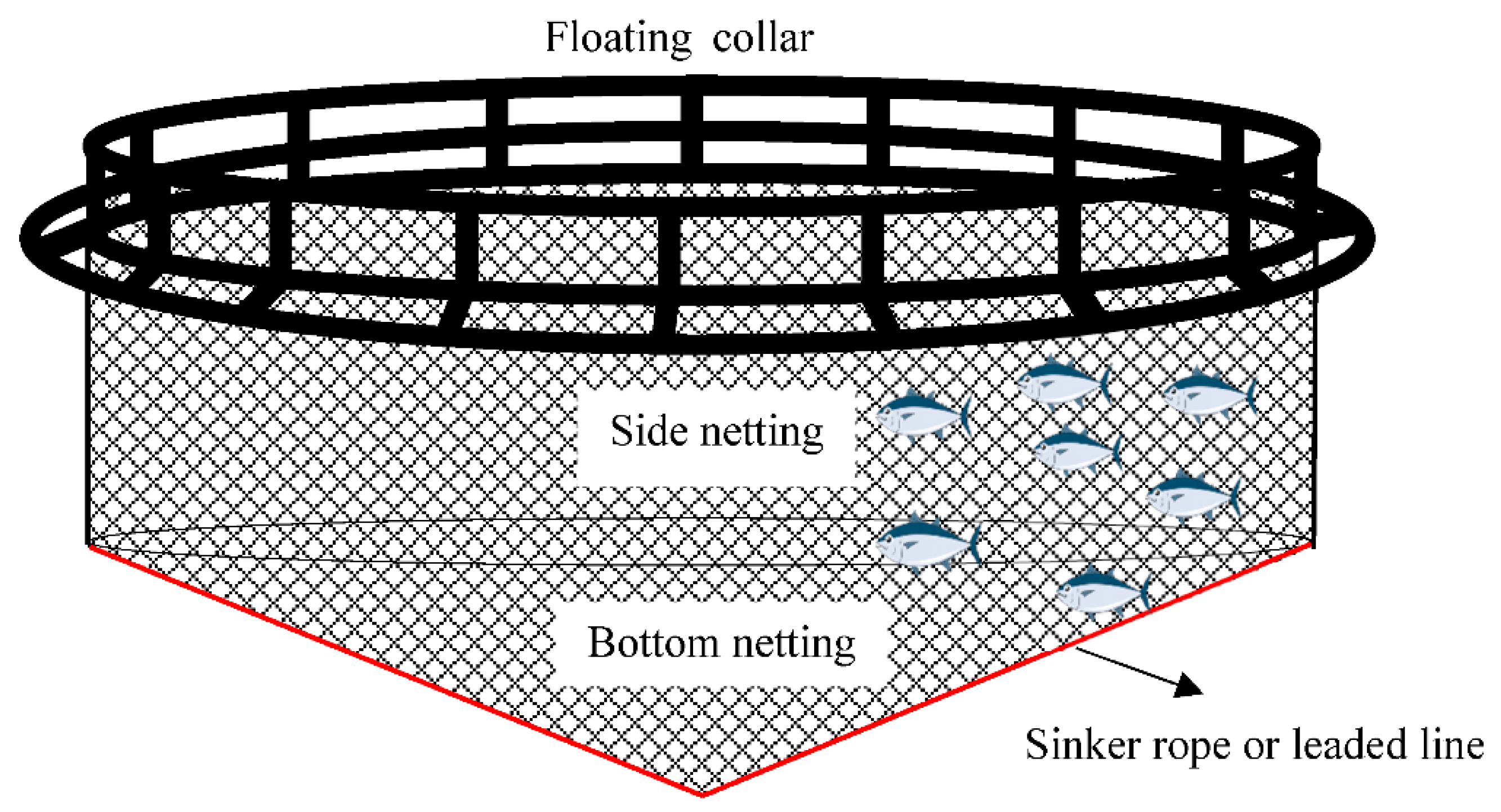
Figure 1.
Schematic diagram of prototype net cage used for farming pacific bluefin tuna.
Figure 1.
Schematic diagram of prototype net cage used for farming pacific bluefin tuna.
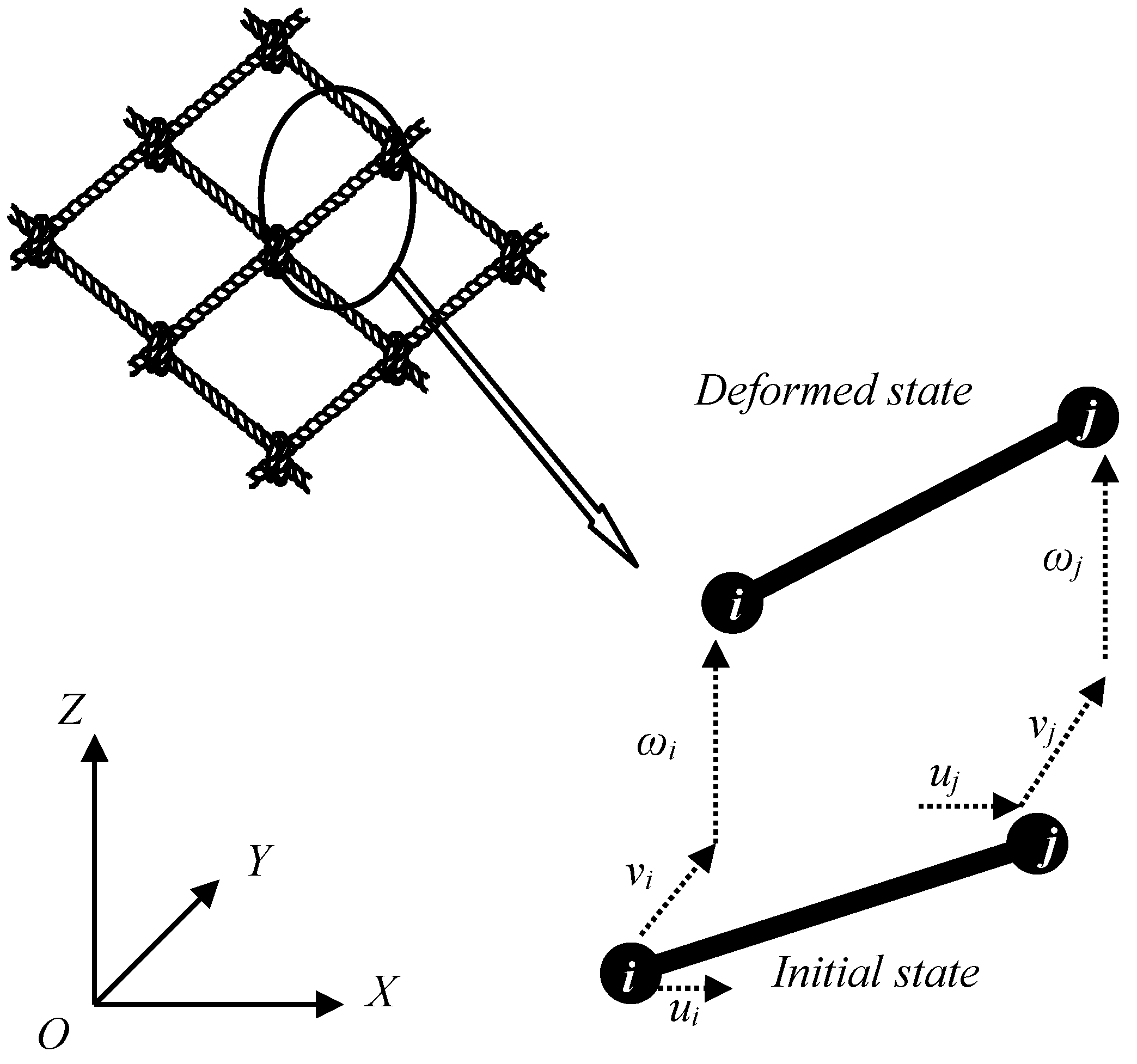
Figure 2.
Diagram of the element motion. X, Y, and Z, are the global system coordinates; u, v, and ω, denote the nodal displacements of an element in the direction of X, Y, and Z axes; and i and j indicate the ends of the element, respectively.
Figure 2.
Diagram of the element motion. X, Y, and Z, are the global system coordinates; u, v, and ω, denote the nodal displacements of an element in the direction of X, Y, and Z axes; and i and j indicate the ends of the element, respectively.
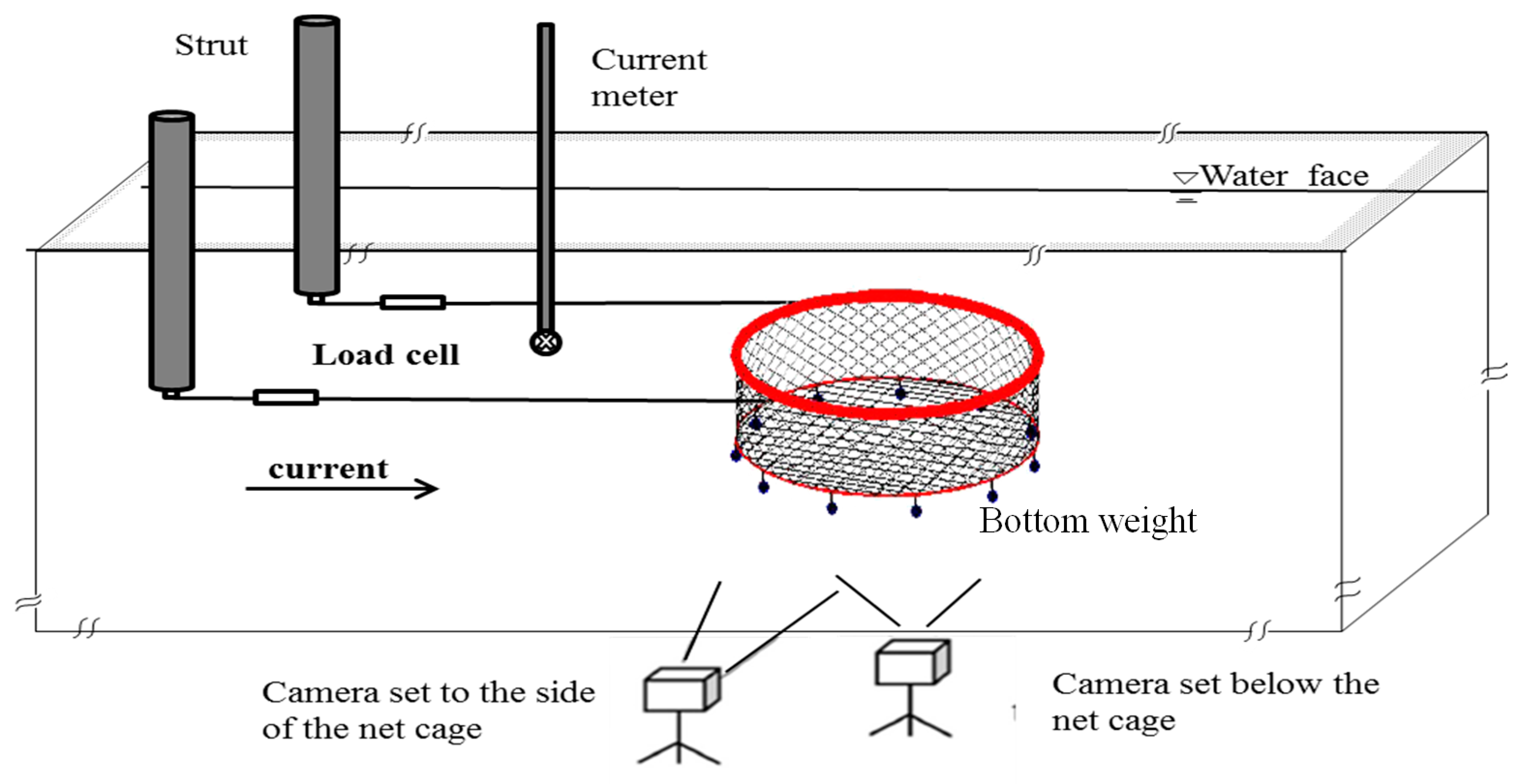
Figure 3.
Schematic of experiment setup.
Figure 3.
Schematic of experiment setup.
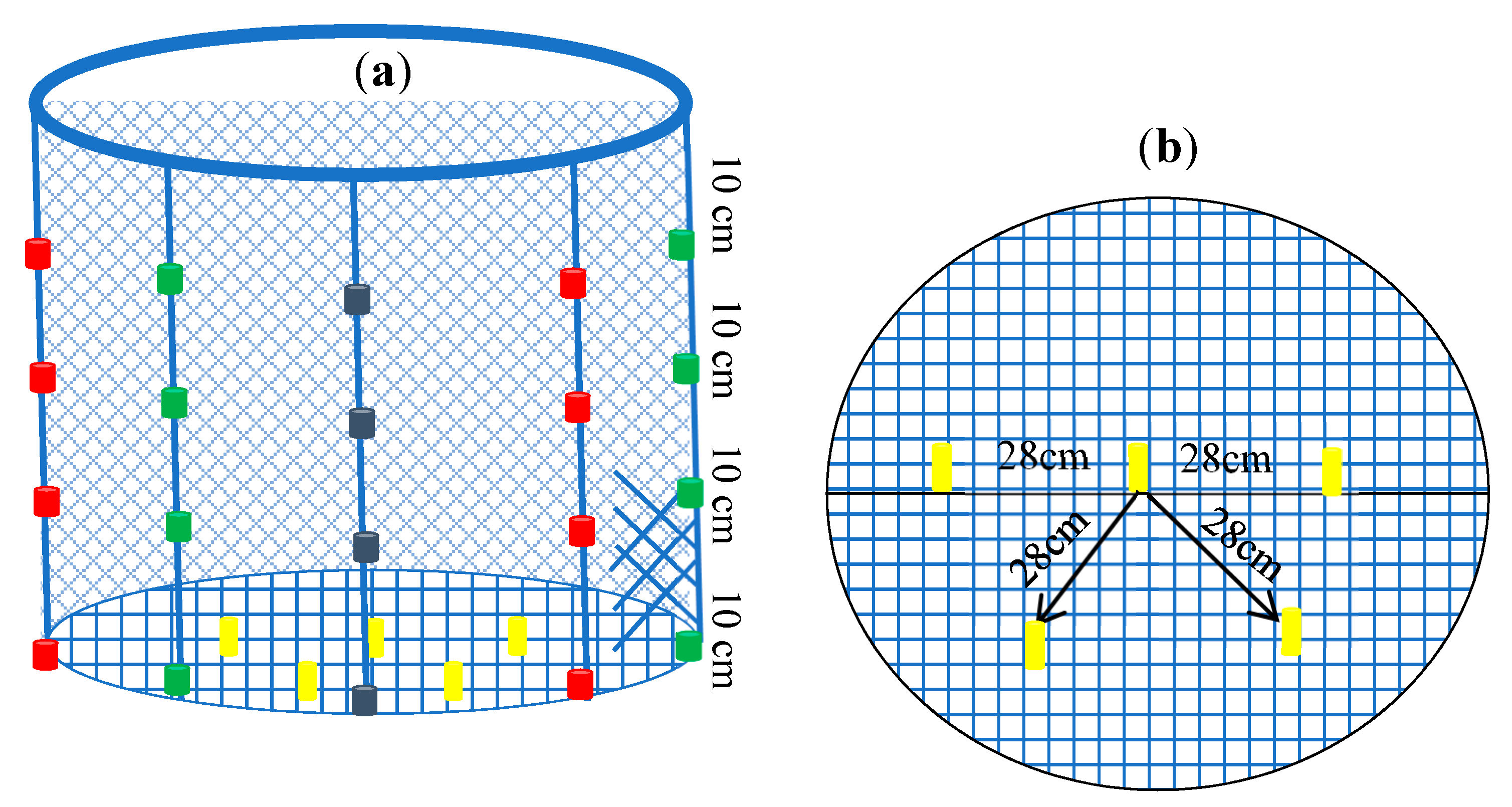
Figure 4.
Placement of light-emitting diode (LED) markers on the side and bottom netting. (a) Side and (b) bottom nettings.
Figure 4.
Placement of light-emitting diode (LED) markers on the side and bottom netting. (a) Side and (b) bottom nettings.
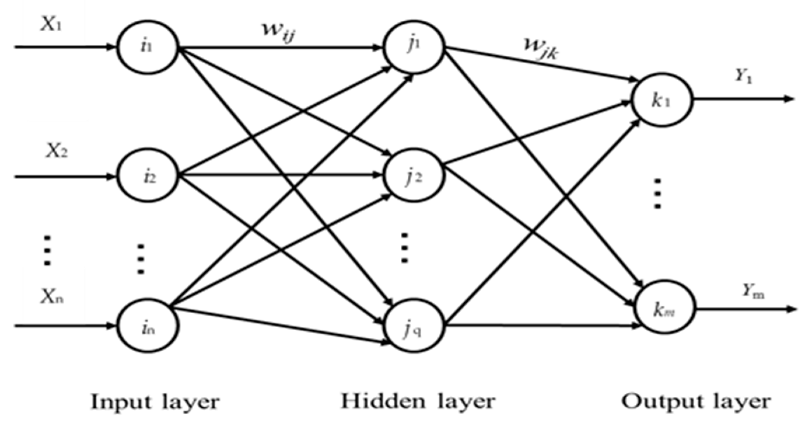
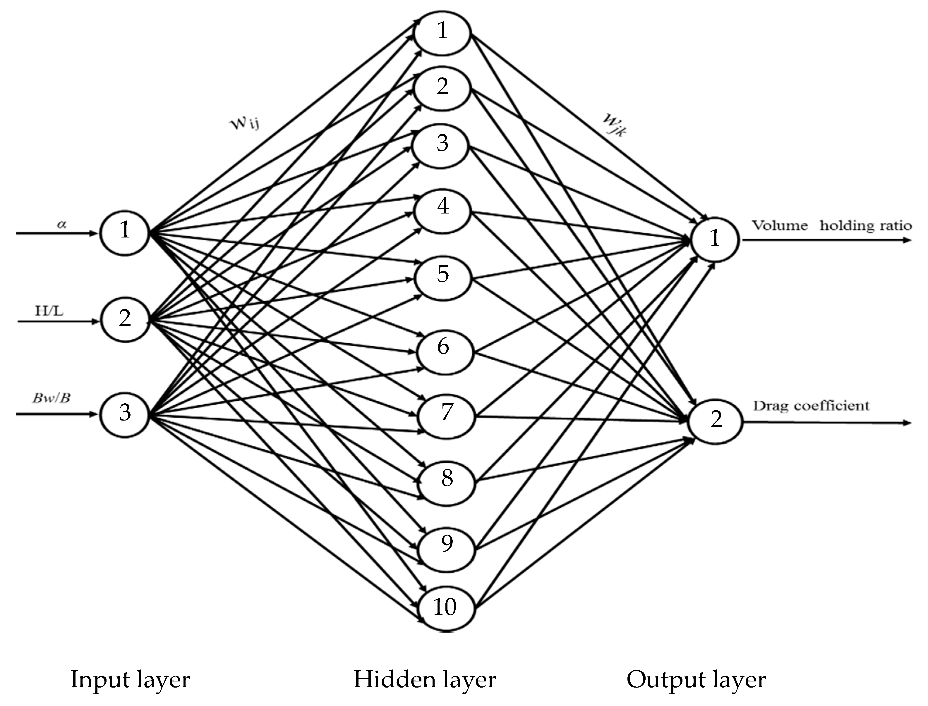
Figure 5.
Topology diagram of backpropagation (BP) neural network.
Figure 5.
Topology diagram of backpropagation (BP) neural network.
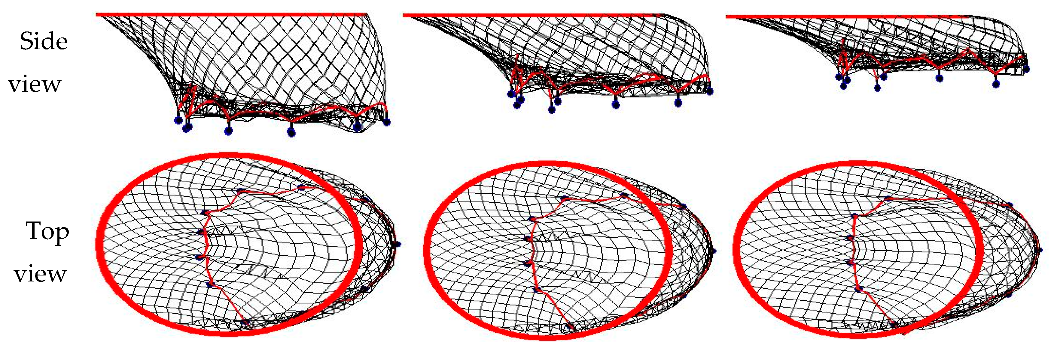
Figure 6.
Equilibrium geometry of the net cage at current speeds of 20, 30, and 40 cm/s.
Figure 6.
Equilibrium geometry of the net cage at current speeds of 20, 30, and 40 cm/s.
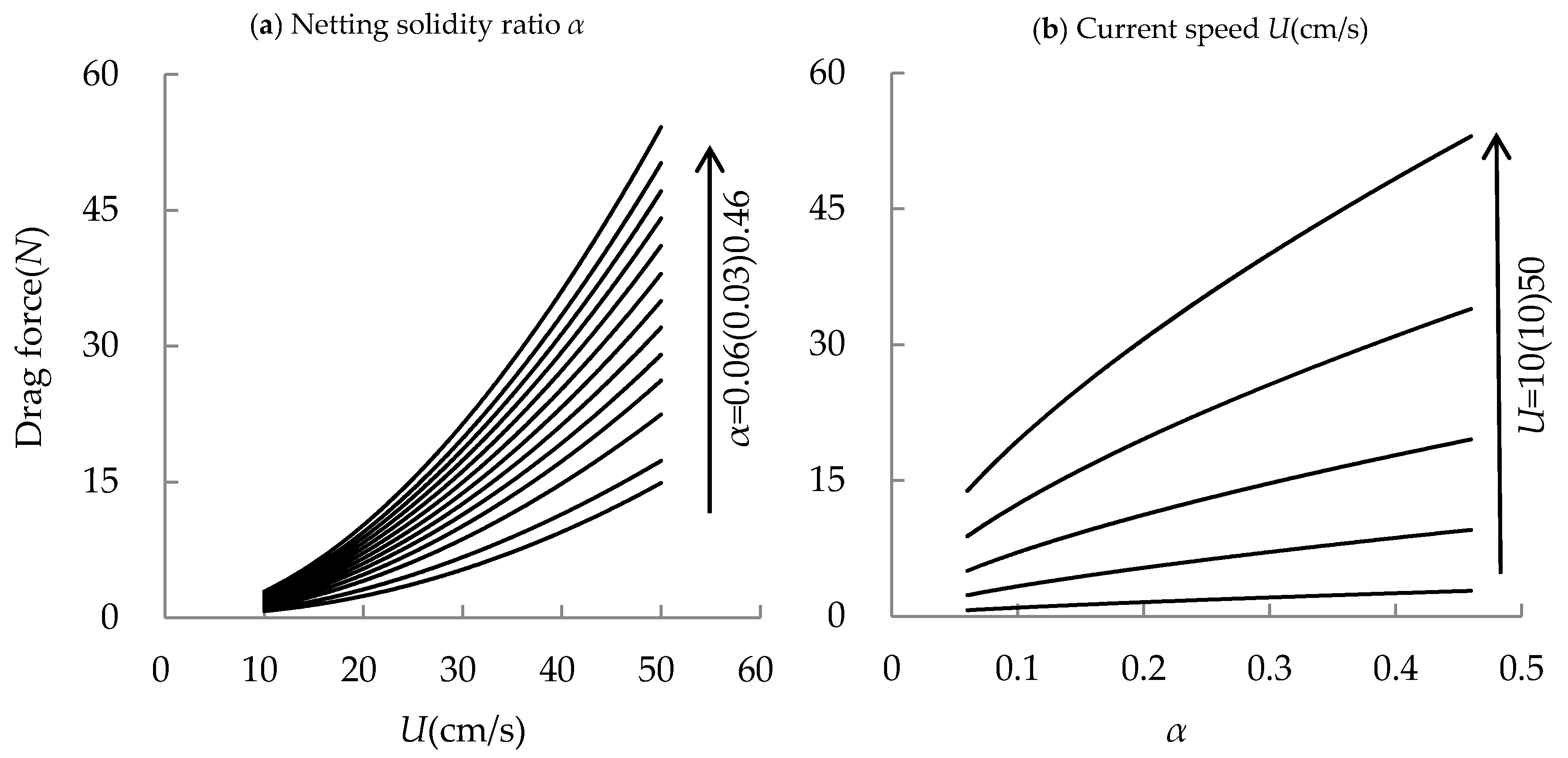
Figure 7.
Relationship of drag force and mesh factor plotted against current speed. (a) the relationship of RD and U for each α; (b) the relationship between RD and α for each U.
Figure 7.
Relationship of drag force and mesh factor plotted against current speed. (a) the relationship of RD and U for each α; (b) the relationship between RD and α for each U.
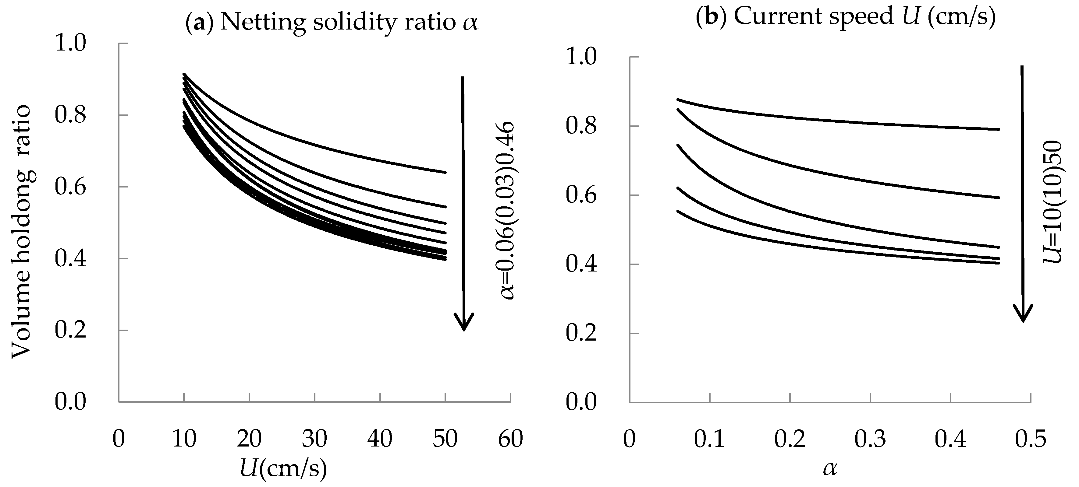
Figure 8.
Relationship of volume holding ratio and mesh factor plotted against current speed. (a) the relationship of Cv and U for each α; (b) the relationship between Cv and α for each U.
Figure 8.
Relationship of volume holding ratio and mesh factor plotted against current speed. (a) the relationship of Cv and U for each α; (b) the relationship between Cv and α for each U.
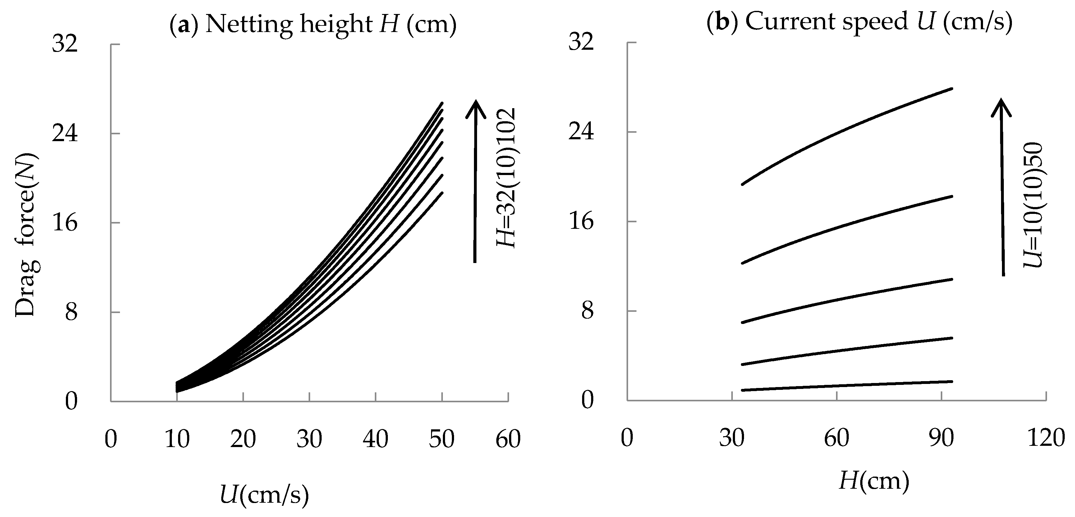
Figure 9.
Relationship of drag force and net depth plotted against current speed. (a) the relationship of RD and U for each H; (b) the relationship between RD and H for each U.
Figure 9.
Relationship of drag force and net depth plotted against current speed. (a) the relationship of RD and U for each H; (b) the relationship between RD and H for each U.
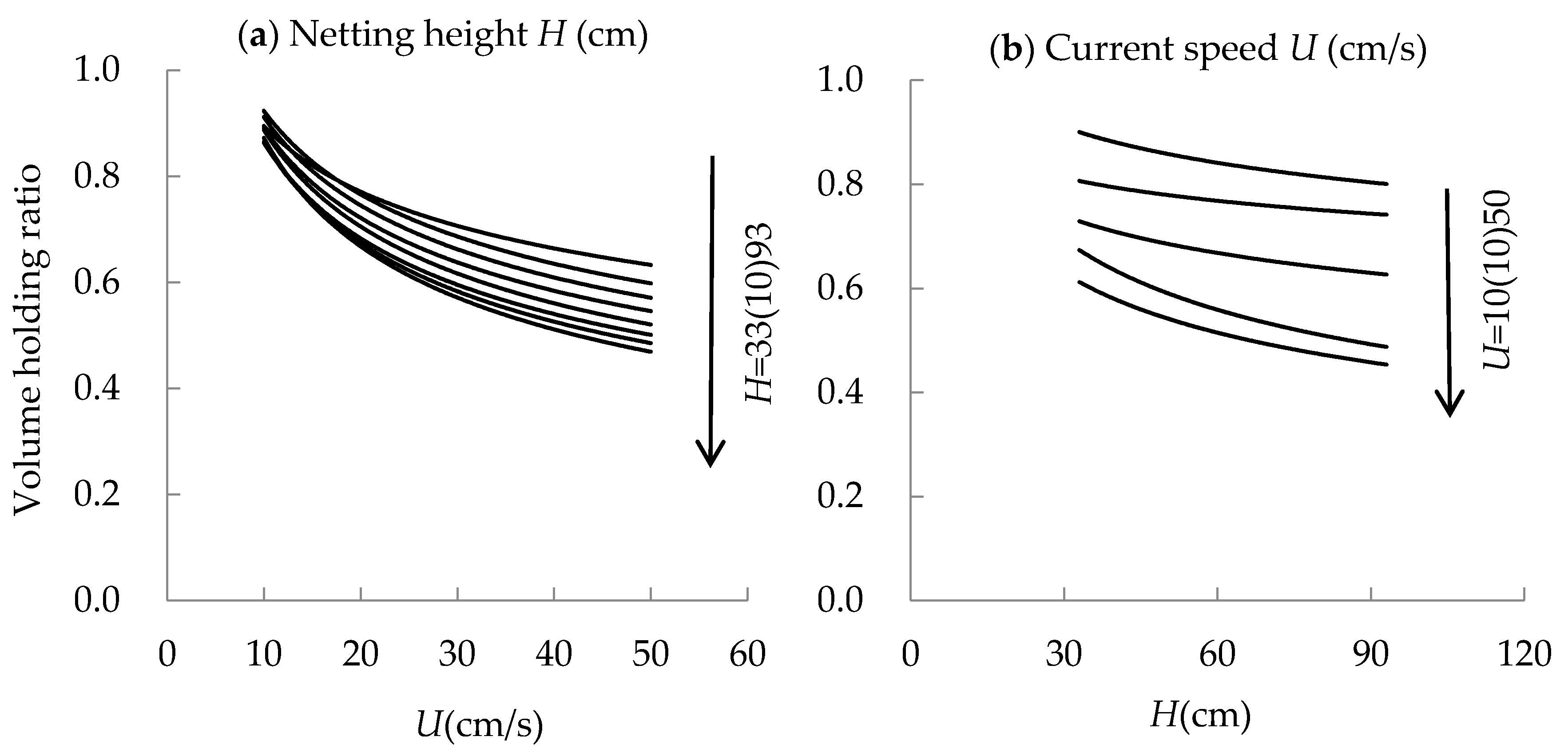
Figure 10.
Relationship of volume holding ratio and net depth plotted against current speed. (a) the relationship of Cv and U for each H; (b) the relationship between Cv and H for each U.
Figure 10.
Relationship of volume holding ratio and net depth plotted against current speed. (a) the relationship of Cv and U for each H; (b) the relationship between Cv and H for each U.
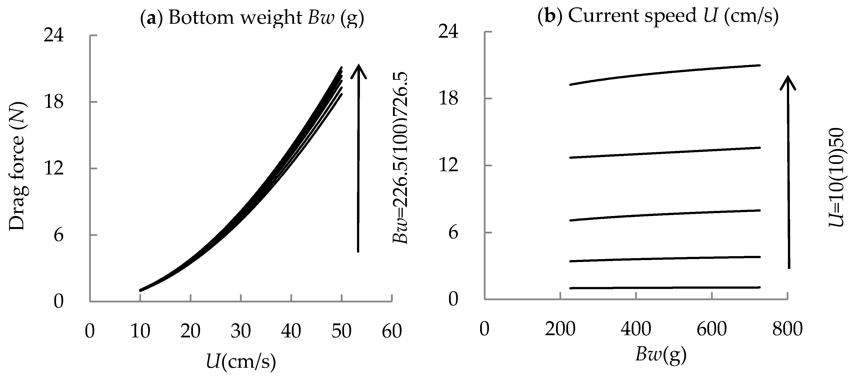
Figure 11.
Relationship of drag force and bottom weight plotted against current speed. (a) the relationship of RD and U for each Bw; (b) the relationship between RD and Bw for each U.
Figure 11.
Relationship of drag force and bottom weight plotted against current speed. (a) the relationship of RD and U for each Bw; (b) the relationship between RD and Bw for each U.
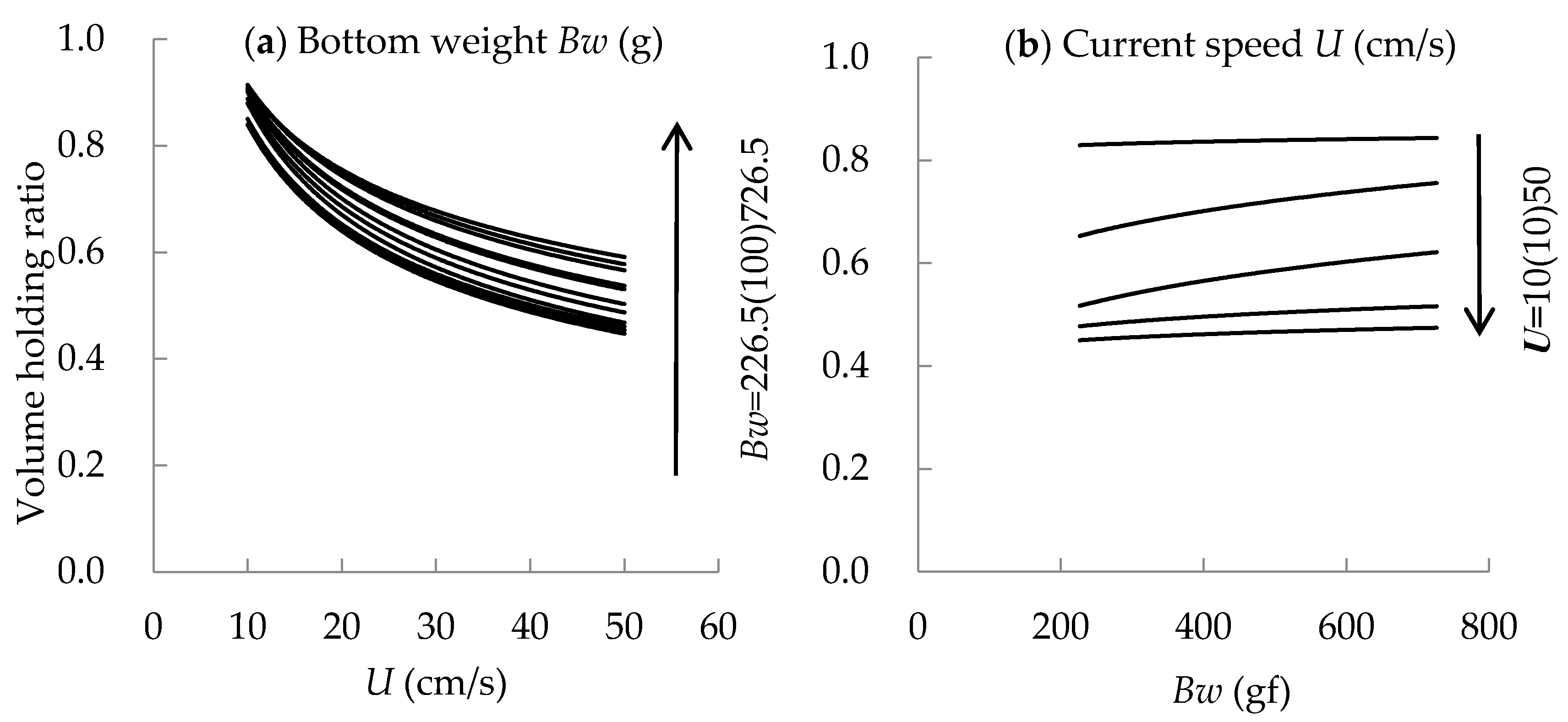
Figure 12.
Relationship of volume holding ratio and bottom weight plotted against current speed. (a) the relationship of Cv and U for each Bw; (b) the relationship between Cv and Bw for each U.
Figure 12.
Relationship of volume holding ratio and bottom weight plotted against current speed. (a) the relationship of Cv and U for each Bw; (b) the relationship between Cv and Bw for each U.
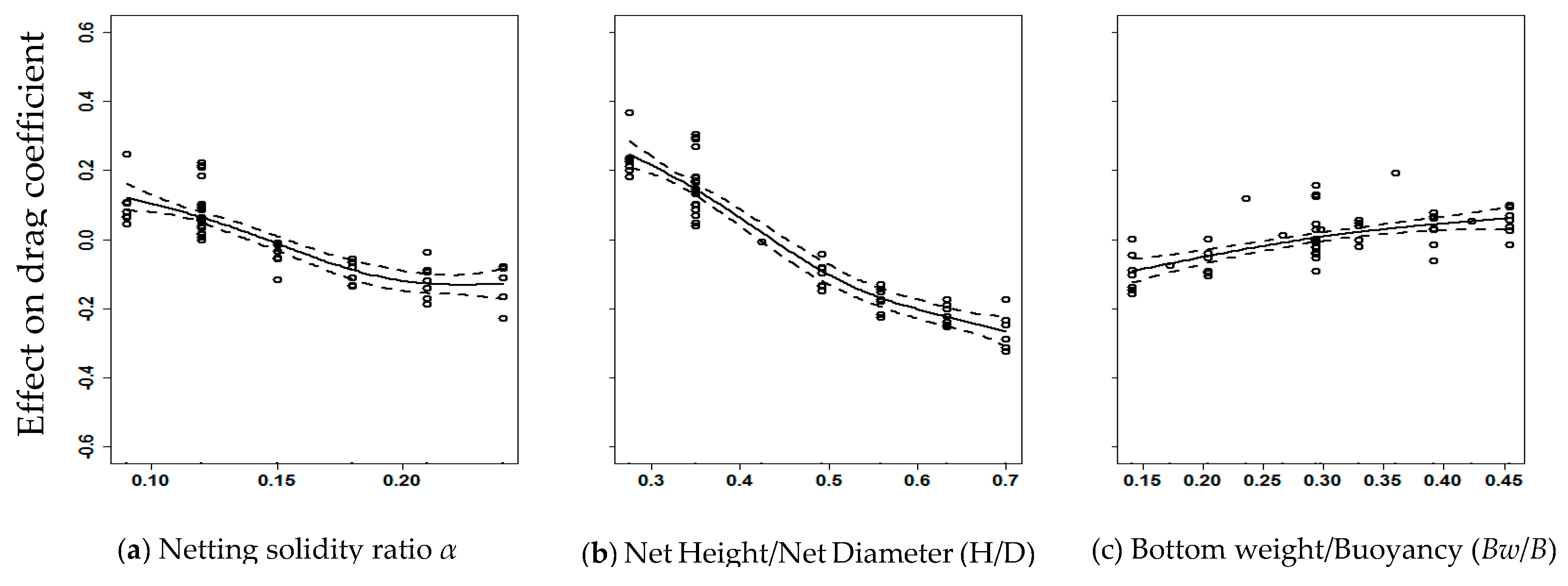
Figure 13.
The relationship between design factors and drag coefficient on the generalized additive (GAM) model. (The y-axis represents the partial effect of each variable; Dashed lines indicate 95% confidence bounds; Solid lines are smooth curves).
Figure 13.
The relationship between design factors and drag coefficient on the generalized additive (GAM) model. (The y-axis represents the partial effect of each variable; Dashed lines indicate 95% confidence bounds; Solid lines are smooth curves).
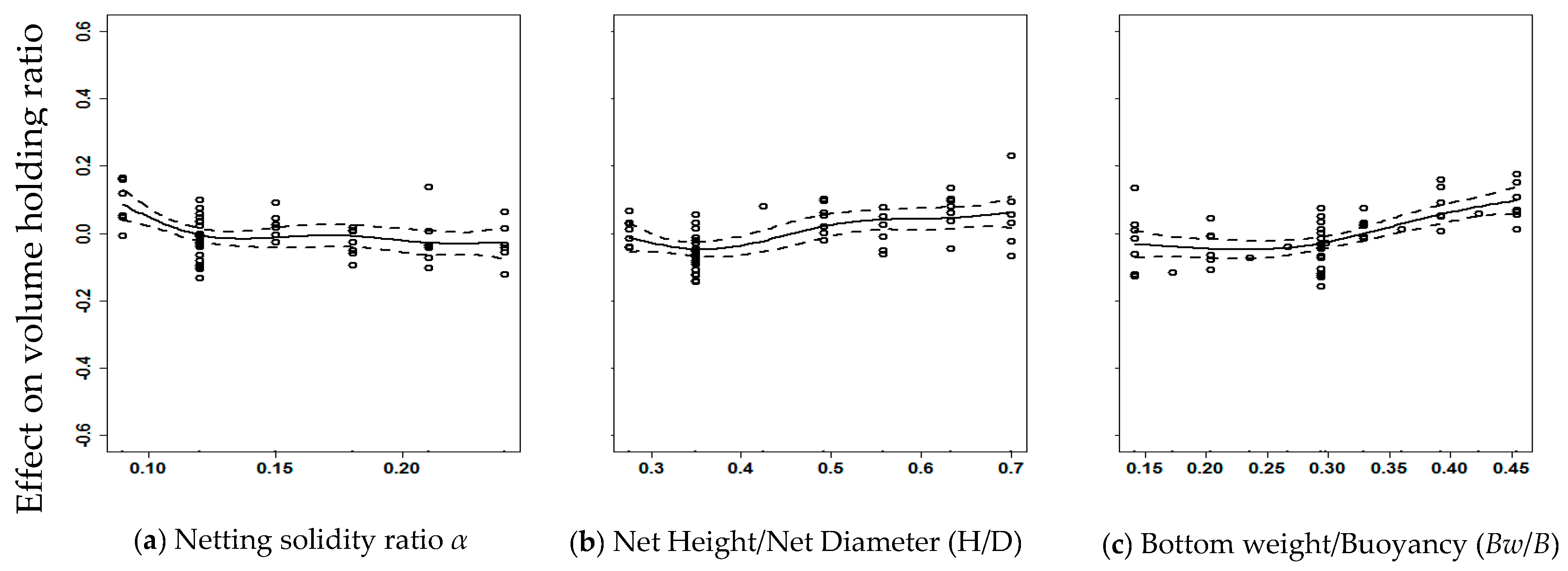
Figure 14.
Relationships between design factors and volume holding ratio in the case of the GAM model. (The y-axis represents the partial effect of each variable; Dashed lines indicate 95% confidence bounds; Solid lines are smooth curves).
Figure 14.
Relationships between design factors and volume holding ratio in the case of the GAM model. (The y-axis represents the partial effect of each variable; Dashed lines indicate 95% confidence bounds; Solid lines are smooth curves).
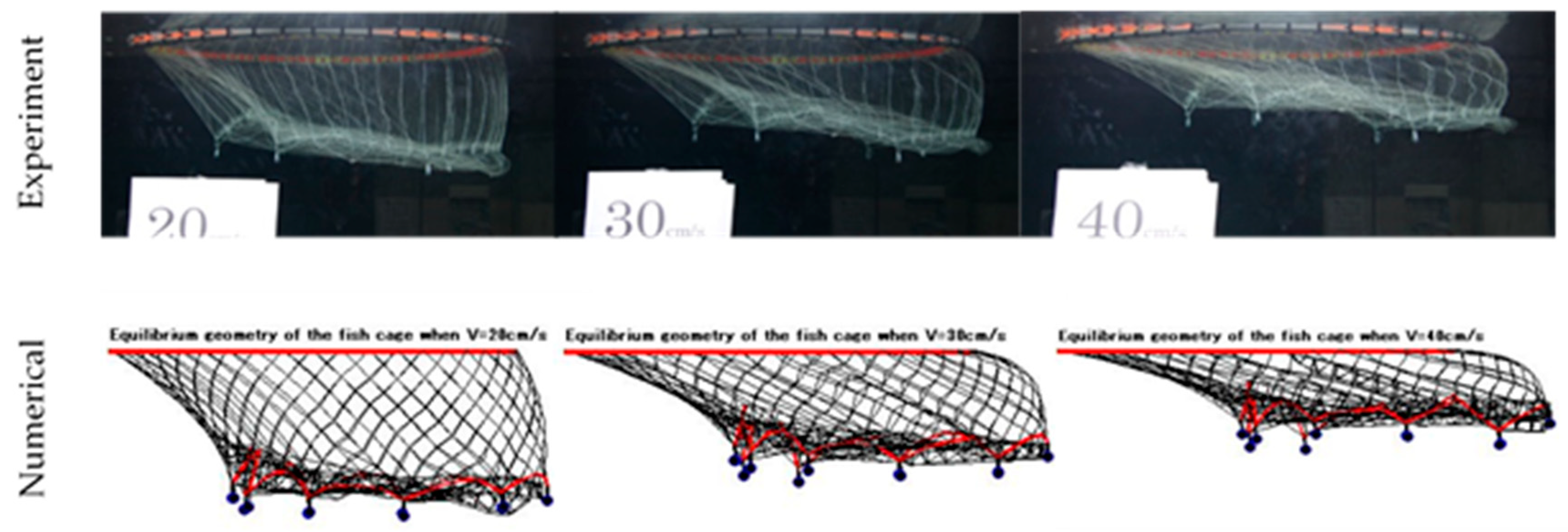
Figure 15.
Snapshots from experimental and numerical simulations.
Figure 15.
Snapshots from experimental and numerical simulations.
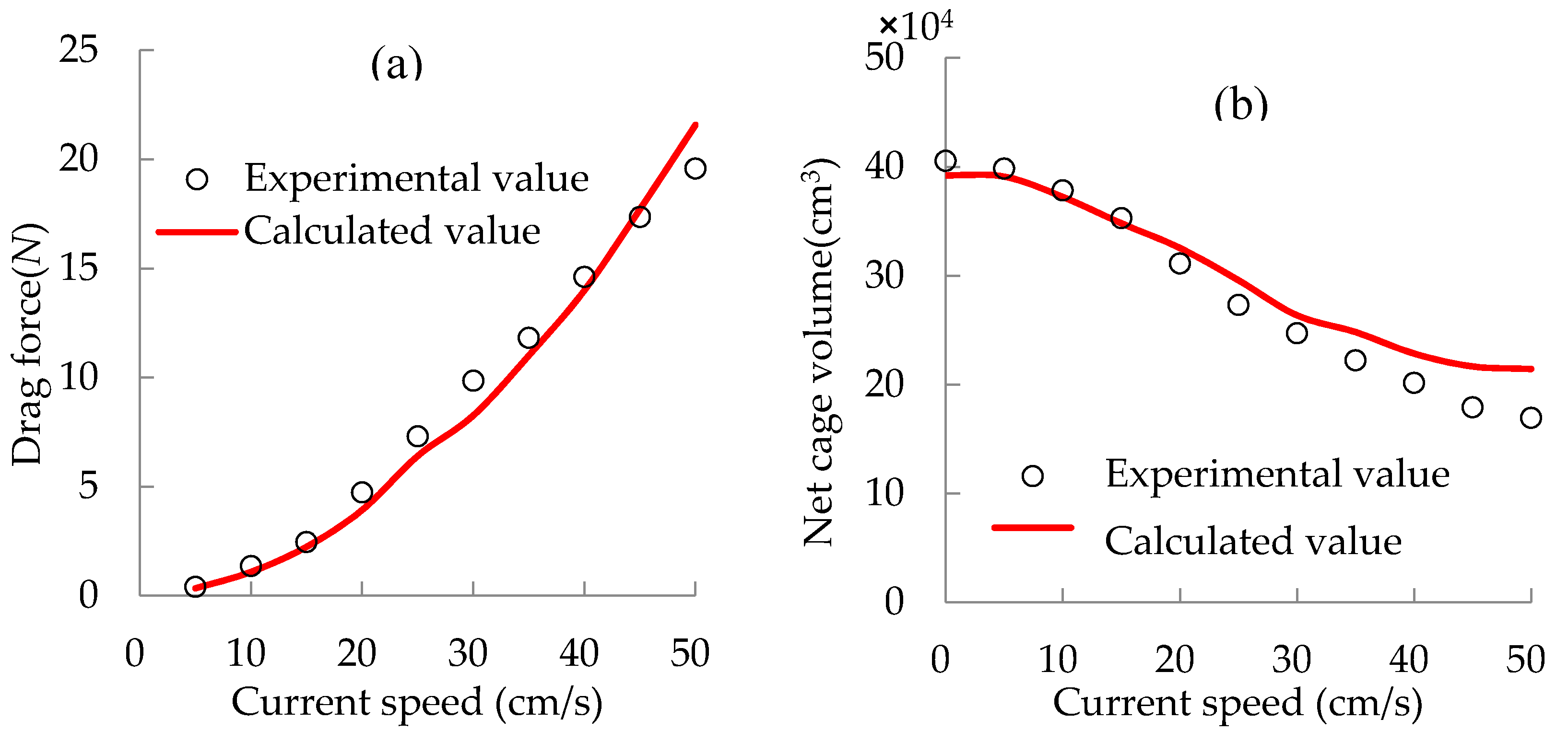
Figure 16.
Comparison of drag force and cage volume between the experimental and simulation results as a function of current speed (α = 0.12, H = 0.42 m, Bw = 476.5 g). (a) the drag force; (b) the cage volume.
Figure 16.
Comparison of drag force and cage volume between the experimental and simulation results as a function of current speed (α = 0.12, H = 0.42 m, Bw = 476.5 g). (a) the drag force; (b) the cage volume.
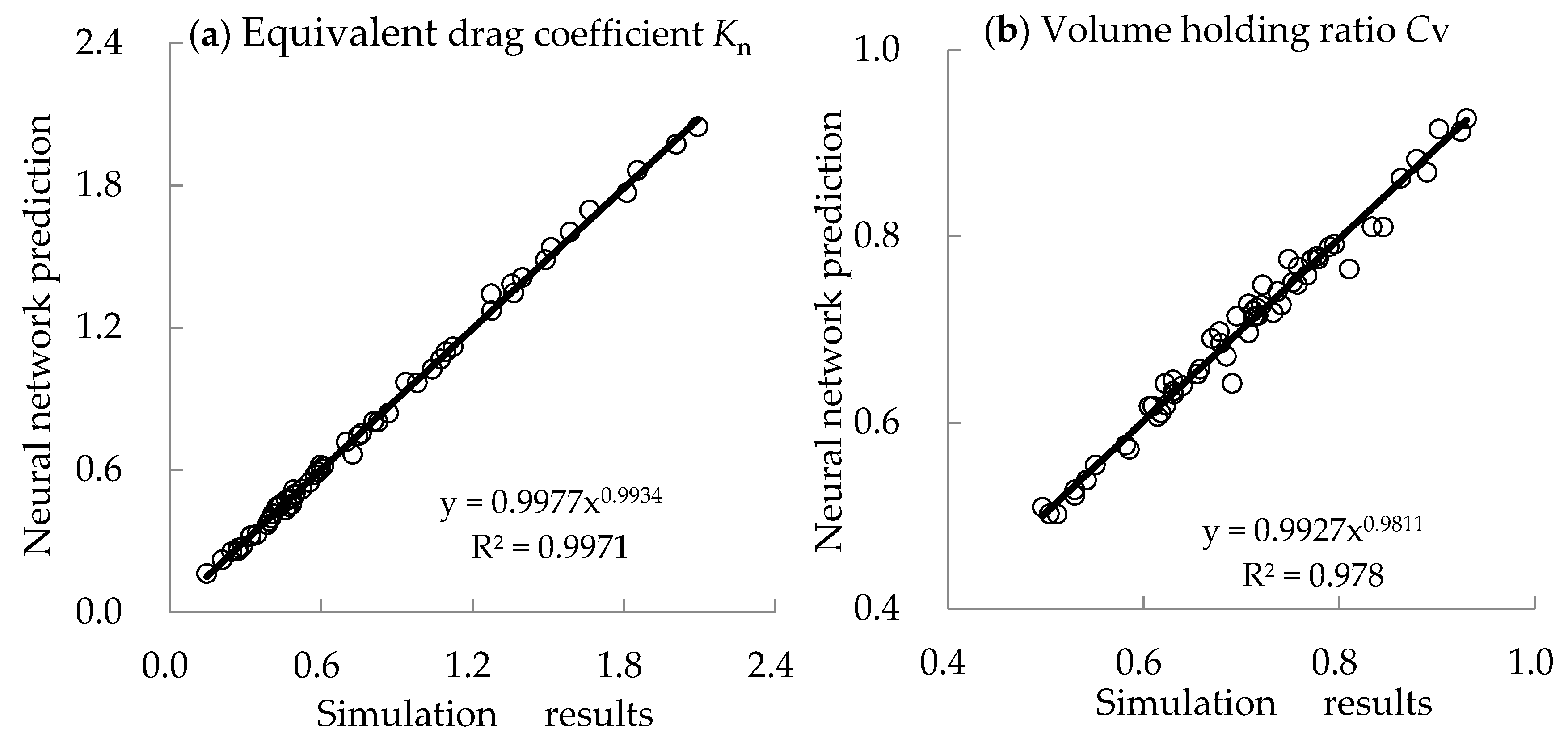
Figure 17.
Relationships between neural network prediction and simulated results. (a) Equivalent drag coefficient; (b) Volume holding ratio
Figure 17.
Relationships between neural network prediction and simulated results. (a) Equivalent drag coefficient; (b) Volume holding ratio
Table 1.
The Specifications of full-scale net cage and model net cage.
Table 1.
The Specifications of full-scale net cage and model net cage.
| Component | Parameter | Prototype Value | Model Value |
|---|
| Floating pipe | Material | High density polyethylene | High density polyethylene |
| General diameter | 34.0 m | 1.2 m |
| Pipe diameter | 35.5 cm | 1.5 cm |
| Side netting | Material | Polyethylene ultra cross knotless netting | Polypropylene knotless |
| Net Height | 12.0 m | 0.42 m |
| Twine diameter | 4.1 mm | 0.6 mm |
| Mesh size | 100.0 mm | 20.0 mm |
| Mesh type | Diamond mesh | Diamond mesh |
| Bottom netting | Material | Polyethylene knotless netting | Polypropylene knotless |
| Twine diameter | 4.1 mm | 0.6 mm |
| Mesh size | 75.0 mm | 20.0 mm |
| Mesh type | Square mesh | Square mesh |
Table 2.
Design parameters of net cage varied in the numerical study.
Table 2.
Design parameters of net cage varied in the numerical study.
| Current Speed U (cm/s) | Netting Solidity α | Netting Height H (m) | Bottom Weights Bw (g) |
|---|
| 10 | 0.06 | 0.33 | 226.5 |
| 20 | 0.09 | 0.42 | 276.5 |
| 30 | 0.12 | 0.51 | 326.5 |
| 40 | 0.15 | 0.59 | 376.5 |
| 50 | 0.18 | 0.67 | 426.5 |
| | 0.21 | 0.76 | 476.5 |
| | 0.24 | 0.84 | 526.5 |
| | 0.27 | 0.93 | 576.5 |
| | 0.3 | | 626.5 |
| | 0.34 | | 676.5 |
| | 0.38 | | 726.5 |
| | 0.42 | | |
| | 0.46 | | |
Table 3.
Statistical results of GAM analysis for volume holding ratio.
Table 3.
Statistical results of GAM analysis for volume holding ratio.
| Model Factors | EDF | F-Value | p-Value |
|---|
| Netting solidity ratio α | 3.32 | 3.68 | 0.008199 |
| Netting height/Diameter of net cage (H/D) | 3.28 | 5.94 | 0.000625 |
| Bottom weight/Buoyancy (Bw/B) | 2.65 | 10.30 | <1.3 × 10⁻⁵ |
Table 4.
Statistical results of GAM analysis for equivalent drag coefficient.
Table 4.
Statistical results of GAM analysis for equivalent drag coefficient.
| Model Factors | EDF | F-Value | p-Value |
|---|
| Netting solidity ratio α | 2.63 | 40.73 | <2.8 × 10⁻¹⁶ |
| Netting height/Diameter of net cage (H/D) | 2.90 | 139.79 | <2.0 × 10⁻¹⁶ |
| Bottom weight/Buoyancy (Bw/B) | 1.71 | 16.00 | <2.7 × 10⁻⁶ |
Table 5.
Weights Wij from the ith input layer to jth hidden layer.
Table 5.
Weights Wij from the ith input layer to jth hidden layer.
| | j | 1 | 2 | 3 | 4 | 5 | 6 | 7 | 8 | 9 | 10 |
|---|
| i | |
|---|
| 1 | 1.970827 | 1.107892 | −1.74519 | 1.920279 | −0.05492 | −2.02666 | −1.56621 | 0.207186 | 2.664381 | 2.094821 |
| 2 | −2.02104 | 1.847165 | 1.984459 | −0.27105 | 2.026001 | −1.78069 | −1.10283 | 2.415709 | 1.12061 | 2.399915 |
| 3 | 1.114336 | −2.07818 | 1.144879 | 2.364004 | 1.274584 | 1.44558 | 2.177577 | −0.59733 | 1.148622 | −1.16935 |
Table 6.
Weights Wjk from the jth hidden layer to kth output layer.
Table 6.
Weights Wjk from the jth hidden layer to kth output layer.
| | j | 1 | 2 | 3 | 4 | 5 | 6 | 7 | 8 | 9 | 10 |
|---|
| k | |
|---|
| 1 | −0.5315 | 0.275588 | −0.12305 | −0.04154 | 0.305313 | −0.41142 | 1.005371 | −0.83501 | −0.32428 | 0.95714 |
| 2 | 0.06715 | −0.18221 | −0.00363 | −0.02391 | −0.19082 | 0.163327 | −0.00961 | −0.04366 | −0.00862 | −0.44308 |


