An Effective Multiscale Methodology for the Analysis of Marine Flexible Risers

Abstract

Life extension is an attractive option for subsea flexible risers nearing the end of their design lives. However, techniques for assessing accumulated fatigue damage in flexible risers are often associated with large uncertainties due to the simplified calculation approaches typically used. One approach to reducing uncertainties is the inclusion of nonlinearities in riser structural response and consistent linking between global and local models. In this article, we present the elements of a numerical multiscale procedure capable of predicting the stresses that lead to fatigue damage in flexible pipes, namely: a nonlinear beam element, a nonlinear section response model and a detailed finite element model; the consistent integration of models developed for different length scales; and finally a validation of the flexible riser large-scale model.

1. Introduction

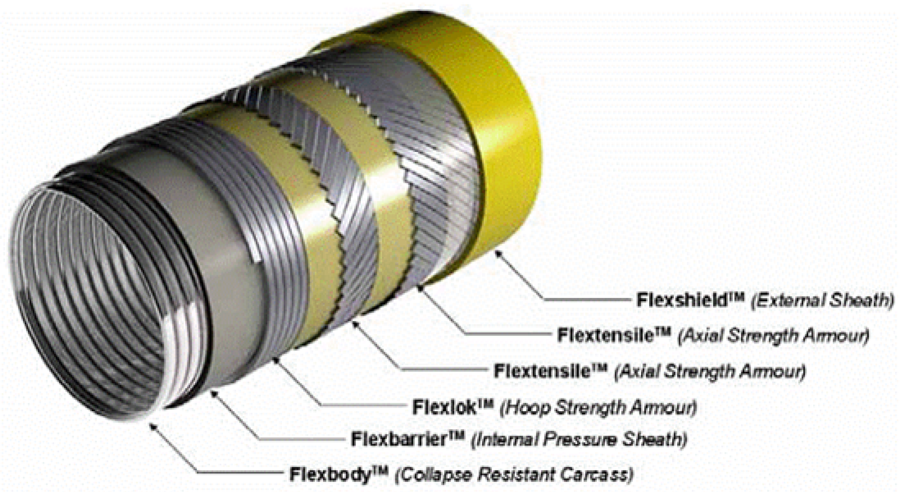
Since their introduction in the 1970s, unbonded flexible risers have proved an effective and reliable solution for the transfer of fluids in the offshore environment. In contrast to steel risers, flexible risers are able to deform and reposition in response to external loading without incurring damage [1,2]. This flexibility is a consequence of the structure of flexible pipes, which includes multiple layers consisting of wound steel profiles and extruded polymers (Figure 1). However, the current trend towards production in deeper waters have led to new failure modes arising, such as buckling of helical wires, threatening long-term integrity. These failure modes are often progressive in nature and challenging to predict [1]. In addition, accurate determination of the fatigue damage is necessary to ensure that life prediction of ageing flexible risers can be made with confidence.

In distinction to bonded risers using composite materials, for which finite-element based structural analysis has been demonstrated by Sun et al. [3], Amaechi et al. [4], among others, the analysis of unbonded flexible risers presents unique challenges as their performance relies on the ability of internal components to slide relative to each other (constrained by geometry and friction) to relieve load. Nevertheless, the multiscale methods presented in this article are also applicable to the analysis of bonded composite risers.

In the following, we describe models and processes used in a numerical multiscale procedure for the analysis of flexible pipes/risers. In this procedure, local and global models are integrated in order to obtain greater accuracy. Two versions of this integration have been developed, a fully-integrated procedure and a sequentially-integrated procedure. Firstly, we present a local finite element (FE) model and show results for various elementary loadings. Secondly, we describe a section response model that aims to capture the nonlinear relationship between stress resultants and section deformation measures noted in flexible pipes. This model is then calibrated using simulation results from the FE model. Thirdly, procedures for combining these models in multiscale analysis are described. A simplified demonstration of the integrated multiscale procedure and validation of the global analysis model are shown.

A beam element formulation for the global dynamical analysis of flexible risers was earlier presented by McNamara et al. [5], who introduced the mixed formulation adopted in the current work. Yazdchi and Crisfield [6] describe a 2D corotational beam element for representing flexible risers including shear deformations and the derivation of load stiffness matrices. Higher order effects such as the influence of curvature on buoyancy are included. Related work by the same authors [7] extends this approach for 3D elements and loading. A detailed formulation for flexible polymer hoses used as used in the drilling industry is presented by Monprapussorn et al. [8]. This treatment includes large deformations, coupled radial-axial deformations and, in addition, interactions between both of these effects with the internal flow. This work, despite providing a thorough treatment of internal flow effects, is less relevant for unbonded flexible risers used in production, as pipe walls cannot be represented as thin-walled pipes with linear elastic behaviour.

Several software packages have been developed for global dynamic analysis of flexible risers. The underlying numerical approaches used in these packages include both classical finite element methods and lumped-mass and -stiffness approaches. Packages available commercially include Orcaflex, Flexcom, Riflex and Deepflex. Local analysis tools for flexible pipes include purely analytical formulations, finite element models and analytical formulations solved by numerical means. One significant challenge in local analysis is the accurate calculation of the displacement of the initially helical armours as the pipe bends. Additionally, the use of unrealistic boundary conditions at the end sections of the model can lead to inaccuracies in the solution. Earlier local models focussed on analytical approaches, including the derivation of linear stiffness matrices (for example, by McNamara and Harte [9]) and analyses of pipe bending and associated wire slippage [10,11]. Tan et al. [12] have shown using finite element investigations that the kinematics of tensile armour wires is complex and depends of a number of geometric parameters. An example of a detailed finite element model for flexible pipe is given by Leroy and Estrier [13], in which contact is computed between all layers. In this model periodic boundary conditions are used to constrain relative motions at the ends of tensile wires, allowing a shorter model to predict tensile wire stresses accurately. Finite element models have also been developed by Sousa et al. [14], who provide an analytical derivation for the properties of an orthotropic stiffness layer used as a simplification of the carcass layer and a physical basis for the penalty stiffness used to compute layer interactions. This model is employed to investigate the load redisctibution effects that occur after tensile wire failure. An alternative finite-element based approach has been developed by Sævik and co-workers [15], in which novel finite elements are used to discretise tensile wires and their interactions. This model has subsequently been commercialised in the package BFLEX. An analytical-numerical approach is described by Østergaard et al. [16], based on a formulation of wire kinematics and dynamics resulting in six coupled differential equations, which are solved numerically.

Approaches for combining local and global models include methodologies developed by Caleyron et al. [17], who combine instances of a short finite element model with a virtual spine formed with kinematic constraints to represent a section of flexible riser under a bend stiffener. The application of global loads (tension, constant curvature and torsion) to the spine governs the loading on the component local models. An alternative approach is shown by Majed et al. [18], in which modal superposition-type approaches are used to reduce the computational effort required for a detailed finite element model. This approach requires bending-moment curvature data to be provided so that nonlinearity in pipe response can be incorporated. Earlier development on the multiscale methodology presented in the current work was detailed by Edmans et al. [19,20,21,22].

Analysis problems where features of geometry, physical phenomena and mechanisms and/or behaviour of interest are described or defined at different scales arise frequently in solid and structural mechanics. In the field of composite materials, computational homogenisation has been proposed as a numerical method for handling such situations [23,24]. In this approach, a detailed characterisation of the small-scale structure is created that is large enough to be representative of the structure’s geometry and capture all relevant phenomena. The solution procedure then uses a homogenised large-scale representation within which the detailed representation acts as the constitutive model (for an example, see Geers et al. [25]). The procedure allows for different modelling approaches (e.g., element choice), numerical schemes and incrementation to be used for the component models, increasing computational efficiency. The work of Sacco [26] serves as an example of the broad scope of this technique, where the application of a variant of this technique to investigate crack growth in masonry walls is described.

2. Global Riser Representation

In this section, a two-noded co-rotational Hybrid Beam Element (HBE) is developed to enable implicit dynamic analysis of flexible risers, based on the co-rotational formulations presented by Battini, Crisfield and Le [27,28,29]. The HBE employed in this present research is used to overcome the difficulty resulting from the relative inextensibility of the flexible riser, which leads to an ill-conditioned global tangent stiffness matrix causing convergence issues [5]. The proposed HBE is formulated such that it can incorporate the plastic constitutive model described in Section 3. It is implemented as a “User Element Subroutine” in the commercial FEA software package Abaqus, enabling the static and dynamic analysis of a flexible riser to be solved using the implicit formulation in Abaqus/Standard.

2.1. Kinematics

In the global Cartesian coordinate system, the degrees of freedom (DOFs) of a material point of the proposed HBE element include three translational and three rotational DOFs. Following corotational frameworks described in the literature [27,28,29] (Figure 2), a co-rotational local coordinate system is defined in order to remove the rigid body rotations.

In Figure 2, the local coordinate system follows the orientation of the element in the current configuration, represented by the orthogonal orientation matrix $\mathit{O}=\left[\begin{array}{ccc}{\mathit{r}}_1& {\mathit{r}}_2& {\mathit{r}}_3\end{array}\right]$. The basis vectors ${\mathit{r}}_i$ define the current beam orientation, where ${\mathit{r}}_1$ is the beam axial vector, with direction from the first to the second node. $\mathit{O}$ defines the orientation of the global basis vectors with respect to the current beam local basis vectors. Similarly, the initial local reference system is defined by an orthogonal matrix ${}^0\mathit{O}=\left[\begin{array}{ccc}{}^0{\mathit{r}}_1& {}^0{\mathit{r}}_2& {}^0{\mathit{r}}_3\end{array}\right]$. The initial nodal triads of two end nodes that define the nodal orientations are denoted by ${}^0{\mathit{T}}^1=\left[\begin{array}{ccc}{}^0{\mathit{t}}_1^1& {}^0{\mathit{t}}_2^1& {}^0{\mathit{t}}_3^1\end{array}\right]$ and ${}^0{\mathit{T}}^2=\left[\begin{array}{ccc}{}^0{\mathit{t}}_1^2& {}^0{\mathit{t}}_2^2& {}^0{\mathit{t}}_3^2\end{array}\right]$ A left superscript 0 is used for symbols representing quantities in the initial configuration, otherwise the current configuration is implied, whereas right superscripts for matrices indicates the local node number. A right superscript g is used to indicate global quantities, otherwise a local quantity is implied. If the initial configuration of the beam is straight, the nodal basis vectors coincide with the element basis vectors. The orthogonal rotation matrices ${\mathit{R}}^i$ represent a rotation of the initial nodal triads ${}^0{\mathit{T}}^1$ and ${}^0{\mathit{T}}^2$ to the nodal triads ${\mathit{T}}^1=\left[\begin{array}{ccc}{\mathit{t}}_1^1& {\mathit{t}}_2^1& {\mathit{t}}_3^1\end{array}\right]$ and ${\mathit{T}}^2=\left[\begin{array}{ccc}{\mathit{t}}_1^2& {\mathit{t}}_2^2& {\mathit{t}}_3^2\end{array}\right]$ in the current configuration. In the absence of nodal rotations in the current configuration, ${\mathit{t}}_1^1$, ${\mathit{t}}_1^2$ and ${\mathit{r}}_1$ are collinear. The orthogonal rotation matrices ${\mathit{R}}^1$ and ${\mathit{R}}^2$ define the local rotations at nodes relative to the element basis vectors in the current configuration. The degrees of freedom of the element in global coordinates at time n can be collected as

$$\begin{array}{cc}\hfill {\mathit{d}}^g& ={\left({\mathit{u}}_1^{gT},{\mathit{\theta }}_1^{gT},{\mathit{u}}_2^{gT},{\mathit{\theta }}_2^{gT},N\right)}^T\hfill \\ \hfill & ={\left(u_{11}^g,u_{12}^g,u_{13}^g,{\theta }_{11}^g,{\theta }_{12}^g,{\theta }_{13}^g{u}_{21}^g,u_{22}^g,u_{23}^g,{\theta }_{21}^g,{\theta }_{22}^g,{\theta }_{23}^g,N\right)}^T\hfill \end{array}$$

(1)

Here, ${\mathit{u}}_1^g$ and ${\mathit{u}}_2^g$ denote the global translational DOFs at the two nodes with components $u_{ij}^g$, where i and j represent the node and component indices, respectively. Similarly, ${\mathit{\theta }}_1^g$ and ${\mathit{\theta }}_2^g$ denote the global rotational DOFs with components ${\theta }_{ij}^g$. The inclusion of the beam axial force N in the element DOF vector results from the use of the mixed formulation developed by McNamara et al. [5] to handle the high axial stiffness of flexible pipes effectively, in which the element axial force appears as a Lagrange multiplier enforcing an inextensibility constraint. Local displacements and rotations for the HBE are defined with reference to the directions defined by the element triad $\mathit{O}$, and denoted with

$$\begin{array}{cc}\hfill \mathit{d}& ={\left(u,{\mathit{\theta }}_1^T,{\mathit{\theta }}_2^T,N\right)}^T\hfill \\ \hfill & ={\left(u,{\theta }_{11}^{},{\theta }_{12}^{},{\theta }_{13}^{},{\theta }_{21}^{},{\theta }_{22}^{},{\theta }_{23}^{},N\right)}^T\hfill \end{array}$$

(2)

where u denotes the axial displacement, and ${\mathit{\theta }}_1$ and ${\mathit{\theta }}_2$ denote the local rotations at the two nodes with components ${\theta }_{ij}$. The axial force term N is identical to the global term in Equation (1). Full definitions of the local quantities u, ${\mathit{\theta }}_1$ and ${\mathit{\theta }}_2$ are given by Battini [27] and Crisfield [28]; here, it suffices to note that the calculation of these local quantities is such that the local translational displacement at the first node is always zero. Local nodal rotations are calculated by effectively subtracting the nodal rotations associated with the element reference frame. The finite rotation is described by additive rotational vectors based on the parameterization of finite rotations [27,28].

The orientation of the local frame in the initial configuration can be determined from its geometry as

$$\begin{array}{cc}\hfill {}^0{\mathit{r}}_1& =\left({}^0{\mathit{x}}_2-{}^0{\mathit{x}}_1\right)/l_0\hfill \end{array}$$

(3)

$$\begin{array}{cc}\hfill {}^0{\mathit{r}}_3& =\frac{{}^0{\mathit{r}}_1\times {\mathit{e}}_2}{∥{}^0{\mathit{r}}_1\times {\mathit{e}}_2∥}\hfill \end{array}$$

(4)

$$\begin{array}{cc}\hfill {}^0{\mathit{r}}_2& ={}^0{\mathit{r}}_3\times {}^0{\mathit{r}}_1\hfill \end{array}$$

(5)

where $l_0$ is the element length in the initial configuration. If ${}^0{\mathit{r}}_1={\mathit{e}}_2$ or ${}^0{\mathit{r}}_1=-{\mathit{e}}_2$, then the alternative definition ${}^0{\mathit{r}}_3={\mathit{e}}_3$ and ${}^0{\mathit{r}}_2={}^0{\mathit{r}}_3\times {}^0{\mathit{r}}_1$ are used.

Given the global DOF solutions ${\mathit{d}}^g=\left({\mathit{u}}_1^g{\mathit{\theta }}_1^{gT}{\mathit{u}}_2^g{\mathit{\theta }}_2^{gT}N\right)$ the nodal triads can then be updated by rotating the initial triads to the current triads using the rotation matrix ${\mathit{R}}^i$ (following Crisfield [28]):

$$\begin{array}{c}\hfill {\mathit{T}}^1=\left({\mathit{R}}^1\right){}^0{\mathit{T}}^1,{\mathit{T}}_2=\left({\mathit{R}}^2\right){}^0{\mathit{T}}^2\end{array}$$

(6)

where ${\mathit{R}}^i\left({\mathit{\theta }}^{ig}\right)$ is computed from the global nodal rotations using the Rodrigues formula [28]. For a consistent definition of beam local displacements and curvatures, the vector representing the beam transverse axis $\mathit{p}$ must be rotated consistently with the element rotation. To this end, the global basis vector ${\mathit{e}}_2$ is rotated first into the initial configuration and then to the current configuration for each node, that is, ${\mathit{p}}^i=\left({\mathit{R}}^i\right)\left({}^0\mathit{O}\right){\mathit{e}}_2$. A sufficiently accurate approximation $\mathit{p}$ can be obtained from the arithmetic mean of the two vectors ${\mathit{p}}^1$ and ${\mathit{p}}^2$. This allows the three direction vectors of the current element triads, ${\mathit{r}}_1$, ${\mathit{r}}_2$ and ${\mathit{r}}_3$ to be obtained:

$$\begin{array}{cc}\hfill {\mathit{r}}_1& =\left({\mathit{x}}_2^g-{\mathit{x}}_1^g\right)/l\hfill \end{array}$$

(7)

$$\begin{array}{cc}\hfill {\mathit{r}}_3& =\frac{{\mathit{r}}_1\times \mathit{p}}{∥{\mathit{r}}_1\times \mathit{p}∥}\hfill \end{array}$$

(8)

$$\begin{array}{cc}\hfill {\mathit{r}}_2& ={\mathit{r}}_3\times {\mathit{r}}_1\hfill \end{array}$$

(9)

where l is the element length in the current configuration. These vectors are collected to define the element rotation matrix $\mathit{R}$. The use of $\mathit{p}$ rather than ${\mathit{e}}_2$ avoids sign change problems for local quantities if the the angle between the beam axis and ${\mathit{e}}_2$ becomes small. Collecting these three vectors into a matrix $\mathit{O}$ forms the element rotation matrix in the current configuration, which is used in the computation of local degrees of freedom.

The nodal rotation vectors, defined relative to the current element frame, can then be found by rotating the initial local element frame to the current nodal local frame and then rotating back to the current local element frame [27].

$$\begin{array}{c}\hfill {\mathit{\theta }}^i=log\left({\overline{\mathit{R}}}^i\right),{\overline{\mathit{R}}}^i={\mathit{R}}^T\left({\mathit{R}}^i\right)\mathit{O}\end{array}$$

(10)

2.2. Variational Formulation

Equilibrium conditions for the HBE are developed using a variational formulation, which is augmented to impose an inextensibility condition. The augmented virtual internal virtual work is thus

$$\begin{array}{c}\hfill \delta W^{int}={\int }_0^l\left[N\delta \epsilon +M_1\delta {\kappa }_1+M_2\delta {\kappa }_2+M_3\delta {\kappa }_3+\left(\epsilon -\frac{N}{EA}\right)\delta N\right]\mathrm{d}l\end{array}$$

(11)

The full derivation for Equation (11) is provided by McNamara et al. [5]. The stress resultants N are M are calculated using the nonlinear constitutive model developed in Section 3 and local deformation measures.

2.3. Discretization and Integration

Standard shape functions based on beam local coordinates are used to calculate generalised strain.A three-point Gauss integration scheme is adopted in order to allow curvature variation to be captured within a single element and allowing longer elements to be used. A linear shape function is used to interpolate the axial deformation:

$$\begin{array}{c}\hfill u\left(\xi \right)=\frac{1}{2}\left(1+\xi \right)u\end{array}$$

(12)

Cubic Hermite shape functions are used to interpolate local transverse displacements. Local displacements are computed such that the transverse local displacements at the two end nodes are zero [28]. The shape functions are then given as

$$\begin{array}{cccc}\hfill w_i& =\frac{l}{8}{\left[\begin{array}{c}({\xi }^2-1)(\xi -1)\\ ({\xi }^2-1)(\xi +1)\end{array}\right]}^T\left[\begin{array}{c}{\theta }_{1i}\\ {\theta }_{2i}\end{array}\right]\hfill & \hfill i& =1,2,3\hfill \end{array}$$

The local section rotation along the beam is found from the derivatives of the transverse displacements as

$$\begin{array}{c}\hfill {\theta }_i=\frac{1}{4}{\left[\begin{array}{c}3{\xi }^2-2\xi -1\\ 3{\xi }^2+2\xi -1\end{array}\right]}^T\left[\begin{array}{c}{\theta }_{1i}\\ {\theta }_{2i}\end{array}\right]\end{array}$$

(13)

Further differentiation provides the curvature along the beam as

$$\begin{array}{cc}\hfill {\kappa }_i& =\frac{1}{l}{\left[\begin{array}{c}-1+3\xi \\ 1+3\xi \end{array}\right]}^T\left[\begin{array}{c}{\theta }_{1i}\\ {\theta }_{2i}\end{array}\right]=\left[\begin{array}{cc}{B}_1& B_2\end{array}\right]\left[\begin{array}{c}{\theta }_{1i}\\ {\theta }_{2i}\end{array}\right]\hfill \end{array}$$

In the following development, the subscript l will be used to denote quantities and operators defined in the corotational frame while the subscript g will be used for quantities transformed for assembly in system global matrices. The generalized strains ${\mathit{\epsilon }}_l$ can thus be computed along the beam in the local coordinates

$$\begin{array}{cc}\hfill {\mathit{\epsilon }}_l& ={\left(\begin{array}{ccccc}u/l& {\kappa }_1& {\kappa }_2& {\kappa }_3& N\end{array}\right)}^T={\mathit{B}}_l\mathit{d}\hfill \end{array}$$

(14)

where, ${\mathit{B}}_l$ is the displacement-strain matrix in the following form

$$\begin{array}{c}\hfill {\mathit{B}}_l=\left[\begin{array}{cccccccc}\frac{1}{l}& 0& 0& 0& 0& 0& 0& 0\\ 0& B_1& 0& 0& B_2& 0& 0& 0\\ 0& 0& B_1& 0& 0& B_2& 0& 0\\ 0& 0& 0& B_1& 0& 0& B_2& 0\\ 0& 0& 0& 0& 0& 0& 0& 1\end{array}\right]\end{array}$$

(15)

Once the generalized strains are found, the internal force vector ${\mathit{f}}_l$ and tangent stiffness matrix ${\mathit{K}}_l$ can then be calculated in local coordinates:

$$\begin{array}{cc}\hfill {\mathit{f}}_l& ={\int }_l{\mathit{B}}_l^T{\mathit{\sigma }}_l\left({\mathit{\epsilon }}_l\right)\mathrm{d}l\hfill \end{array}$$

(16)

$$\begin{array}{cc}\hfill {\mathit{K}}_l& ={\int }_l{\mathit{B}}_l^T{\mathit{D}}_l{\mathit{B}}_l\mathrm{d}l\hfill \end{array}$$

(17)

The material tangent matrix ${\mathit{D}}_l$ and the generalized stress ${\mathit{\sigma }}_l\left({\mathit{\epsilon }}_l\right)$ are provided by the constitutive models developed in Section 3). The material tangent matrix ${\mathit{D}}_l$ is

$$\begin{array}{c}\hfill \mathit{D}=\left[\begin{array}{lllll}0& 0& 0& 0& 1\\ 0\hfill & GJ& 0& 0& 0\\ 0\hfill & 0& D_{33}& D_{34}& 0\\ 0\hfill & 0& D_{43}& D_{44}& 0\\ 1\hfill & 0& 0& 0& -\frac{1}{EA}\end{array}\right]\end{array}$$

(18)

The entries $GJ$, $EA$, $D_{33}$, $D_{34}$, $D_{43}$, $D_{44}$ of the matrix $\mathit{D}$ are calculated by the elastoplastic constitutive model presented in Section 3. The internal force vector ${\mathit{f}}_g$ and tangent stiffness ${\mathit{K}}_g$ can then be calculated in global coordinates by applying the coordinate transformation as follows:

$$\begin{array}{cc}\hfill {\mathit{f}}_g& ={\mathit{B}}_{trans}^T{\mathit{f}}_l\hfill \end{array}$$

(19)

$$\begin{array}{cc}\hfill {\mathit{K}}_g& ={\mathit{B}}_{trans}^T{\mathit{K}}_l{\mathit{B}}_{trans}\hfill \end{array}$$

(20)

The derivation of the coordinate transformation matrix ${\mathit{B}}_{trans}^{}$ is described by Battini [27].

For this work, the calculations of ${\mathit{f}}_g$ and ${\mathit{K}}_g$ in each element are implemented in a user element subroutine for Abaqus.

2.4. Execution

A mass matrix is included in the HBE implementation. In the current work, only the translational inertia effect is considered, as suggested by Crisfield [28]. The HBE is designed to work with the Abaqus solver by returning the element residual vector and tangent stiffness matrix (in global coordinates) at every iteration. Time integration is handled by Abaqus using the Hilber-Hughes-Taylor (HHT) method [30].

3. Section Response Modelling

In this section, a semi-empirical nonlinear constitutive model is developed to relate section resultants to section deformation measures in the proposed hybrid beam element.

3.1. Elastic Modelling

We consider a representative volume element (RVE) of the flexible riser - a hollow tube with internal and external radii a and $b,$ and the center-line length $\ell .$ As shown in Figure 3, the representative hollow tube is subjected to bending moments $M_1$ and $M_2,$ twisting moment $M_3,$ and axial force $N,$ as well as internal and external pressure $p_i$ and $p_e$. Its local state is described by curvature of the center-line, ${\kappa }_1$ and ${\kappa }_2,$ torsion ${\kappa }_3$, and axial strain $\epsilon$.

As described in Section 1, flexible pipes are multilayer composite periodic structures. Accordingly, we propose the following linear elastic constitutive relations as representative for small displacements and curvatures for the Euler-Bernoulli beam (Figure 3):

$$\begin{array}{cccc}\hfill {\kappa }_1& =\frac{M_1}{E_{b}I}\hfill & \hfill {\kappa }_2& =\frac{M_2}{E_{b}I}\hfill \\ \hfill {\kappa }_3& =\frac{M_3-M_3^0}{G_{t}J}\hfill & \hfill \epsilon & =\frac{N-N_0}{E_e{A}_m}\hfill \end{array}$$

(21)

In the above $I=\frac{1}{4}\pi \left(b^4-a^4\right)$ and $J=\frac{1}{2}\pi \left(b^4-a^4\right)$ are bending and torsional second moments of area, and $A_m=\pi \left(b^2-a^2\right)$ is the cross-sectional area of the pipe excluding the bore. Due to the anisotropy of the pipe, we assume that $E_b,$ $G_t$ and $E_e$ are independent elastic (Young’s or shear) moduli for bending, torsion and extension. As shown later, these moduli are pressure-dependent and can be calibrated for different pressure levels. $M_3^0$ and $N_0$ are the initial torque and axial force induced by internal and external pressures under fixed torsional and extensional constraints, respectively.

Consistent with the available local degrees of freedom defined for the beam element in Section 2, the continuum kinematic definitions of the generalised strains read

$$\begin{array}{cccc}\hfill {\kappa }_i& =\frac{d{\theta }_i}{dl},i=1,2,3 \hfill & \hfill \epsilon & =\frac{du}{dl}\hfill \end{array}$$

(22)

3.2. Vector Hysteresis Model

As the flexural structure response of risers exhibits a hysteretic behavior, the bending moment is not a single-valued function of curvature. As a result, cyclic bending is associated with deformations that are not immediately recovered on unloading. To determine the bending moment in a single-valued manner, we should enlarge the state space (of thermodynamics) by introducing internal variables to describe the sliding-induced irreversible curvatures. Due to the nature of the physical mechanisms acting on the layers, such internal variables are much l ike plastic strains in conventional plasticity.

We borrow some concepts from plasticity in developing a hysteresis model for flexible risers. The sliding-induced irreversible curvature can be taken as the accumulated plastic strain in conventional plasticity. Both are loading history dependent internal variables.

In light of the mechanical representation of bending-induced hysteresis, we introduce a pair of work-conjugate 4-component vectors, $\mathit{M}$ and $\kappa$ defined as

$$\begin{array}{cccc}\hfill \mathit{M}& =\left(\begin{array}{c}\hfill M_1\\ \hfill M_2\\ \hfill \alpha \left(M_3-M_3^0\right)\\ \hfill \beta \ell \left(N-N_0\right)\end{array}\right),\hfill & \hfill \kappa & =\left(\begin{array}{c}\hfill {\kappa }_1\\ \hfill {\kappa }_2\\ \hfill {\alpha }^{-1}{\kappa }_3\\ \hfill {\beta }^{-1}{\ell }^{-1}\epsilon \end{array}\right).\hfill \end{array}$$

The former vector is the generalized bending moment while the latter the generalized curvature. Note that $\alpha$,$\beta$ are dimensionless constants to be calibrated. As will be seen later, these two constants measure the contribution of rotation per unit length ${\kappa }_3$ and axial strain $\epsilon$ to the bending moment hysteresis loss. In the case of $\alpha =\beta =0,$ both torsion and axial extension have no contributions to the irreversible sliding. In other words, the torsional and axial response will be purely elastic when $\alpha =\beta =0.$ Determination of appropriate values of $\alpha$ and $\beta$ may be carried out by numerical studies involving combined loading, and is left for future work.

To describe the hysteresis behavior, we employ concepts from plasticity theory. Our hysteresis model is built upon the concept of kinematic hardening (see Puzrin and Houlsby [31]). In this formulation, the constitutive behavior is completely defined by the following two potential functions: the Gibbs free energy $\mathcal{G}$ and the energy dissipation $\mathcal{D}$ due to sliding. The Gibbs free energy $\mathcal{G}$ is composed of three terms - the elastic potential F, the hyper-plastic potential P, and the term due to the Legendre transformation. The curvature can be shown to have an additive decomposition. In other words, $\mathcal{G}$ is a function of the bending moment $\mathit{M}$ and the sliding-induced irreversible curvature $\chi$ (an internal variable). For initial sliding, we have

$$\mathit{M}·\mathit{M}=k^2$$

(23)

where k is a constant. In component form, this reads

$$\begin{array}{cc}\hfill k^2& =M_1^2+M_2^2+{\alpha }^2{\left(M_3-M_3^0\right)}^2+{\beta }^2{\ell }^2{\left(N-N_0\right)}^2\hfill \end{array}$$

(24)

Built upon numerical results from the finite element simulations (Section 4), the following function is found to describe the evolution of bending stiffness in the inelastic regime

$$\begin{array}{cc}\hfill & \frac{{\left(E_{b}I\right)}_T}{E_{b}I}=\left(\zeta -\varrho \right)+\left(1-\zeta \right)exp\left[-{\left(\frac{\kappa -{\kappa }_0}{s}\right)}^2\right]+\eta \ell \left(\kappa -{\kappa }_0\right)\hfill \end{array}$$

(25)

where $\varrho ,$ $\zeta$, $\eta$ and s are to be found through calibration.

3.3. Calibration

To verify the constitutive model proposed above and calibrate the outstanding constitutive parameters, it is necessary to perform multiple detailed FE analysis of a riser section, as described in Section 4, under full periodic boundary conditions.

Using the data resulting from carrying out these simulations under different combinations of loading conditions (detailed in Section 4), curve-fitting was used to determine $E_b$, $\varrho$, $\zeta$, $\eta$ and s. In this model, we assume that bending is separate (uncoupled) from other loading actions. The dependence of bending response on pressure is captured by making the parameters, $E_b,$ $\varrho ,$ $\zeta ,$ $\eta$ and $s,$ quadratic functions of the internal and external pressure.

4. Detailed Finite Element Modelling

Abaqus/CAE was used to create a detailed three-dimensional flexible pipe representation, shown in Figure 4. All constituent parts of the modelled pipe were represented as separate geometric entities. Frictional contact interactions discretised using a surface-to-surface method was defined between all surfaces, using a Coulomb friction coefficient of 0.1. Simulations were carried out using a nonlinear implicit static solver to avoid solution drift. The carcass and pressure armour layers in a flexible pipe (see Figure 1) are self-interlocking helices with complex profiles. To reduce complexity in the model, these layers were modelled as homogeneous cylinders with orthotropic material properties.

Table 1. Layer details. Dimensions in mm. Wire section dimensions 4 × 12.5 mm throughout.

Layer	ID	OD	Notes
Carcass	203.2	213.2	-
Pressure sheath	213.2	223.2	Polymer
Pressure armour	223.2	235.2	-
Tensile wires	235.2	243.2	48 wires
Anti-wear layer	243.2	247.2	Polymer
Tensile wires	247.2	255.2	52 wires
Outer sheath	255.2	269.2	Polymer

summarises the properties of the layers used in the model. The default length of the model is set to equal one pitch length of the tensile wires, in order to take advantage of the periodic nature of the structure, leading to a model containing nearly 200 000 nodal degrees of freedom. A parametrized Python script was developed to allow automatic generation of flexible pipe models of arbitrary dimensions and layer configuration. Boundary conditions for the model created by the generator allowed the restrictions present at end-fittings to be imposed; alternatively, a custom form of boundary conditions was implemented to approximate conditions far from end-fittings (periodic boundary conditions), as detailed in Section 5.3.

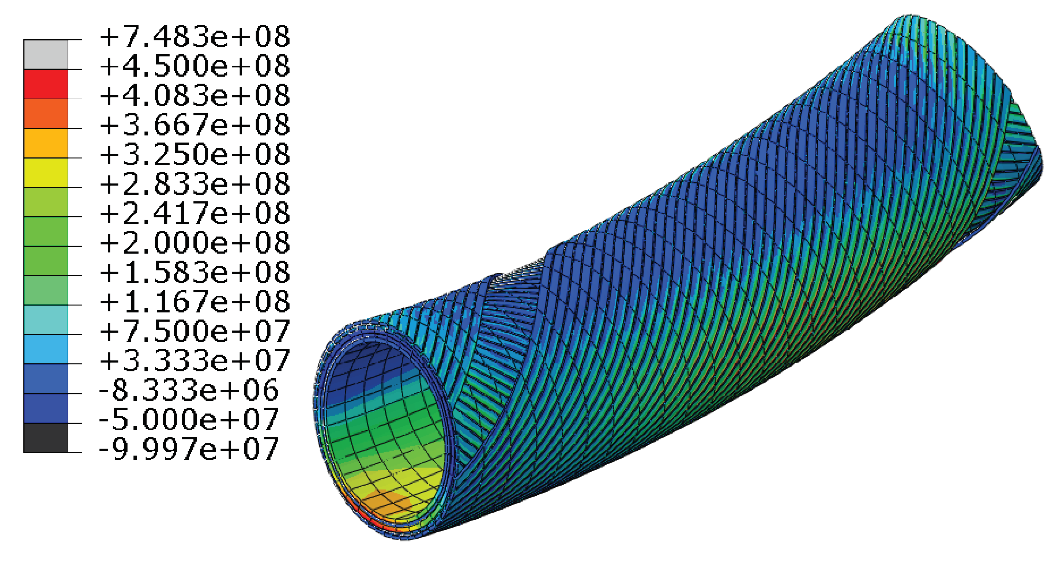
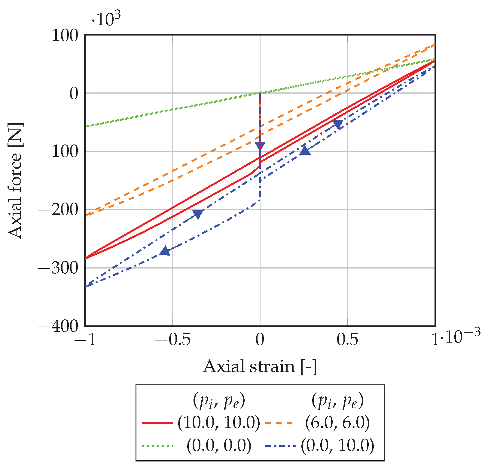
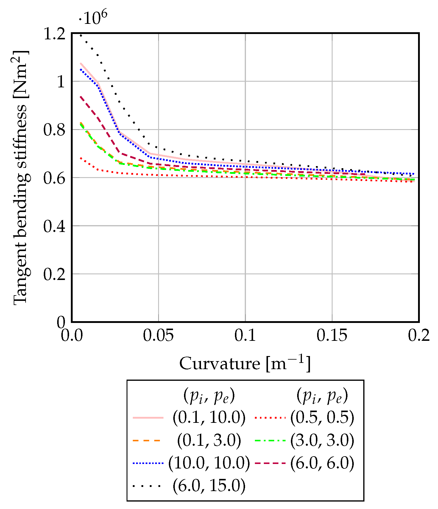
A set of axial, bending and torsional tests were carried out on the model to generate response data. Displacement control was used such that axial extension, torsion and net curvature in the pipe model were either constrained to be zero or prescribed to vary cyclically. Simulations were carried out on this model for a range of values of internal and external pressure. Selected axial, torsional and bending response data generated are shown in Figure 5, Figure 6 and Figure 7, respectively. (Refer to online version of this article for colored plots.) Typical stress results in the tensile wires are shown in Figure 4.

From the response plots, it is evident that pressure effects give rise to initial tension and torque, as well as increasing axial, torsional and bending stiffness. The increase in bending stiffness with pressure will lead to wider hysteresis loops under cyclic bending, which is consistent with results from cyclic bending tests reported by Skallerud [32] and Kebadze and Kraincanic [10] although Witz [11] shows results in which average bending stiffness is reduced at very high internal pressure. For local stress results, variation of stress across the width of tensile wires shows that local curvature effects are captured.

5. Multiscale Analysis Procedures

Due to the structural complexity of unbonded flexible risers, detailed FE modeling of full-length flexible pipes including individual riser layers is challenging and computationally expensive. A global-local modeling approach is therefore desirable. Multi-scale modeling of complex structures can follow a sequential local-global approach or a “nested approach”.

5.1. Sequential Multiscale Modeling

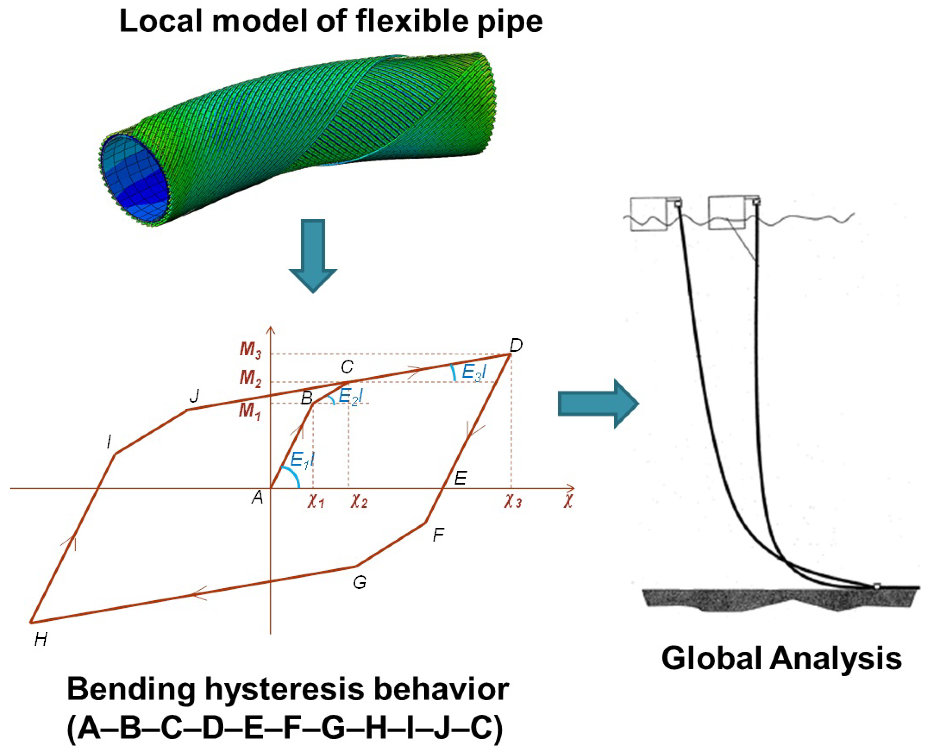
In a sequential multiscale approach, it is required that a suitable local time-invariant model is constructed and analysed to generate a set of responses under representative loading conditions. The responses obtained are then used to select and calibrate simpler representations for implementation in the global model, which can be modeled with homogenised representations, such as using idealized continuum models or structural elements, to estimate the global response. Subsequently, results obtained at selected points in the global analysis can be extracted and re-imposed on the local model as boundary conditions, enabling local stresses corresponding to the global motions to be determined. For a complex structure such as the multiple-layer flexible pipes considering layer interaction effects, a sequential approach is more practical for standard analyses. We demonstrate the sequential local-global approach for flexible pipes with local analyses of a length of flexible pipe using 3D FEA to determine the nonlinear responses under axial loading, torsion, bending moments and pressure (Figure 5, Figure 6 and Figure 7), followed by the global analyses of full-length flexible pipes with hybrid beam elements employing all constitutive behaviors obtained for each loading cases. The first part of this procedure is shown schematically in Figure 8: Simulations using the detailed finite element model are used to calibrate a constitutive model, which is then implemented in a large-scale simulation.

5.2. Nested Multiscale Modeling

For certain analyses in multiscale analysis, the sequential approach described above is inadequate, firstly because changes in the local state of the structure may affect the large-scale response and thus render the constitutive model calibration inaccurate, and secondly, because this influence on the large-scale response may in turn influence the state of the small-scale model. In flexible pipes, this includes the analysis of the consequences of wire breakage or loss of stability of the wires under pipe axial compression. These failure modes are discussed by Sousa et al. [14], de Sousa et al. [33] and Østergaard et al. [16], respectively. The development of a nested approach is considered valuable for studying such progressive damage modes and the effects of local damage and manufacturing errors on such instabilities. To analyse these situations, the following nested multi-scale framework is proposed.

In the nested approach, local detailed simulations of critical regions of the riser provide feedback to the global model in every load increment. The global model consists mostly of hybrid beam elements as used in the sequential global-local approach (described in Section 2), in which the axial, torsional and bending response is obtained from the constitutive model described in Section 3. At critical regions such as hang-off, touchdown point or areas where high curvature ranges are expected, “user multiscale elements” are employed instead of hybrid beam elements. These elements are associated with separate three-dimensional FEA representations of this pipe. Following the standard homogenisation terminology, these secondary models are referred to as Representative Volume Elements (RVE), as both their structure and response are representative of the local behavior of the structure at any point. If multiple multiscale elements are used, a separate set of local solution and state variables is stored for each so that local and global representations are updated consistently. The RVEs take displacements and rotations of the nodes of the multiscale elements as inputs for local simulations and return forces, moments and element tangent stiffness to the nodes of the multiscale element based on the results of the local simulations. Use of an incremental loading scheme in the global model and retention of RVE variables minimises the computational expense of such a scheme. Global load increment size influences the accuracy of the global response as it governs the update frequency of the multiscale elements. For models implemented in the Abaqus environment, execution control can be handled conveniently by a Python script while local variable storage can be achieved using analysis restarts.

5.3. RVE Analysis

An RVE model for flexible pipe was created taking into account interaction between pipe layers, as described in Section 4. For nested multiscale analysis, a truncated version of this model may be used, as suggested by Leroy and Estrier [13].

Traditionally, in computational homogenisation approaches for composite materials, either prescribed displacement boundary conditions, prescribed traction boundary conditions or periodic boundary conditions are applied when carrying out RVE analyses (see, for example, Geers et al. [25]). The most appropriate and convient choice for flexible pipes is periodic boundary conditions, due to the quasi-periodic nature of the structure. However, it is reconised that a primary determinant of flexible pipe global response and local stresses is the slip state of the helical armour wires, defined as the displacement of wire points relative to the deformation of the pipe structure (see, for example, Kebadze and Kraincanic [10]). Consequently, when initiating an RVE analysis, we are interested in imposing an overall deformation state (a combination of axial strain, bending and torsion), while implementing the assumption that the slip state of the helical wires varies periodically along the pipe as the circumferential coordinate of each point changes. This represents the conditions present in the pipe far from constrictions and terminations, and avoids over-constraining the model.

Conventional discrete periodic boundary conditions impose a set of constraints on a structure that can be written as

$$\begin{array}{c}\hfill u_i^L=u_i^R+u_i^{*}\end{array}$$

(26)

where $i=1,2,3$ denotes degrees of freedom, superscripts L and R indicate that the node belongs to the set of nodes on the left or right end of the structure, respectively, and $u^{*}$ represents the deformation state to be imposed on the model. Equation (26) must be enforced for every pair of discrete points in the model on the constrained surfaces.

We modify Equation (26) such that the imposed equality refers to displacements that are relative and expressed in a local basis:

$$\begin{array}{c}\hfill T_{ij}^L(u_j^1-u_j^2)=T_{ij}^R(u_j^3-u_j^4)+u_i^{*}\end{array}$$

(27)

In Equation (27), $T_{ij}$ is a basis transformation matrix $T_{ij}={\mathit{e}}_j·{\mathit{e}}_i$, superscripts 1 and 3 refer to constrained nodes as the left and right ends of the model, respectively, and superscripts 2 and 4 refer to displacements at the reference locations corresponding to the constrained nodes. This equation involves 4 points and must be repeated for every pair of discrete points in the model on the constrained surfaces. In finite element simulations, displacements $u_3$ and $u_4$ can be computed conviently by creating non-physical nodes that are forced by rigid body constraints to follow the pipe overall deformation,which is assumed to respond to the imposed axial strain, curvature and torsion as would an elastic cylinder. Imposition of pipe deformation and the periodic slip boundary conditions is achieved by chaining nodal degrees of freedom to a single control node. Following theoretical developments of computational homogenisation described by Edmans et al. [22], the work done at this node is equivalent to the work of the corresponding multiscale element.

5.4. Execution Control

Run-time linking between the RVE and global analyses is controlled by using Python scripting which automatically initializes the different global/local analyses and post-processes results. The RVE analysis is initialized by a Python sub-process command once each global load step is completed, which then provides the nodal displacements and rotations of the multiscale elements (special beam elements). A tracking method is used to indicate whether each global and local analysis are finished.

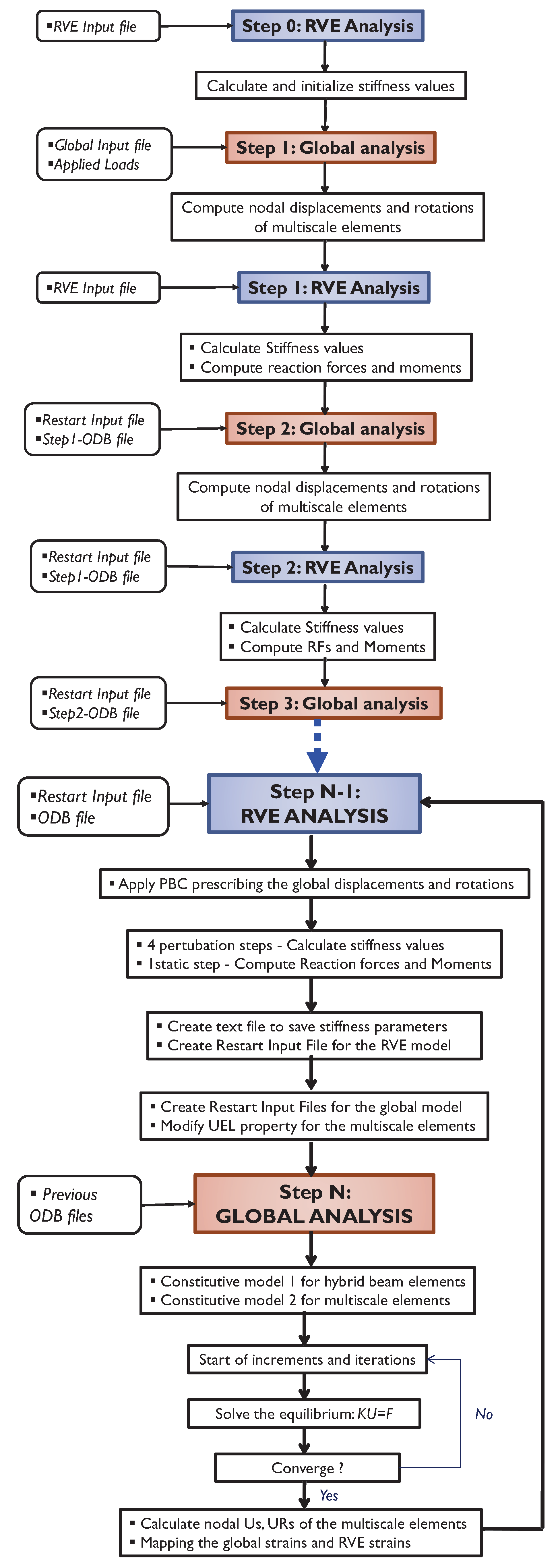
Each set of global displacements and rotations of the multiscale element’s nodes at every load increments is effectively transferred to the RVE model through Python scripting and application of periodic boundary conditions. On receiving the transferred deformation profiles, nonlinear analyses of the RVE are carried out to predict the 3D RVE deformation state corresponding to the current global step as well as to update the stiffness for the multiscale elements in the next load steps. Initial stiffnesses of the RVE are first calculated through a series of linear perturbation steps. The RVE perturbation analyses allow computation of the axial stiffness EA, bending stiffnesses EI1 and EI2, and torsional stiffness GJ at the current RVE deformed state without affecting the results of subsequent nonlinear analyses of the flexible pipe subject to the transferred global deformation. By this approach, we assume the stiffnesses of the RVE at the current state to be computed from the previous RVE deformation state. This is similar to the modified Newton iteration method whereby the stiffness matrices remains constant at the beginning the increment and only updated at the end of the increment. In addition, we develop a procedure to overwrite the stiffness of the global multiscale elements by those achieved from the RVE simulations. To handle various global and local analyses of the flexible pipe efficiently, we generate different restart analysis models for both the global and RVE models, storing all the previous deformed states and resume the analyses with new load information. Python scripting in association with shell batch scripts such as “Runjob.sh” and “Restart.sh” are implemented to run several simulation jobs at multiscale levels within a single execution command.

A flowchart for the complete nested multiscale framework is presented in Figure 9.

5.5. Verification of the Nested Multiscale Approach

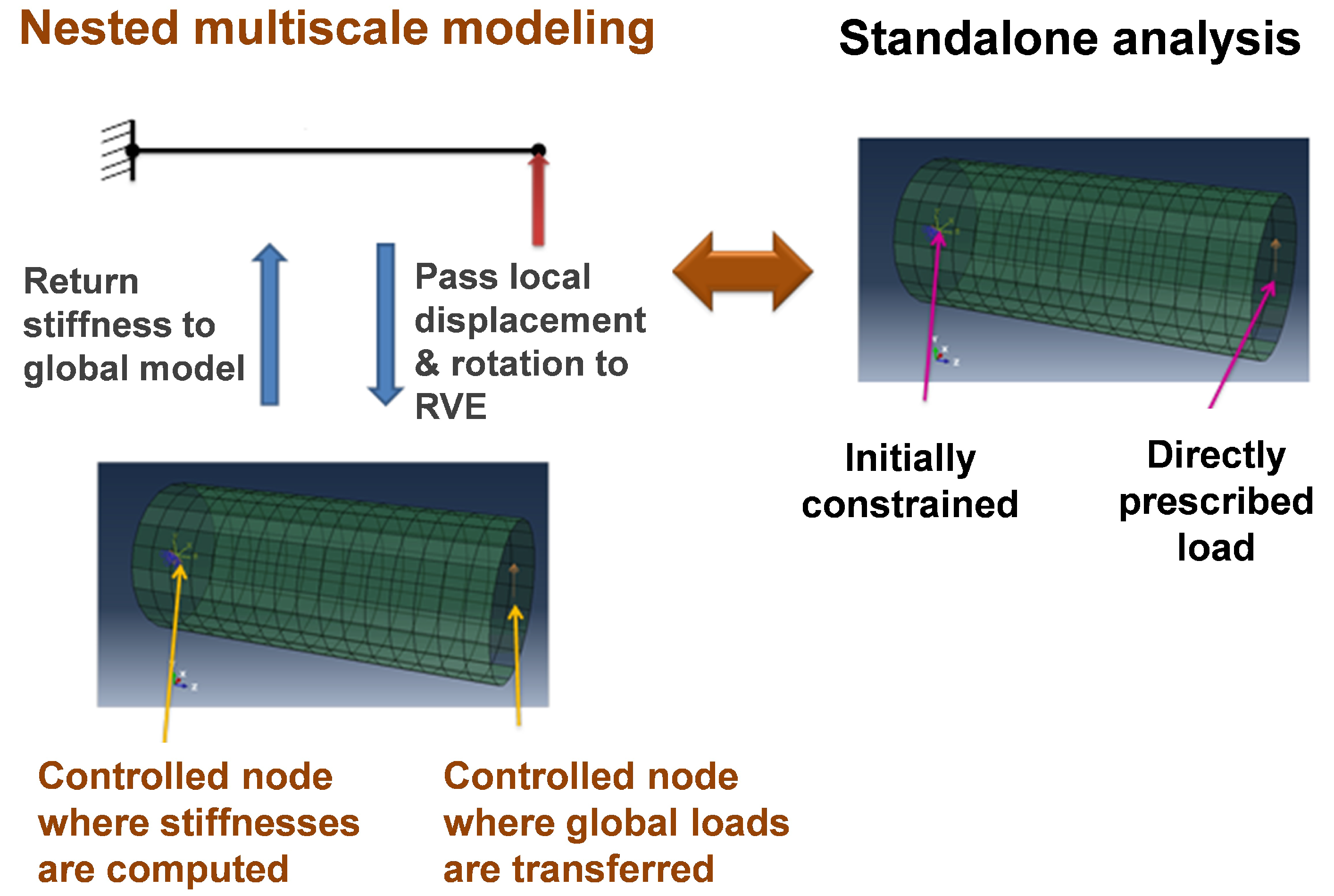
The application of the nested multiscale framework is demonstrated through simple examples of steel pipe models. The results of the integrated multiscale method are validated against the results of detailed and full-length analyses of pipes, referred to as “standalone analysis”, with identical material properties and loading conditions.

5.5.1. Example 1: Single Element

Using the nested multiscale approach, the global pipe model is defined with a single user-defined beam element (“multiscale element”) together with its associated RVE model. The pipe has an internal radius of 95.9 mm, an external radius of 116.2 mm and a length of 0.5 m. The RVE model associated with the multiscale element consists of 352 S4R shell elements. The internal and external radii and the pipe length of the RVE model are exactly the same as those of the single-beam global model. The validation is illustrated in Figure 10. This example is designed to validate the accuracy of the information passing framework and stiffness update procedure. Though this example is much simpler than an analysis of realistic flexible pipe, it provides a basis for validation efforts of the nested multiscale framework.

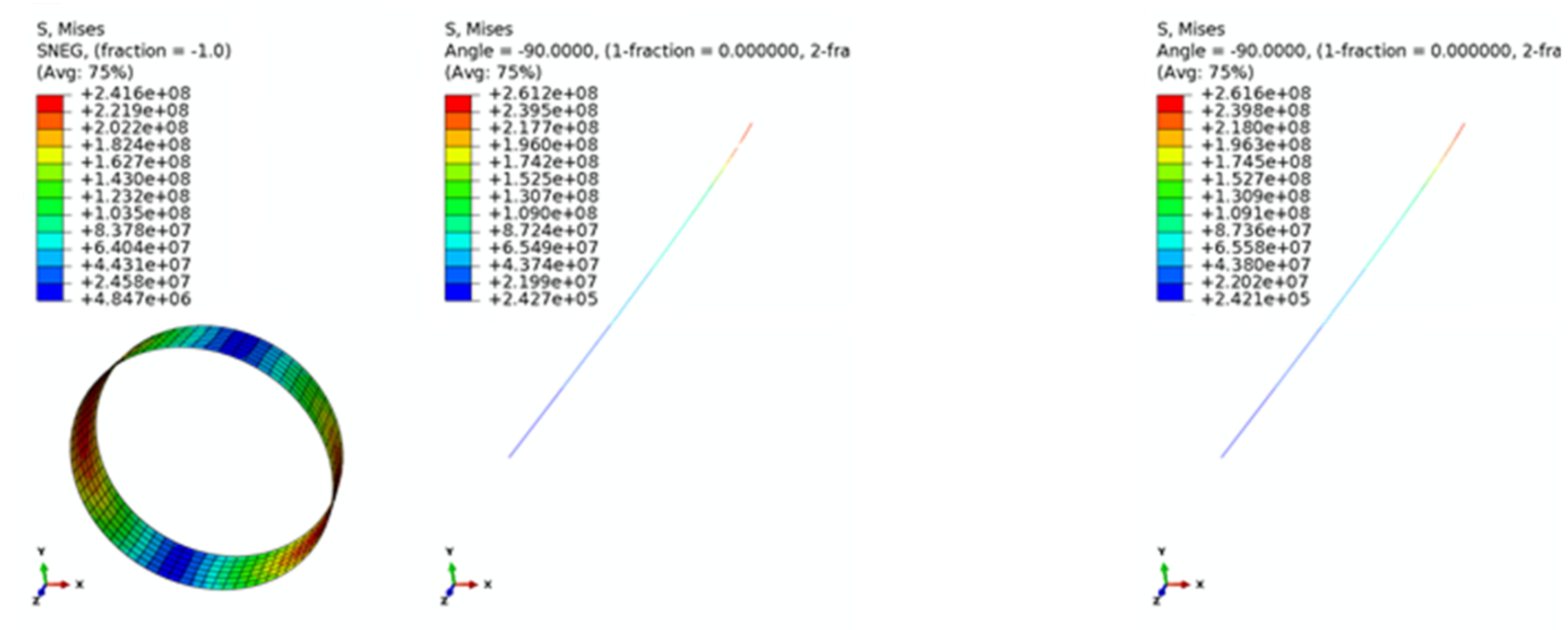
Comparison is made between the standalone analysis and the multiscale analysis. An elasto-plastic material model with elastic modulus of 200 GPa, yield stress of 250 MPa and an isotropic hardening of 2 GPa is used for both the standalone model and the RVE model. A vertical displacement is applied at one end of the global beam model while the rotations are fixed, and the response of the beam model and its associated RVE model are analysed. At every load increment, the global model transfers the displacements and rotations to the controlled nodes of the associated RVE of the multiscale element and obtains new stiffness values of RVE in return. The responses predicted for the pipe by the nested multiscale method is shown in Figure 11. It is seen that the results from the nested multiscale method are consistent with those predicted by the stand-alone analysis. The deformed shape of the pipe and the predicted Von Mises stress and plastic strains between the two models are identical.

5.5.2. Example 2: Multiple Elements

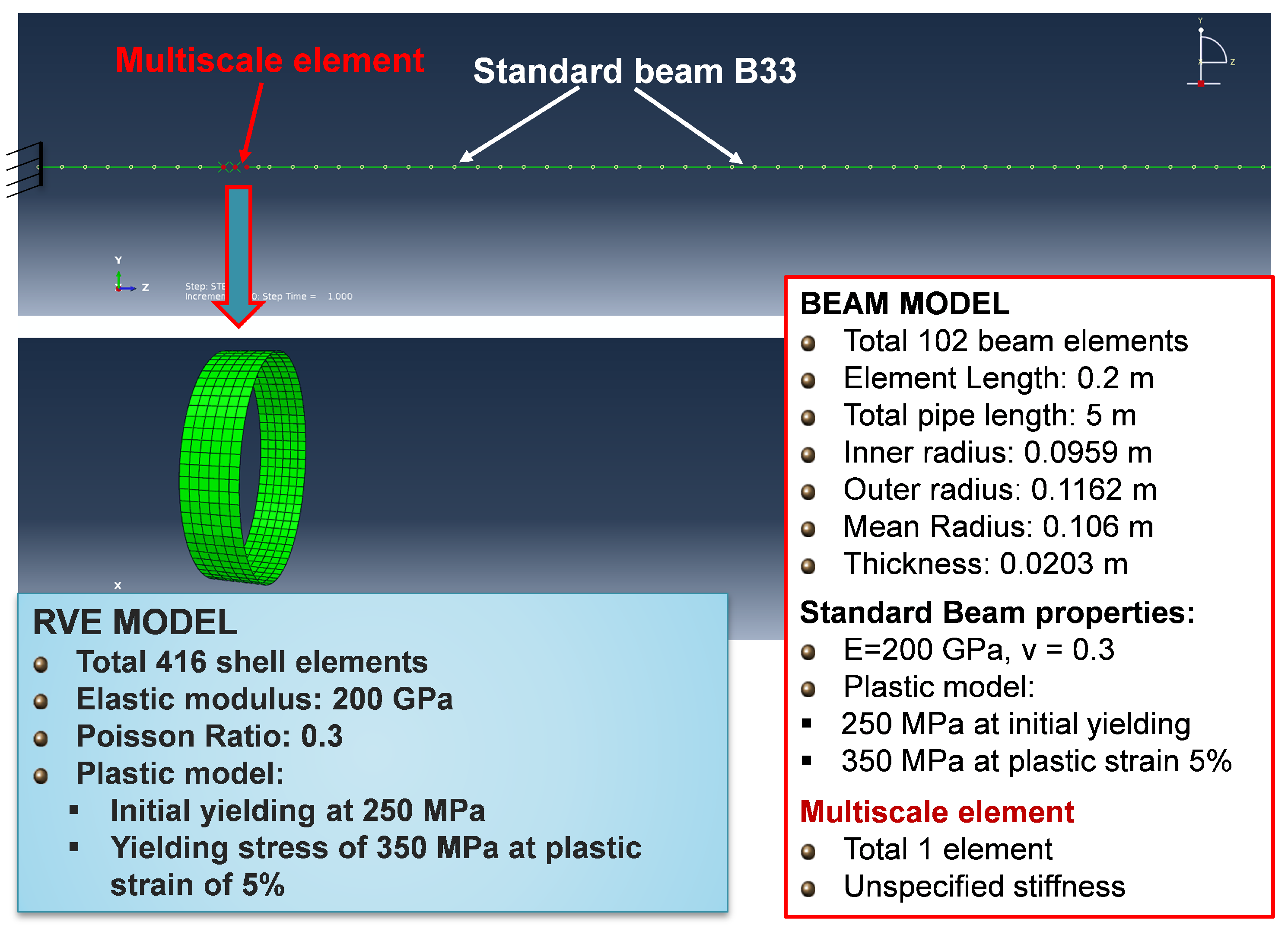
The multiscale model in this example consists of multiple standard beam elements (Abaqus B33 elements) and one multiscale element in the center. The standard beam B33 elements use the elastic-plastic material model as described in Example 1 while the constitutive model of the multiscale elements are obtained from its associated RVE model. A description of the global and RVE models for the nested multiscale method is shown in Figure 12. For comparison purposes, a standalone beam model, consisting solely of B33 elements is also analysed. The standalone model has the same pipe geometry and constitutive elastic-plastic behavior as the beam elements in the nested multiscale model. The left end of the beam is fixed while displacements in horizontal ($U_1$) and vertical ($U_2$) directions are applied to the right end of the beam

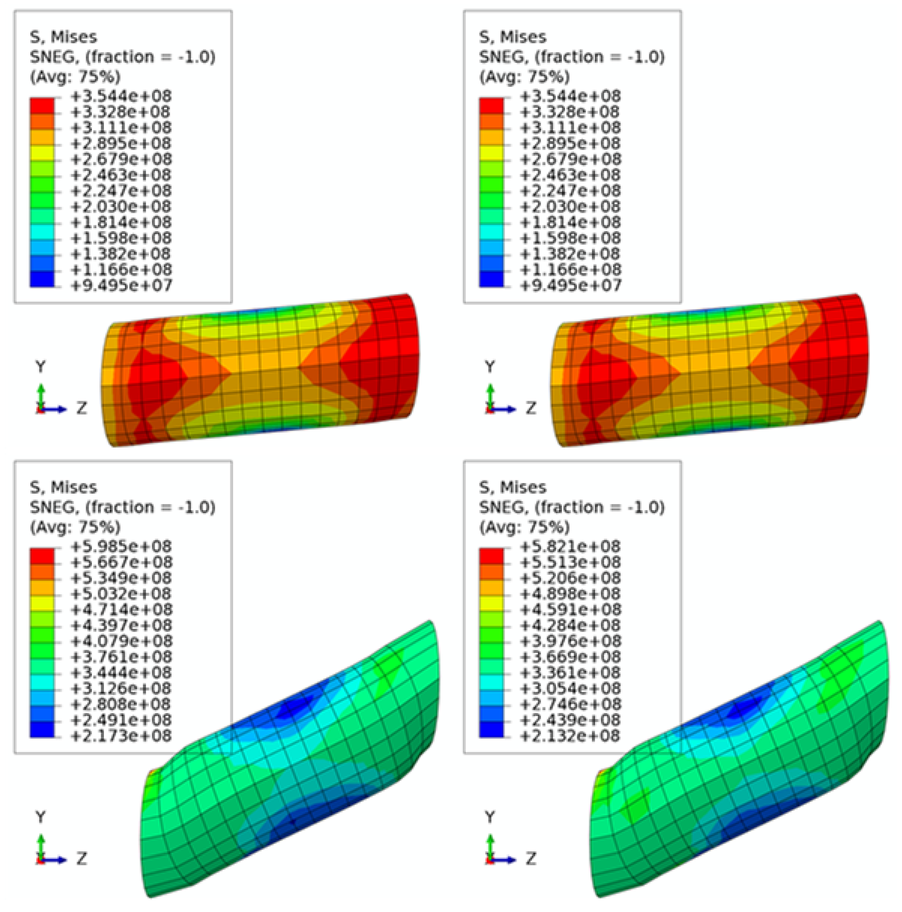
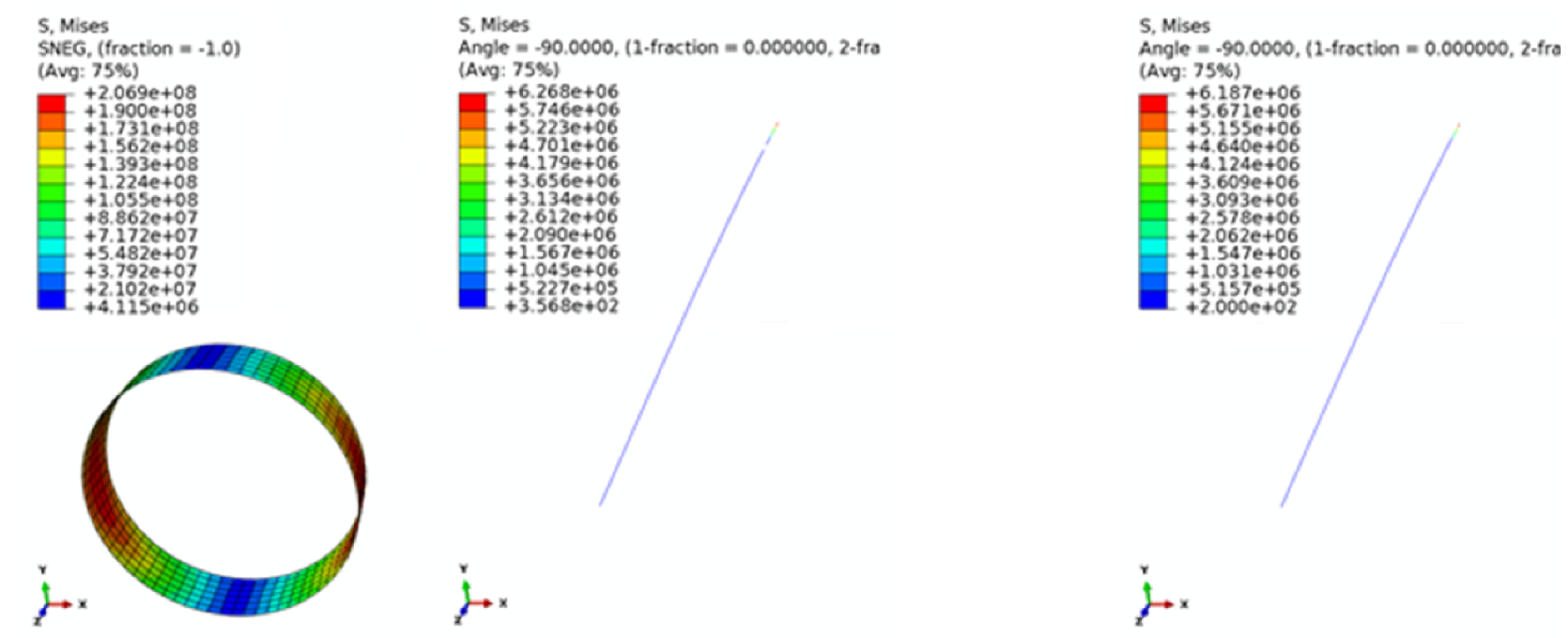
The results predicted by the standalone model and the integrated multiscale model are presented in Figure 13 and Figure 14. Comparison of plots in the center and right of each image shows good agreement between standalone and integrated approached. Similar values of maximum Von Mises stresses are obtained in the two models at different analysis steps, showing that the multiscale model is capable of providing consistent results with the standard beam model in Abaqus. It can also be observed that the nested multiscale method has an advantage over the standalone analysis in revealing more detailed stresses at the regions of interests through using multiscale elements, which becomes more relevant when increasingly complex structural models are investigated.

6. Verification of Dynamic Analysis Model

As part of efforts to demonstrate and validate these models, the dynamic analysis model was benchmarked against Orcaflex software. The scenario chosen for the comparison involved a tethered-wave configuration in shallow water attached to an FPSO subject to a regular Stokes 5th order wave. For comparison purposes, a linear elastic, decoupled section response model was employed in the beam element. The purpose of this verification is to demonstrate that the numerical formulation and treatment of hydrodynamic loads gives satisfactory results in a realistic dynamic analysis when compared to validated software using a different formulation (namely, a lumped-mass and -stiffness approach). Validation of the nonlinear section response model described in Section 3 is left for future work. A screenshot from the Orcaflex model showing the riser configuration shown in Figure 15.

Comparisons of effective tension range, static configuration and curvature range are shown in Figure 16, Figure 17 and Figure 18, respectively. For Figure 16 and Figure 18, curves represent maximum and minimum values obtained over the loading history (considering fully developed motion only) for each location along the riser arc length.

Based on the comparisons shown in Figure 16, Figure 17 and Figure 18, it can be concluded that the dynamic analysis implementation in Abaqus shows satisfactory agreement with Orcaflex.

7. Conclusions

In this article, procedures and methodologies for carrying out multiscale analysis of flexible risers have been presented. A detailed finite element model for local analysis, a beam element for global analysis and a nonlinear constitutive model have been introduced as component models. Procedures for carrying out sequential and integrated multiscale analyses have been described. The sequential procedure is distinguished from a standard global-local analysis by the inclusion of more realistic nonlinear behaviour in the global analysis that is tailored to the specific pipe design and operating conditions and the use of more accurate boundary conditions in the local analysis. The integrated procedure allows an evolving local configuration in selected elements to update the global analysis model in a staggered solution process. Applications of these multiscale procedures include fatigue assessment and, for the integrated model, investigation of progressive damage modes such as lateral buckling of tensile wires. Future validation work planned for this model include comparison of the global response obtained with the beam element/calibrated constitutive model against commercial dynamic analysis codes, as well as comparison of stresses obtained in the detailed FE model with other leading local analysis methods.

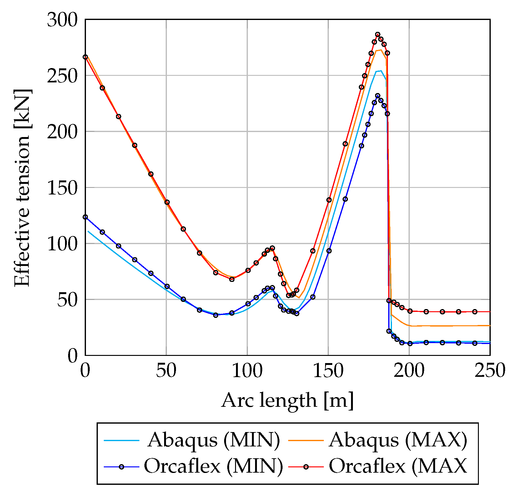
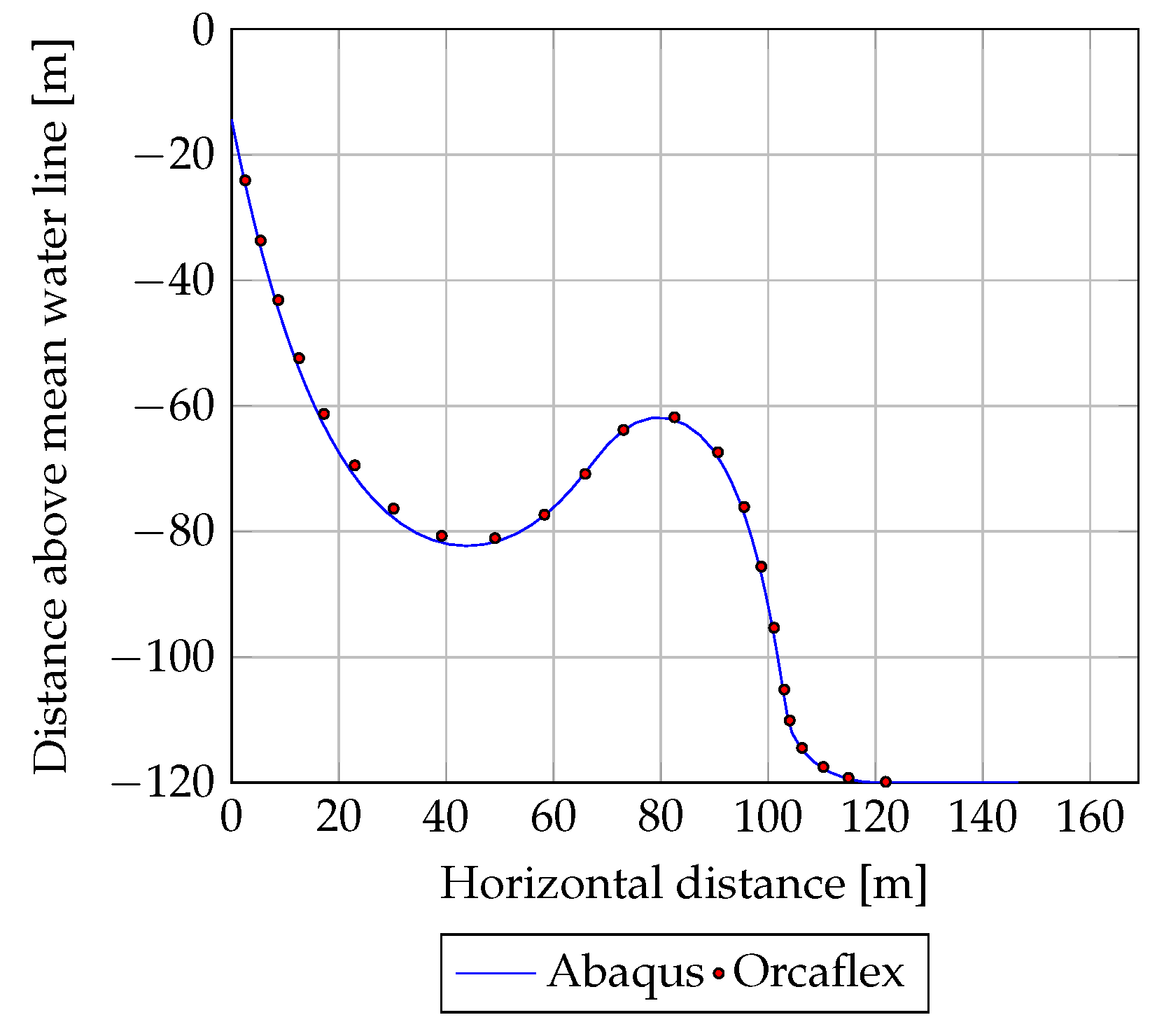
The adequacy of the lumped-mass and -stiffness approach used in Orcaflex for standalone dynamic analysis has been shown [35]. However, the authors contend that beam elements are more suitable for use in a multiscale framework. Beam elements allow the implementation of the wide variety of beam theories developed in structural mechanics and are formulated with reference to meaningful and measurable intermediate scale quantities (section force resultants and deformation measures). Consequently, we believe there is more scope for achieving a predictive and physically meaningful link between global dynamics and local stresses by using beam elements in global models. A survey of the performance of beam element formulations and/or beam theories for this application is outwith the scope of the current study. The current study demonstrated that a hybrid formulation with inextensibility constraint (Equation (11)) is an effective means of implementing beam theories in structures with high axial and low flexural stiffness. Further development of this approach could include implementation of more complex beam theories, in conjunction with determination of other section deformation measures (such as section rotation and warping).

References

1. Edmans, B.; Alfano, G.; Bahai, H. Large-scale analysis and local stress assessment of flexible unbonded pipes using FEA. In Proceedings of the ASME 2012 31st International Conference on Ocean, Offshore and Arctic Engineering, Rio de Janeiro, Brazil, 1–6 July 2012; The American Society of Mechanical Engineers (ASME): New York, NY, USA, 2012; Volume 3, pp. 947–953. [Google Scholar] [CrossRef]
2. Pham, D.C.; Sridhar, N.; Qian, X.; Sobey, A.; Achintha, M.; Shenoi, A. A review on design, manufacture and mechanics of composite risers. Ocean Eng. 2016, 112, 82–96. [Google Scholar] [CrossRef] [Green Version]
3. Sun, X.; Chen, Y.; Tan, V.; Jaiman, R.; Tay, T. Homogenization and stress analysis of multilayered composite offshore production risers. J. Appl. Mech. Trans. ASME 2014, 81. [Google Scholar] [CrossRef]
4. Amaechi, C.V.; Gillett, N.; Odijie, A.C.; Hou, X.; Ye, J. Composite risers for deep waters using a numerical modelling approach. Compos. Struct. 2019, 210, 486–499. [Google Scholar] [CrossRef]
5. McNamara, J.F.; O’Brien, P.; Gilroy, S. Nonlinear analysis of flexible risers using hybrid finite elements. J. Offshore Mech. Arct. Eng. 1988, 110, 197–204. [Google Scholar] [CrossRef]
6. Yazdchi, M.; Crisfield, M. Buoyancy forces and the 2D finite element analysis of flexible offshore pipes and risers. Int. J. Numer. Methods Eng. 2002, 54, 66–81. [Google Scholar] [CrossRef]
7. Yazdchi, M.; Crisfield, M. Non-linear dynamic behaviour of flexible marine pipes and risers. Int. J. Numer. Methods Eng. 2002, 54, 1265–1308. [Google Scholar] [CrossRef]
8. Monprapussorn, T.; Chucheepsakul, S.; Huang, T. The coupled radial-axial deformations analysis of flexible pipes conveying fluid. Int. J. Numer. Methods Eng. 2004, 59, 1399–1452. [Google Scholar] [CrossRef]
9. McNamara, J.; Harte, A. Three dimensional analytical simulation of flexible pipe wall structure. Proc. Int. Offshore Mech. Arct. Eng. Symp. 1989, 1, 477–482. [Google Scholar] [CrossRef]
10. Kebadze, E.; Kraincanic, I. Nonlinear Bending Behavior of Offshore Flexible Pipe. In Proceedings of the International Offshore and Polar Engineering Conference, Brest, France, 30 May–4 June 1999; International Society of Offshore and Polar Engineers (ISOPE): Mountain View, CA, USA, 1999; Volume 2. [Google Scholar]
11. Witz, J.A. A case study in the cross-section analysis of flexible risers. Mar. Struct. 1996, 9, 885–904. [Google Scholar] [CrossRef]
12. Tan, Z.; Case, M.; Sheldrake, T. Higher Order Effects on Bending of Helical Armour Wire Inside an Unbonded Flexible Pipe. In Proceedings of the ASME 2005 24th International Conference on Ocean, Offshore and Arctic Engineering, Halkidiki, Greece, 12–17 June 2015; The American Society of Mechanical Engineers (ASME): New York, NY, USA, 2005. [Google Scholar]
13. Leroy, J.; Estrier, P. Stress Assessment in Armour Wires of Flexible Risers. In Proceedings of the ASME 2010 29th International Conference on Ocean, Offshore and Arctic Engineering, Shanghai, China, 6–11 June 2010; The American Society of Mechanical Engineers (ASME): New York, NY, USA, 2010. [Google Scholar]
14. Sousa, J.; de Sousa, F.J.M.; Siqueira, M.Q. Fatigue Analysis of a 6″Flexible Pipe with Broken Tensile Armour Wires. In Proceedings of the ASME 2012 31st International Conference on Ocean, Offshore and Arctic Engineering, Rio de Janeiro, Brazil, 1–6 July 2012; The American Society of Mechanical Engineers (ASME): New York, NY, USA, 2012. [Google Scholar]
15. Sævik, S. Theoretical and experimental studies of stresses in flexible pipes. Comput. Struct. 2011, 89, 2271–2291. [Google Scholar] [CrossRef]
16. Østergaard, N.H.; Lyckegaard, A.; Andreasen, J.H. A method for prediction of the equilibrium state of a long and slender wire on a frictionless toroid applied for the analysis of flexible pipe structures. Eng. Struct. 2012, 34, 391–399. [Google Scholar] [CrossRef]
17. Caleyron, F.; Guiton, M.; Leroy, J.M.; Perdizet, T.; Charliac, D.; Estrier, P.; Paumier, L. A Multi-Purpose Finite Element Model for Flexible Risers Studies. In Proceedings of the ASME 2014 33rd International Conference on Ocean, Offshore and Arctic Engineering, San Francisco, CA, USA, 8–13 June 2014; The American Society of Mechanical Engineers (ASME): New York, NY, USA, 2014. [Google Scholar]
18. Majed, A.; Bhat, S.; Dib, M.; Cooper, P. A nonlinear dynamic substructuring approach for efficient detailed global analysis of flexible risers. In Proceedings of the Offshore Technology Conference, Houston, TX, USA, 6–9 May 2013. [Google Scholar]
19. Edmans, B.; Pham, D.C.; Zhang, Z.Q.; Guo, T.F.; Sridhar, N.; Stewart, G. Multiscale Finite Element Analysis of Unbonded Flexible Risers. In Proceedings of the ASME 2014 33rd International Conference on Ocean, Offshore and Arctic Engineering, San Francisco, CA, USA, 8–13 June 2014; The American Society of Mechanical Engineers (ASME): New York, NY, USA, 2014. [Google Scholar] [Green Version]
20. Pham, D.C.; Guo, T.F.; Zhang, Z.Q.; Narayanaswamy, S.; Edmans, B. An Effective Constitutive Model for Unbonded Flexible Risers. In Proceedings of the Annual Offshore Technology Conference, Kuala Lumpur, Malaysia, 25–28 March 2014; Society of Petroleum Engineers: London, UK, 2014; Volume 3, pp. 2456–2465. [Google Scholar]
21. Pham, D.C.; Guo, T.F.; Zhang, Z.Q.; Narayanaswamy, S.; Edmans, B. Multiscale Modelling Approaches for Flexible Risers: Procedures, Capabilities and Demonstrations. In Proceedings of the Annual Offshore Technology Conference, Kuala Lumpur, Malaysia, 22–25 March 2016; Society of Petroleum Engineers: London, UK, 2016. [Google Scholar]
22. Edmans, B.; Alfano, G.; Bahai, H. Nonlinear multi-scale homogenization with different structural models at different scales. Int. J. Numer. Methods Eng. 2013, 94, 355–373. [Google Scholar] [CrossRef] [Green Version]
23. Tay, T.E.; Liu, G.; Tan, V.; Sun, X.; Pham, D.C. Progressive failure analysis of composites. J. Compos. Mater. 2008, 42, 1921–1966. [Google Scholar] [CrossRef]
24. Pham, D.C.; Sun, X.; Tan, V.; Chen, B.; Tay, T.E. Progressive failure analysis of scaled double-notched carbon/epoxy composite laminates. Int. J. Damage Mech. 2012, 21, 1154–1185. [Google Scholar] [CrossRef]
25. Geers, M.; Kouznetsova, V.; Brekelmans, W. Multi-scale computational homogenisation: Trends and challenges. J. Comput. Appl. Math. 2010, 234, 2175–2182. [Google Scholar] [CrossRef]
26. Sacco, E. A nonlinear homogenisation procedure for periodic masonry. Eur. J. Mech. A Solids 2009, 28, 209–222. [Google Scholar] [CrossRef]
27. Battini, J. Corotational Beam Elements in Instability Problems. Ph.D. Thesis, Department of Civil and Architectural Engineering, KTH Royal Institute of Technology, Stockholm, Sweden, 2002. [Google Scholar]
28. Crisfield, M. Non-Linear Finite Element Analysis of Solids and Structures; John Wiley & Sons Ltd: Hoboken, NJ, USA, 2000. [Google Scholar]
29. Le, T. Corotational Formulation for Nonlinear Dynamic Analysis of Flexible Beam Structures. Ph.D. Thesis, KTH Royal Institute of Technology, Stockholm, Sweden, 2012. [Google Scholar]
30. Dassault Systèmes, A. Abaqus Theory Guide; Dassault Systemes Simulia Corp.: Providence, RI, USA, 2011. [Google Scholar]
31. Puzrin, A.M.; Houlsby, G.T. Fundamentals of kinematic hardening hyperplasticity. Int. J. Soilds Struct. 2001, 38, 3771–3794. [Google Scholar] [CrossRef]
32. Skallerud, B. Structural Damping in a Wellstream Pipe; Technical Report; Report STF71 F91059; SINTEF: Trondheim, Norway, 1991. [Google Scholar]
33. de Sousa, J.R.M.; Campello, G.C.; Bueno, A.F.B.; Vardaro, E.; Ellwanger, G.B.; Strohaecker, T.R. On the Structural Response of a Flexible Pipe With Damaged Tensile Armour Wires. In Proceedings of the ASME 2011 30th International Conference on Ocean, Offshore and Arctic Engineering, Rotterdam, The Netherlands, 19–24 June 2011; The American Society of Mechanical Engineers (ASME): New York, NY, USA, 2011; pp. 847–858. [Google Scholar]
34. Pham, D.C.; Zhang, Z.Q.; Guo, T.F.; Sridhar, N.; Edmans, B.; Stewart, G. Multiscale Modeling Approach for Flexible Riser. In Proceedings of the 20th International Conferences on Composite Material (ICCM20), Copenhagen, Denmark, 19–24 July 2015; ICCM: London, UK, 2015. [Google Scholar]
35. Orcina, L. Deepwater SCR Comparison with Flexcom; Technical Report 99/101; Orcina, Ltd.: Ulverston, UK, 2018. [Google Scholar]
Figure 1. Typical flexible pipe internal structure (Source: GE Oil and Gas).
Jmse 07 00340 g001
Figure 2. Beam kinematics and co-rotational coordinate systems.
Jmse 07 00340 g002
Figure 3. Euler-Bernoulli beam with center-line resultants.
Jmse 07 00340 g003
Figure 4. Maximum principal stress (radius of curvature = 5m, p i = 6 MPa, p e = 15 MPa, displacement exaggerated by factor of 3.0. Outer sheath, anti-wear layer and some outer tensile wires removed.).
Jmse 07 00340 g004
Figure 5. Axial results. Pressures in MPa.
Jmse 07 00340 g005
Figure 6. Torsional results. Pressures in MPa.
Jmse 07 00340 g006
Figure 7. Bending results.
Jmse 07 00340 g007
Figure 8. Sequential analysis of flexible pipe.
Jmse 07 00340 g008
Figure 9. Flowchart for nested multiscale procedure.
Jmse 07 00340 g009
Figure 10. Multiscale validation: Example 1.
Jmse 07 00340 g010
Figure 11. Von Mises Stress prediction by the nested multiscale method (on the left) and stand-alone RVE analysis (on the right) at different global steps. (a) (above) with applied vertical load U 2 = 0.05 m ; (b) (below) with applied vertical load U 2 = 0.25 m.
Jmse 07 00340 g011
Figure 12. Description of the nested multiscale model with standard beam elements B33 and one multiscale element with its associated RVE (reproduced from Pham et al. [34], with permission).
Jmse 07 00340 g012
Figure 13. Comparison on Von Mises Stress between the nested multiscale method (left and center) and stand-alone beam B33 analysis (right) at U 1 = 0.2 m, U 2 = 0.0 m.
Jmse 07 00340 g013
Figure 14. Comparison on Von Mises Stress between the nested multiscale method (left and center) and stand-alone beam B33 analysis (right) at U 1 = −0.2 m, U 2 = 0.2 m.
Jmse 07 00340 g014
Figure 15. Orcaflex model configuration used for validation of dynamic analysis, showing FPSO, buoyancy modules and hold-down tether.
Jmse 07 00340 g015
Figure 16. Abaqus-Orcaflex comparison: Riser effective tension range. Z-direction is vertical in global system.
Jmse 07 00340 g016
Figure 17. Abaqus-Orcaflex comparison: Riser static configuration.
Jmse 07 00340 g017
Figure 18. Abaqus-Orcaflex comparison: Riser curvature range.
Jmse 07 00340 g018