Modeling Analysis and Simulation of Viscous Hydrodynamic Model of Single-DOF Manipulator

Abstract

Hydrodynamic modeling is the basis of the precise control research of underwater manipulators. Viscous hydrodynamics, an important part of the hydrodynamic model, directly affects the accuracy of the dynamic model and the control model of the manipulator. Considering the limited research on viscous hydrodynamics of underwater manipulators and the difficulty in measuring viscous hydrodynamic coefficients, the viscous hydrodynamic model in the form of Taylor expansion is analyzed and established. Through carrying out simulation calculations, curve fitting and regression analysis, positional derivatives, rotational derivatives, and coupling derivatives in the viscous hydrodynamic model, are determined. This model provides a crucial theoretical foundation and reference data for subsequent related research.

1. Introduction

With the rapid development of the marine industry, the application of robots mounted on underwater vehicles has become increasingly widespread. Underwater manipulators are mainly employed in the acquisition and exploration, etc. Their underwater performance can be determined by their speed and accuracy. Underwater manipulators are usually subjected to large forces and moments during their operation. These forces and moments mainly include gravity, inertial hydrodynamics, and viscous hydrodynamics. There are more solutions to the determination of gravity and inertial hydrodynamics. Therefore, the viscous hydrodynamic model has become a research focus that needs to be broken through because of its large number of coefficients and the difficulty of measurement.

References [1,2,3] verified the accuracy of fluid simulation calculations using software, such as FLUENT, by comparing the simulated calculation values of hydrodynamics with the measured values of engineering methods. References [4,5,6] studied the drag and additional mass force of the manipulator underwater and obtained the inertial hydrodynamic model by the CFD (Computational Fluid Dynamics) simulation, but the viscous hydrodynamics were not considered as key targets in the study. References [7,8,9,10] numerically calculated the viscous hydrodynamic coefficients of submarine and ship models with complex shapes under the specified navigation conditions and further improved the handling performance during navigation. Reference [11] determined the viscous kinetic coefficients of the manipulator through aerodynamic experiments and carried out a sea trial.

At present, research on viscous hydrodynamics mostly focus on specific ship models and underwater vehicles, and less on manipulators loaded on them. Therefore, a numerical calculation method of the viscous hydrodynamic coefficient based on single-DOF (Degree of Freedom) manipulators is put forward. The method is based on ANSYS Fluent. UDF (user-defined function) and dynamic mesh which are used to simulate the rotational motion of the manipulator. The inlet and outlet conditions, as well as boundary conditions of the fluid domain, are changed. Also, the viscous hydrodynamic model could be obtained by curve fitting and regression analysis.

2. Mathematical Model and Theoretical Analysis

2.1. Mathematical Modeling of Viscous Hydrodynamics

Since its surrounding flow field is changed during the operation of the underwater manipulator; the arm is subjected to the reaction of the water body caused by force generated by the water body. The hydrodynamics of the moving manipulator in water include two parts: Inertial hydrodynamics caused by acceleration and viscous hydrodynamics caused by friction. Inertial hydrodynamics is generally determined by empirical formulas, while coefficients of viscous hydrodynamics are complex and difficult to measure.

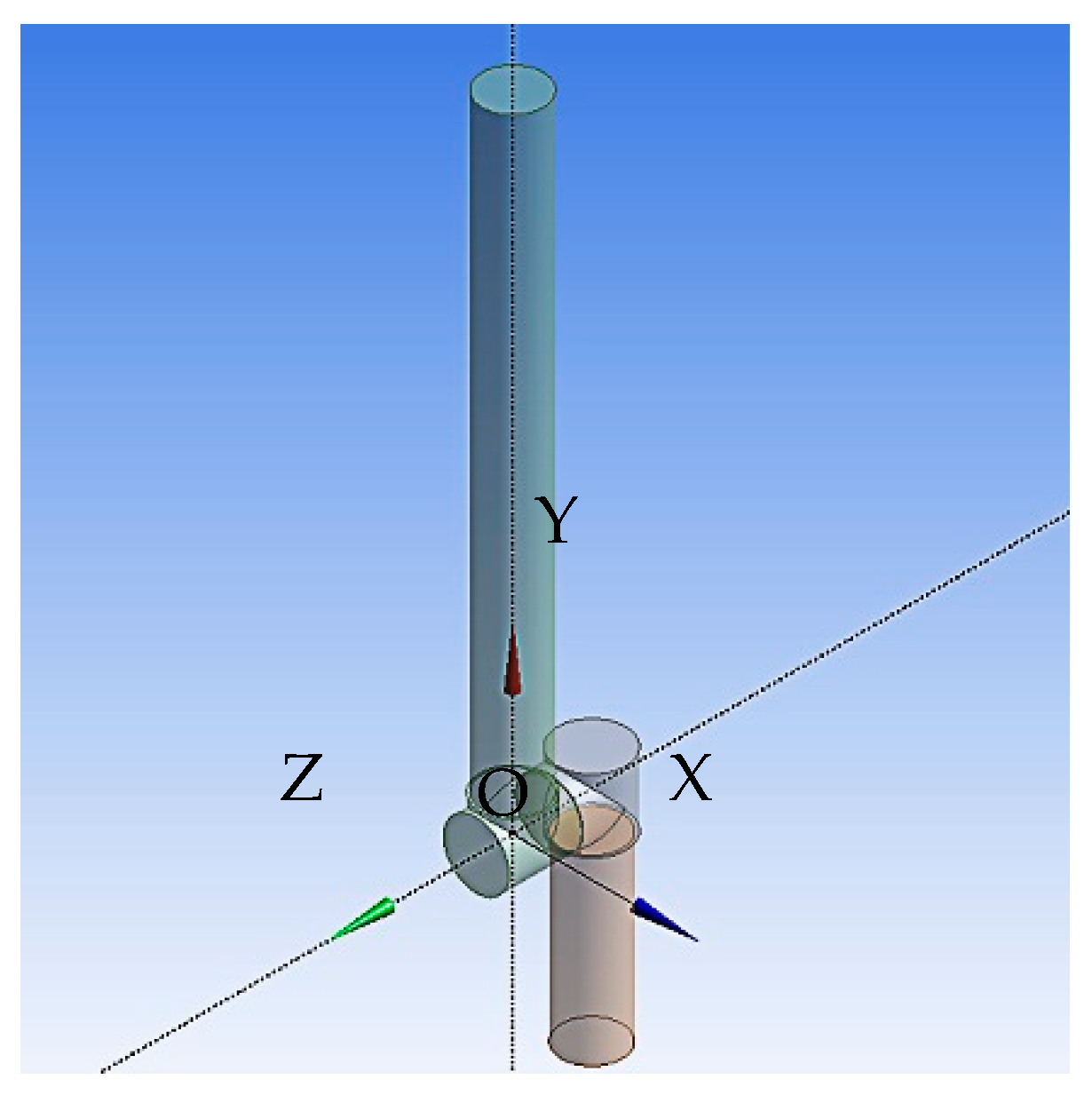
This paper is intended to use a single-DOF manipulator model mounted on a fixed base. The arm is a homogeneous lightweight rod with a circular cross-section, 50 mm in diameter (d), 500 mm in arm length (l), at length to diameter ratio of 10, belonging to the slender pole. The establishment of its coordinate system is shown in Figure 1.

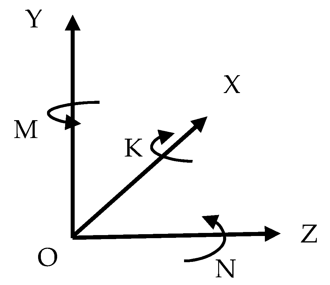
When the manipulator performs the constant motion, the influence of acceleration and angular acceleration on the motion variable could be ignored based on the “slow-motion” assumption. So the mere considerations for viscous hydrodynamics are the effects of the velocity and angular velocity in the motion variable. It can be represented as: $\mathrm{U}={\left[\mathrm{u}\mathrm{v}\mathrm{w}\mathrm{p}\mathrm{q}\mathrm{r}\right]}^{\mathrm{T}}$, where u stands for the velocity in the OX direction, v for the velocity in the OY direction, w for the velocity in the OZ direction, p for the angular velocity of the rotation around the OX axis, q for the angular velocity of the rotation around the OY axis, and r for the angular velocity of the rotation around the OZ axis.

The viscous hydrodynamics can be expressed as a multivariate function $\mathrm{F}=\mathrm{f}\left(\mathrm{u},\mathrm{v},\mathrm{w},\mathrm{p},\mathrm{q},\mathrm{r}\right)$, and the six-dimensional component of viscous hydrodynamics $\mathrm{F}={\left[\mathrm{X}\mathrm{Y}\mathrm{Z}\mathrm{K}\mathrm{M}\mathrm{N}\right]}^{\mathrm{T}}$ could also be displayed in the above functional form, the direction of which is shown in Figure 2.

The viscous hydrodynamic F performs Taylor expansion in the form of Equation (1):

$$\begin{array}{ll}\mathrm{f}\left(\mathrm{U}\right)=& \mathrm{f}\left({\mathrm{U}}_{\mathrm{k}}\right)+{\left(\mathrm{U}-{\mathrm{U}}_{\mathrm{k}}\right)}^{\mathrm{T}}\nabla \mathrm{f}\left({\mathrm{U}}_{\mathrm{k}}\right)\\ & +\frac{1}{2!}{\left(\mathrm{U}-{\mathrm{U}}_{\mathrm{k}}\right)}^{\mathrm{T}}\mathrm{H}\left({\mathrm{U}}_{\mathrm{k}}\right)\left(\mathrm{U}-{\mathrm{U}}_{\mathrm{k}}\right)+o^{\mathrm{n}}\end{array}$$

(1)

where ${\mathrm{U}}_{\mathrm{k}}={\left[{\mathrm{u}}_0{\mathrm{v}}_0{\mathrm{w}}_0{\mathrm{p}}_0{\mathrm{q}}_0{\mathrm{r}}_0\right]}^{\mathrm{T}}$, ${\mathrm{U}}_{\mathrm{k}}$ is the initial constant.

$$\mathrm{H}\left({\mathrm{U}}_{\mathrm{k}}\right)=\left[\begin{array}{cccc}\frac{{\partial }^2\mathrm{f}\left({\mathrm{U}}_{\mathrm{k}}\right)}{\partial {\mathrm{u}}^2}& \frac{{\partial }^2\mathrm{f}\left({\mathrm{U}}_{\mathrm{k}}\right)}{\partial \mathrm{u}\partial \mathrm{v}}& \cdots & \frac{{\partial }^2\mathrm{f}\left({\mathrm{U}}_{\mathrm{k}}\right)}{\partial \mathrm{u}\partial \mathrm{r}}\\ \frac{{\partial }^2\mathrm{f}\left({\mathrm{U}}_{\mathrm{k}}\right)}{\partial \mathrm{u}\partial \mathrm{v}}& \frac{{\partial }^2\mathrm{f}\left({\mathrm{U}}_{\mathrm{k}}\right)}{\partial {\mathrm{v}}^2}& \cdots & \frac{{\partial }^2\mathrm{f}\left({\mathrm{U}}_{\mathrm{k}}\right)}{\partial \mathrm{v}\partial \mathrm{r}}\\ ⋮& ⋮& \ddots & ⋮\\ \frac{{\partial }^2\mathrm{f}\left({\mathrm{U}}_{\mathrm{k}}\right)}{\partial \mathrm{u}\partial \mathrm{r}}& \frac{{\partial }^2\mathrm{f}\left({\mathrm{U}}_{\mathrm{k}}\right)}{\partial \mathrm{v}\partial \mathrm{r}}& \cdots & \frac{{\partial }^2\mathrm{f}\left({\mathrm{U}}_{\mathrm{k}}\right)}{\partial {\mathrm{r}}^2}\end{array}\right]$$

Considering the left-right and front-back symmetry and the motion limit of the manipulator, several coefficients in the second-order expansions are zero, and the remaining others are non-negligible hydrodynamic coefficients, as in Equation (2):

$$\{\begin{array}{l}{\mathrm{X}=\mathrm{X}}_{\mathrm{uu}}{\mathrm{u}}^2+{\mathrm{X}}_{\mathrm{vv}}{\mathrm{v}}^2+{\mathrm{X}}_{\mathrm{ww}}{\mathrm{w}}^2+{\mathrm{X}}_{\mathrm{rr}}{\mathrm{r}}^2+{\mathrm{X}}_{\mathrm{vr}}\mathrm{vr}\\ {\mathrm{Y}=\mathrm{Y}}_{\mathrm{v}}\mathrm{v}+{\mathrm{Y}}_{\mathrm{r}}\mathrm{r}+{\mathrm{Y}}_{\mathrm{v}\left|\mathrm{v}\right|}\mathrm{v}\left|\mathrm{v}\right|{+\mathrm{Y}}_{\mathrm{r}\left|\mathrm{r}\right|}\mathrm{r}\left|\mathrm{r}\right|{+\mathrm{Y}}_{\mathrm{v}\left|\mathrm{r}\right|}\mathrm{v}\left|\mathrm{r}\right|\\ {\mathrm{Z}=\mathrm{Z}}_{\mathrm{w}}\mathrm{w}+{\mathrm{Z}}_{\mathrm{w}\left|\mathrm{w}\right|}\mathrm{w}\left|\mathrm{w}\right|+{\mathrm{Z}}_{\mathrm{vv}}{\mathrm{v}}^2+{\mathrm{Z}}_{\mathrm{rr}}{\mathrm{r}}^2+{\mathrm{Z}}_{\mathrm{vr}}\mathrm{vr}\\ {\mathrm{K}=\mathrm{K}}_{\mathrm{v}}\mathrm{v}+{\mathrm{K}}_{\mathrm{v}\left|\mathrm{v}\right|}{\mathrm{v}+\mathrm{K}}_{\mathrm{r}}{\mathrm{r}+\mathrm{K}}_{\mathrm{r}\left|\mathrm{r}\right|}\mathrm{r}\left|\mathrm{r}\right|\\ {\mathrm{M}=\mathrm{M}}_{\mathrm{w}}\mathrm{w}+{\mathrm{M}}_{\mathrm{w}\left|\mathrm{w}\right|}\mathrm{w}\left|\mathrm{w}\right|+{\mathrm{M}}_{\mathrm{vv}}{\mathrm{v}}^2+{\mathrm{M}}_{\mathrm{rr}}{\mathrm{r}}^2+{\mathrm{M}}_{\mathrm{vr}}\mathrm{vr}\\ {\mathrm{N}=\mathrm{N}}_{\mathrm{v}}\mathrm{v}+{\mathrm{N}}_{\mathrm{r}}\mathrm{r}+{\mathrm{N}}_{\mathrm{v}\left|\mathrm{v}\right|}\mathrm{v}\left|\mathrm{v}\right|+{\mathrm{N}}_{\mathrm{r}\left|\mathrm{r}\right|}\mathrm{r}\left|\mathrm{r}\right|+{\mathrm{N}}_{\mathrm{v}\left|\mathrm{r}\right|}\mathrm{v}\left|\mathrm{r}\right|\end{array}$$

(2)

Viscous hydrodynamics of the manipulator could be calculated in FLUENT. The regression analysis of the calculated viscous hydrodynamics and corresponding velocities could be performed to obtain unknown coefficients in Equation (2) in MATLAB. The first derivative coefficients associated only with the linear velocity (u, v, w) are the position derivatives, and the first derivative coefficients related to the angular velocity (p, q, r) are the rotational derivatives. The coefficients caused by joint changes of two or more parameters are the coupling derivatives.

2.2. Control Equation

To analyze hydrodynamics of underwater manipulators, it is generally assumed that the fluid is isothermal and incompressible, also as a constant flow that magnitude and direction do not change with time. The continuity equation (Equation (3)) and the Navier–Stokes equation (Equation (4)) serve as the two basic equations necessary to solve the flow problem of viscous fluid. These equations are generally described in the form of partial differentials:

$$\nabla \cdot \overrightarrow{\mathrm{u}}=0$$

(3)

$$\frac{\partial \overrightarrow{\mathrm{u}}}{\partial \mathrm{t}}+(\overrightarrow{\mathrm{u}}\cdot \nabla )\overrightarrow{\mathrm{u}}=\overrightarrow{\mathrm{f}}-\frac{1}{\rho }\nabla \mathrm{p}+\nu {\nabla }^2\overrightarrow{\mathrm{u}}$$

(4)

The form of expression of the time-averaged continuity equation does not change. Instead, the tensor of the Reynolds stress is added to the formula after the N–S equation time-averaged, which leads to the closure problem of the original equation. The Reynolds stress is about ${10}^{-2}$ Pa, which is indicative of the turbulent flow and cannot be directly ignored. Therefore, it is necessary to introduce a proper turbulence model to make a modeling description of the increased Reynolds stress.

For the incompressible isothermal turbulent water environment, the basic equations of turbulence include the DNS equations (direct numerical simulation), LES equations (large eddy simulation), and RANS equations (Renault time average). The two equations (DNS equations and LES equations) are of limited use due to the requirements of a large number of computational grids. At present, most engineering calculations adopt the RANS equation to solve closed equations formed by introducing the turbulence model and, thus, obtain the time-average value of the turbulent elements. To solve the viscous hydrodynamics under steady-state, the appropriate turbulence model is the key to the numerical simulations in this paper.

3. Calculation Method Analysis

3.1. Calculation Domain Establishment

Generally speaking, the larger the size of the calculation domain is, the closer it is to the real working condition. The downside is that it will increase the amount of calculation and prolong the calculation period. If the calculation domain is too small, the boundary conditions and calculation results are difficult to match the real working conditions. Therefore, it is very important to choose the size of the calculation domain reasonably.

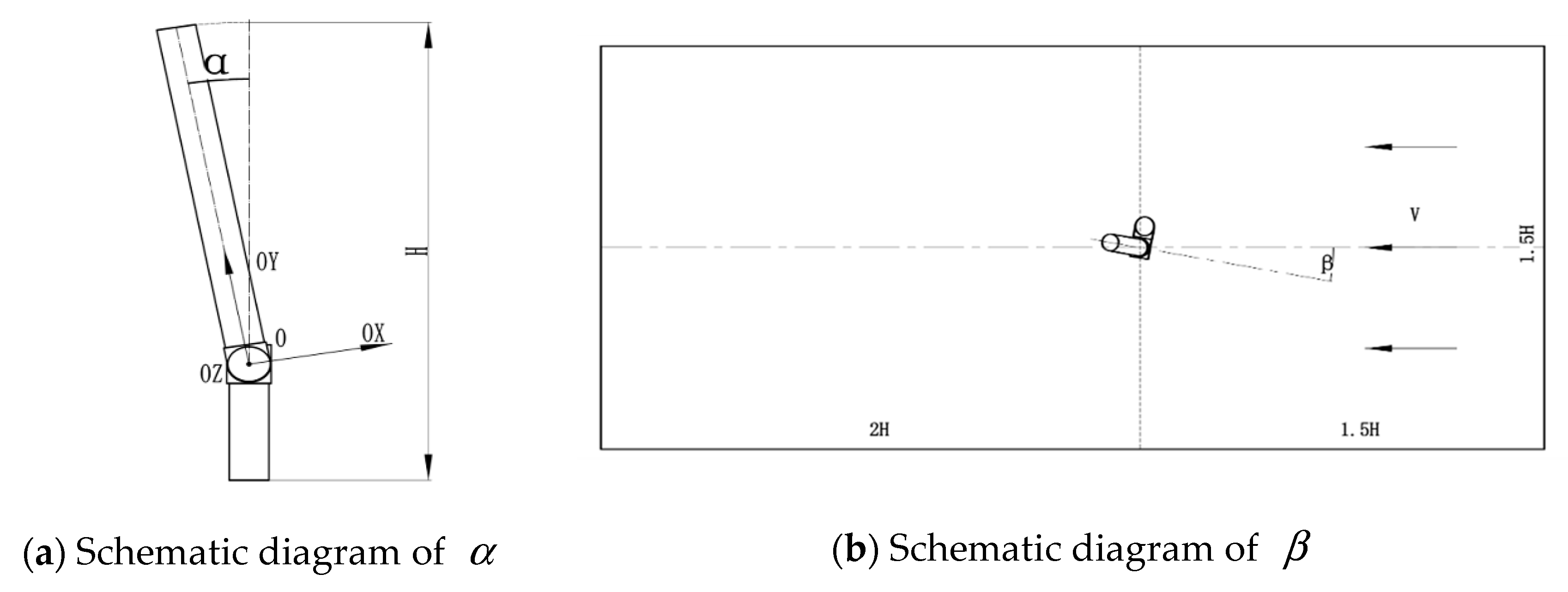
Based on previous experience and multiple numerical practices [6,12,13], this paper establishes the domain as the computational domain, shown in Figure 3b. The specific sizes are as follows:

• Front boundary: 1.5 H
• Back boundary: 2 H
• Side boundary: 1.5 H

where, H stands for the sum of the height of the arm and the base.

The motion parameters of the simulation are shown in Figure 3, α stands for the rotation angle around the OZ axis, β for the angle of the arm to the flow direction, V for the inlet flow velocity of the domain, and the linear velocity components of the manipulator are as shown in Equation (5):

$$\{\begin{array}{l}\mathrm{u}=\mathrm{Vcos}\beta \cos \alpha \\ \mathrm{v}=\mathrm{Vcos}\beta \sin \alpha \\ \mathrm{w}=\mathrm{Vsin}\beta \end{array}$$

(5)

3.2. Meshing

The calculation of CFD requires well-distributed grids. Usually, grids are classified into structured and unstructured grids. The unstructured grid means that internal points in the mesh area do not have the same adjacent unit, with no regular topology, not arranged in layers, and the distribution of mesh nodes is arbitrary. Therefore, it is more flexible than structured grid. Unstructured grids can be optimized by using certain criteria in the process of their generation. Ultimately, they can be displayed as high-quality meshes, which are suitable for complex geometry, easy to control grid size, and node density. Moreover, the adoption of random data structures is conducive to mesh adaptation. It is difficult to model the structured mesh due to the shape of the manipulator, instead, the unstructured mesh is easy to combine with the dynamic mesh technology. Thus, the unstructured mesh is adopted in the research.

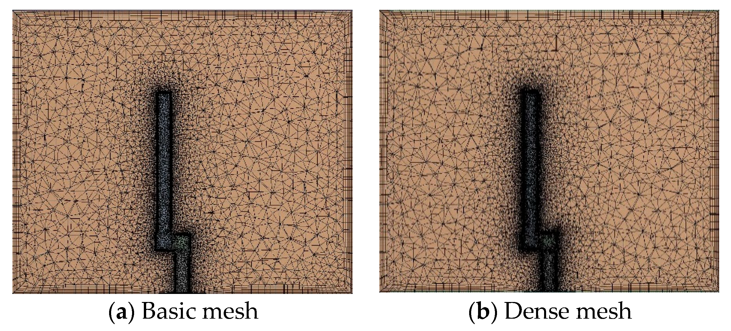
We compare basic mesh to dense mesh for the sake of grid independence verification. Basic mesh in the vicinity of the manipulator is shown in Figure 4a and dense mesh is shown in Figure 4b. The number of elements and nodes are shown in

Table 1. Parameters of basic and dense mesh.

	Maximum Layers	Growth Rate	Elements	Nodes
Basic Mesh	5	1.2	636,457	114,559
Dense Mesh	5	1.2	1,429,231	401,609

.

The rotation process of the manipulator is realized by UDF and dynamic mesh technology in Fluent. Dynamic meshing is performed by using the spring smoothing model, which approximates connecting lines between the grid nodes as springs, and the position of nodes after smoothing is obtained by calculating force equilibrium equations between them. In the calculation process, meshes with a large aberration rate or huge change in size are grouped together to re-divide the partial meshes.

3.3. The Solution of Position Derivatives, Rotation Derivatives, and Coupling Derivatives

Solving the unknown coefficients in Equation (2) is the key to the research task, where Y_v, N_v, Z_w, and M_w are positional derivatives, Y_r and N_r are rotational derivatives, and the remaining unknown coefficients are coupled derivatives.

The positional derivatives could be obtained by simulating the low-speed wind tunnel test, and the rotational derivatives are obtained by measuring the viscous hydrodynamic of the model at different rotational angular velocities. The number of coupled derivatives is large, and the viscous hydrodynamic subjected to the rotational manipulator is measured when β is not 0. After extensive experiments, the viscous hydrodynamic coefficients were obtained by least-square regression analysis.

The calculation domain inlet is set as the velocity boundary, the outlet as the free-flow condition, and the calculation domain wall as the non-slip fixed wall.

According to the research of the turbulence model in the reference [13], the standard k–ω model has many advantages, such as good numerical stability, accurate solution of pressure gradient, low Reynolds number influence, compressibility effect, and shear flow diffusion. It has better adaptability in calculating the flow problem of the boundary layer separation. It is one of the most widely used turbulence models for the viscous hydrodynamic solution. Therefore, the standard k–ω model is used as the turbulence model in this paper. The equation of the kinetic energy k and the turbulent frequency ω are as shown in Equation (6). The determined model parameters are shown in

Table 2. Standard k–ω model parameters.

${\mathit{\sigma }}_{\mathbf{k}}$	${\mathit{\sigma }}_{\mathit{\omega }}$	${\mathit{\alpha }}_{\mathbf{t}}$	${\mathit{\beta }}_{\mathbf{t}}$	${\mathit{\beta }}^{\prime }$
2.0	2.0	5/9	0.075	0.09

, according to the reference [13]:

$$\{\begin{array}{ll}\frac{\partial \rho \mathrm{k}}{\partial \mathrm{t}}+\nabla \cdot (\rho \overrightarrow{\mathrm{U}}\mathrm{k})=& \nabla \cdot \left[(\mu +\frac{{\mu }_{\mathrm{t}}}{{\sigma }_{\mathrm{k}}})\nabla \mathrm{k}\right]\\ & +{\mathrm{P}}_{\mathrm{k}}-{\beta }^{\prime }\rho \mathrm{k}\omega \\ \frac{\partial \rho \omega }{\partial \mathrm{t}}+\nabla \cdot \left(\rho \overrightarrow{\mathrm{U}}\omega \right)=& \nabla \cdot \left[\left(\mu +\frac{{\mu }_{\mathrm{t}}}{{\sigma }_{\omega }}\right)\nabla \omega \right]\\ & +{\alpha }_{\mathrm{t}}\frac{\omega }{\mathrm{k}}{\mathrm{P}}_{\mathrm{k}}-{\beta }_{\mathrm{t}}\rho {\omega }^2\end{array}$$

(6)

4. Result Analysis

Comparing the viscous hydrodynamics of the manipulator measured by adopting the basic and dense mesh, respectively, we conclude that the differences are in the range from 1.7% to 4.3%. The differences are sufficiently low and negligible.

Computations are executed in a 64-bit processor consist of CPU (Intel Core i5-8400 @ 2.80 GHz) and 8 GB accessible memory, and take 37 h with at least 40 iterations per time step.

Using the size of calculation domain set in Section 3.1, the flow velocity of the calculation domain is kept constant, the angle β between the manipulator and the incoming flow direction is adjusted, the viscous hydrodynamics at different angles are calculated, and then the viscous hydrodynamic position derivative is obtained by linear analysis. The position derivative calculation contents are shown in

Table 3. Solving cases of position derivatives.

$\alpha$	0°, ±2°, ±5°, ±7°, ±10°
$\beta$	0°, ±2°, ±4°, ±6°, ±8°, ±10°
$\mathrm{r}$	0 rad/s
$\mathrm{V}$	1 m/s

.

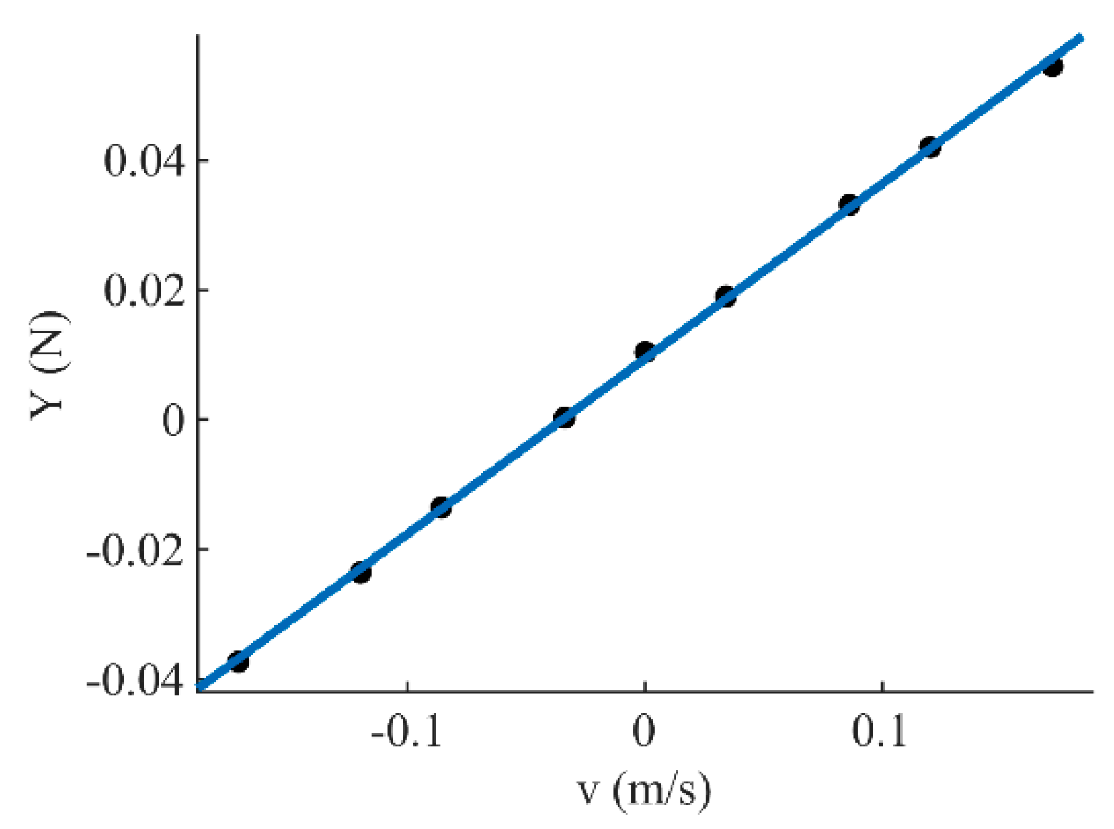
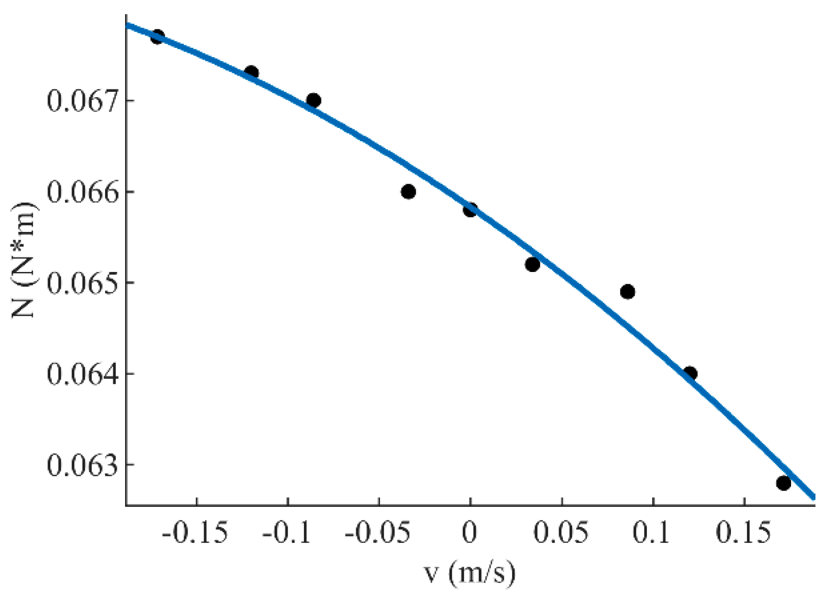
Since the different degrees of α and β cause the manipulator to have different linear velocities in the OX, OY, and OZ directions, viscous hydrodynamics of the arm is measured in the horizontal plane XOZ and the vertical plane XOY, respectively. The values of the vertical force Y and the pitching moment N measured at the different linear velocity v in the OY direction are shown in

Table 4. Measurements of vertical force Y and pitching moment N at different linear velocity v.

v (m/s)	Y (N)	N (N·m)
−0.1714	−0.0373	0.0677
−0.1200	−0.0235	0.0673
−0.0860	−0.0135	0.0670
−0.0340	0.0003	0.0660
0	0.0104	0.0658
0.0340	0.0190	0.0652
0.0860	0.0331	0.0649
0.1200	0.0420	0.0640
0.1714	0.0545	0.0628

.

The position derivatives Yv and Nv are the first derivative coefficients of the linear velocity v, so the least squares curve fitting of the vertical force Y and the pitching moment N in viscous hydrodynamics to the linear velocity v is performed, as shown in Figure 5 and Figure 6. The derivative value at the median 0 points of the line velocity v is taken as the position derivative.

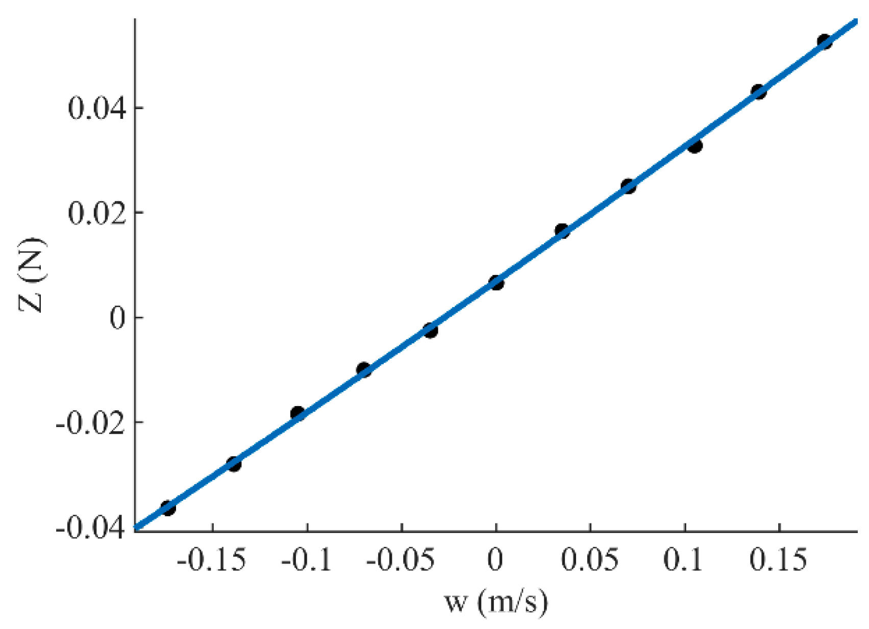
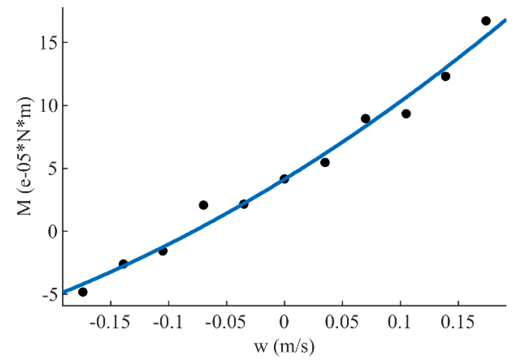
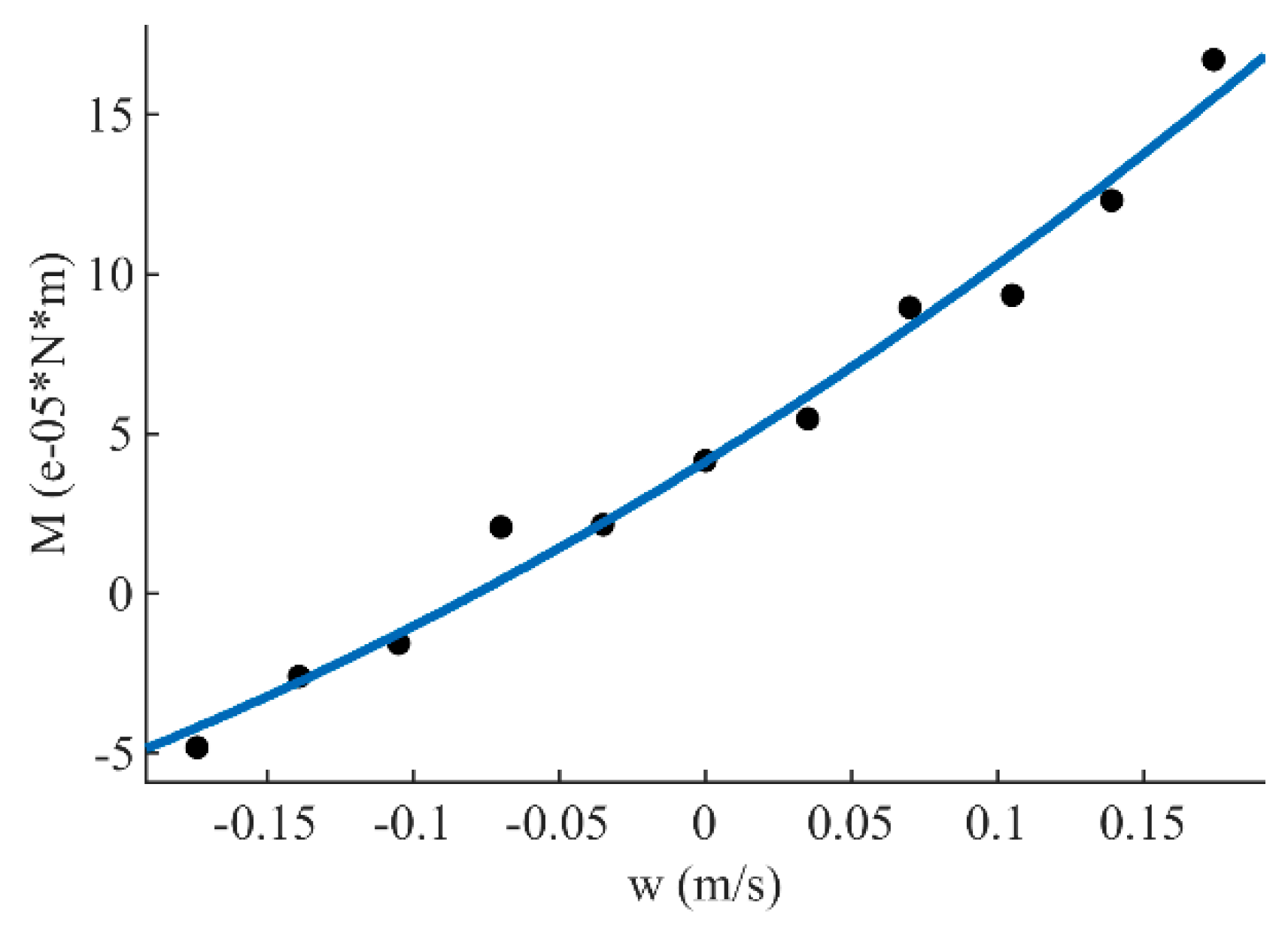
Same as above, the values of the lateral force Z and the yaw moment M measured at the different linear velocity w in the OZ direction are shown in

Table 5. Measurement of the lateral force Z and the yaw moment M at the different linear velocity w.

w (m/s)	Z (N)	M (e−5·N·m)
−0.1740	−0.0364	−4.8199
−0.1390	−0.0280	−2.5920
−0.1050	−0.0184	1.5570
−0.0700	−0.0100	2.0860
−0.0350	−0.0025	2.1628
0	0.0066	4.1640
0.0350	0.0165	5.4699
0.0700	0.0250	8.9650
0.1050	0.0328	9.3461
0.1390	0.0430	12.3140
0.1740	0.0526	16.7242

.

The position derivatives Z_w and M_w are the first derivative coefficients of the linear velocity w, so the least squares curve fitting of the viscous hydrodynamic lateral force Z and the yawing moment M to the linear velocity w is performed, as shown in Figure 7 and Figure 8. The derivative at 0 point of the median line velocity w is taken as the position derivative.

The positional derivatives could be obtained as shown in

Table 6. Position derivatives of the manipulator in viscous hydrodynamics.

${\mathbf{Y}}_{\mathbf{v}}$	${\mathbf{N}}_{\mathbf{v}}$	${\mathbf{Z}}_{\mathbf{w}}$	${\mathbf{M}}_{\mathbf{w}}$
1.4352	−0.1472	1.3520	0.0117

below:

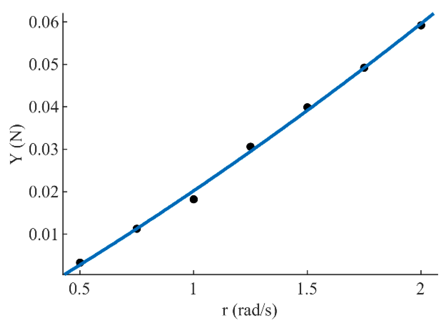
Since the manipulator studied in this paper is a single DOF, only the viscous hydrodynamics are measured when it rotates around the OZ axis. UDF is applied to adjust the rotational velocity of the arm. The measurement conditions of the rotation derivatives are shown in

Table 7. Solving cases of rotational derivatives.

$\alpha$	−10°–10°
$\beta$	0°
r	0.5, 0.75, 1, 1.25, 1.5, 1.75, 2.0 (rad/s)
V	0 m/s

.

This paper calculates the hydrodynamics of the rotating underwater manipulator when the flow is stationary. The arm rotates in the XOY plane. The angular velocity r is adjusted according to Table 7, and the instantaneous viscous hydrodynamics of the arm during the rotation from −10° to 10° around the OZ axis are measured. The measured vertical force Y and pitching moment N are shown in

Table 8. Measurements of vertical force Y and pitching moment N at different angular velocities r.

r (rad/s)	Y (N)	N (N·m)
0.5	0.0033	0.0444
0.75	0.0113	0.0731
1.0	0.0182	0.1023
1.25	0.0306	0.1462
1.5	0.0399	0.1750
1.75	0.0492	0.2181
2.0	0.0592	0.2613

.

The rotational derivatives Y_r and N_r are the first derivative coefficients of the angular velocity r, similar to the solution method of the position derivatives. The least squares curve fitting of the vertical force Y and the pitching moment N in viscous hydrodynamics to the angular velocity r is performed, as shown in Figure 9 and Figure 10. The derivative at the median angular velocity r of 1.25 rad/s is taken as the rotation derivative.

The rotational derivatives could be obtained as shown in

Table 9. Rotation derivatives of the manipulator in viscous hydrodynamics.

${\mathbf{Y}}_{\mathbf{r}}$	${\mathbf{N}}_{\mathbf{r}}$
0.4043	3.0869

below:

The coupled derivative is the second-order viscous hydrodynamic coefficient of the arm under complex motion conditions. Through the transient iterative calculation of the motion of the manipulator at different α and β angles and various angular velocities, the viscous hydrodynamics of each motion state are measured, and many coupling derivatives are obtained by least-squares regression analysis. The coupling derivative solution conditions are shown in

Table 10. Solving cases of coupling derivatives.

$\alpha$	0°, ±2°, ±5°, ±7°, ±10°
$\beta$	0°, ±2°, ±4°, ±6°, ±8°, ±10°
r	0.5 rad/s, 1 rad/s
V	1 m/s

below.

The coupled derivatives are obtained by regression analysis, and the obtained coupled derivatives are processed without dimensioning. The values of the parameters are as shown in

Table 11. Coupling derivatives of the manipulator in viscous hydrodynamics.

${\mathrm{X}}_{\mathrm{uu}}$	−0.6960	${\mathrm{X}}_{\mathrm{vv}}$	−3.8896
${\mathrm{X}}_{\mathrm{ww}}$	−74.4904	${\mathrm{X}}_{\mathrm{rr}}$	44.8128
${\mathrm{X}}_{\mathrm{vr}}$	−275.0688	${\mathrm{Y}}_{\mathrm{v}\left|\mathrm{v}\right|}$	1.172
${\mathrm{Y}}_{\mathrm{r}\left|\mathrm{r}\right|}$	−6.2688	${\mathrm{Y}}_{\mathrm{v}\left|\mathrm{r}\right|}$	31.6064
${\mathrm{Z}}_{\mathrm{w}\left|\mathrm{w}\right|}$	13.0336	${\mathrm{Z}}_{\mathrm{vv}}$	2.1088
${\mathrm{Z}}_{\mathrm{rr}}$	−0.0512	${\mathrm{Z}}_{\mathrm{vr}}$	−0.1264
${\mathrm{K}}_{\mathrm{v}}$	−0.0011	${\mathrm{K}}_{\mathrm{v}\left|\mathrm{v}\right|}$	−0.0160
${\mathrm{K}}_{\mathrm{r}}$	0.1515	${\mathrm{K}}_{\mathrm{r}\left|\mathrm{r}\right|}$	0.0256
${\mathrm{M}}_{\mathrm{w}\left|\mathrm{w}\right|}$	−1.0816	${\mathrm{M}}_{\mathrm{vv}}$	0.0144
${\mathrm{M}}_{\mathrm{rr}}$	0.0384	${\mathrm{M}}_{\mathrm{vr}}$	−0.2144
${\mathrm{N}}_{\mathrm{v}\left|\mathrm{v}\right|}$	32.9184	${\mathrm{N}}_{\mathrm{r}\left|\mathrm{r}\right|}$	−25.0688
${\mathrm{N}}_{\mathrm{v}\left|\mathrm{r}\right|}$	130.4128

.

5. Conclusions

The hydrodynamics of underwater manipulators during operation are complex and difficult to predict. It is analyzed that components of the hydrodynamics include inertial hydrodynamics caused by acceleration and viscous hydrodynamics caused by friction. This paper takes viscous hydrodynamics as the research target.

According to the research on dynamics of AUV (Autonomous Underwater Vehicle), ROV(Remote Operated Vehicle) and ships in other references, the viscous hydrodynamic model of the manipulator is analyzed in the form of Taylor expansion, and the viscous hydrodynamics are measured by using a single-DOF manipulator to simulate the underwater motion, and the viscous hydrodynamic coefficients among the model are calculated via regression analysis. An accurate viscous hydrodynamic model is obtained to predict viscous hydrodynamics of manipulators during operation at any attitude.

This model is the basis for the feedforward control and is helpful to study control stability of underwater manipulators. We believe that although the simulations in this paper were performed for single-DOF manipulators, the modeling method may be extended for the manipulator with multi-DOF and more complicated shapes as is in the case of real underwater manipulators.