Article

Second Path Planning for Unmanned Surface Vehicle Considering the Constraint of Motion Performance

1
Science and Technology on Underwater Vehicle Laboratory, Harbin Engineering University, Harbin 150001, China
2
Beijing Institute of Astronautically Systems Engineering, Beijing 100076, China
*
Authors to whom correspondence should be addressed.
J. Mar. Sci. Eng. 2019, 7(4), 104; https://doi.org/10.3390/jmse7040104
Submission received: 11 March 2019 / Revised: 10 April 2019 / Accepted: 11 April 2019 / Published: 17 April 2019
(This article belongs to the Special Issue Intelligent Marine Robotics Modelling, Simulation and Applications)

Abstract

:
When utilizing the traditional path planning method for unmanned surface vehicles (USVs), ‘planning-failure’ is a common phenomenon caused by the inflection points of large curvatures in the planned path, which exceed the performances of USVs. This paper presents a second path planning method (SPP), which is an initial planning path optimization method based on the geometric relationship of the three-point path. First, to describe the motion performance of a USV in conjunction with the limited test data, a method of integral nonlinear least squares identification is proposed to rapidly obtain the motion constraint of the USV merely by employing a zig zag test. It is different from maneuverability identification, which is performed in combination with various tests. Second, the curvature of the planned path is limited according to the motion performance of the USV based on the traditional path planning, and SPP is proposed to make the maximum curvature radius of the optimized path smaller than the rotation curvature radius of the USV. Finally, based on the ‘Dolphin 1’ prototype USV, comparative simulation experiments were carried out. In the experiment, the path directly obtained by the initial path planning and the path optimized by the SPP method were considered as the tracking target path. The artificial potential field method was used as an example for the initial path planning. The experimental results demonstrate that the tracking accuracy of the USV significantly improved after the path optimization using the SPP method.

1. Introduction

Unmanned surface vehicle (USV), which has attracted significant research attention in recent years, is used for dangerous and inhospitable missions [1,2]. At present, a USV mainly consists of a motion control system [3], sensor system, and communication system.
Path planning [4,5], as the core of USV research, represents the intelligence level of the USV to a certain extent. The path planning method can be used to determine an optimal path from the starting point to the end point, which mainly includes the A* algorithm [6,7,8], genetic algorithm [9], artificial potential field method [10], ant colony algorithm [11], and particle swarm algorithm [12,13]. However, all the abovementioned methods of USV path planning present several drawbacks. The optimal set of path planning is solved based on the shortest distance standard, mostly on the premise that the USV is regarded as a mass point, while ignoring its maneuvering and turning performances. This results in the inability of the underactuated USV to track path nodes with large curvatures beyond the limitations of its own motion performance. In practical engineering applications, planning failures, such as the inaccessibility to the target, the inability to complete the obstacle avoidance task, or detouring, may occur during the trajectory tracking of the USV, thus increasing the difficulty of the tasks.
At present, there are several path planning smoothing methods. For the path planning of a mobile robot, based on the A* algorithm [6,14], all nodes in the planning path are traversed in the grid environment. When there is no obstacle on the connecting line of a node before and after, the intermediate node of the extended line is removed to reduce the number of path turns. However, this method does not consider the maneuverability of the USV in optimization, only the reduction of the number of turns to achieve the optimization effect. For the path planning of an automatic underwater vehicle (AUV), based on the genetic algorithm [15,16], the B spline interpolation method was introduced into the objective function for path smoothing. However, when a few path nodes exceed the turning ability of the AUV, irrespective of the fit between the nodes, the curve formed is unreachable. For the path planning of the USV, based on the statistical method of regression [17], the path smoothing method is dependent on a large amount of actual navigation data, and it is based on an improved A* algorithm (FAA*) [18], to achieve path smoothing. This method limits the initial heading angle of the USV and removes the acute angle section in the planned path. For the path planning of a high-speed numerical control machine, the hyperboloid sheet method is used to solve the path smoothing problem of the continuous path, combined with a straight line and arc [19,20]. However, this method is used to perform curve fitting on planned path points, and the slice of the high-speed cutting machine is more flexible and demonstrates good maneuverability.
Although the abovementioned methods are beneficial to the smooth processing of path planning to a certain extent, in the application of USVs, the methods demonstrated poor adaptability, and the results were accidental. In this paper, using the zig zag test, a rapid and one-time identification and analysis method for the motion performance of the USV is proposed. A second path planning (SPP) method is then proposed to consider the constraints of the USV performance. This method can realize the re-optimization based on the existing path planning method to obtain the optimal path within the range of the motion ability of the USV, and to effectively prevent the occurrence of planning failure. Finally, using the improved artificial potential field path planning method [21] as an example, a second optimization strategy was introduced and applied to the ‘Dolphin 1’ mini-type USV. Moreover, a simulation comparison test was carried out to verify the feasibility and effectiveness of the method.

2. Analyzing the Motion Performance of USV

When the traditional path planning method is combined with the trajectory tracking guidance algorithm of the USV, the planning failure phenomena occur, such as detouring and collision, given that this method considers the USV as a mass point, which is an ideal state. Therefore, in the process of the path planning of the USV, the motion ability of the USV, especially the minimum radius of the turning circle, should be considered.

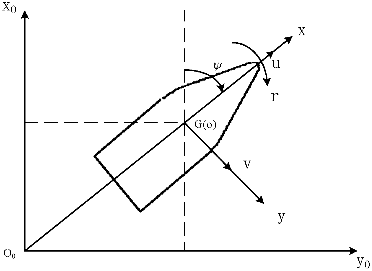
2.1. Modeling the USV Maneuverability

To describe the motion of the USV, two right-handed rectangular coordinate systems were adopted [22]. The first is the inertial frame, o 0 - x 0 y 0 z 0 , and the second is the body-coordinate system, o - x y z (Figure 1). The inertial frame was fixed on the earth. The plane, o 0 - x 0 y 0 , was on the undisturbed free surface, and the axis, x 0 , was directed forward to the initial straight course of the USV with the axis, z 0 , directed downward. The body-coordinate system was fixed on the vehicle, and the origin was located in the middle of it. The plane, o - x y , was on the undisturbed free surface, the axis, x , was in the direction of the bow, the axis, y , was in the direction of the starboard, and the axis, z , was directed downward.
The USV motion equation of six degrees of freedom can be expressed as follows:
{ m ( u ˙ + q w r v ) = X m ( v ˙ + r u p w ) = Y m ( w ˙ + p v q u ) = Z I x p ˙ + ( I z I y ) q r = L I y q ˙ + ( I x I z ) r p = M I z r ˙ + ( I y I x ) p q = N
where the first three equations are the expressions of the motion theorem of the mass center in the body coordinate system, and the last three equations are the Euler dynamics equations of the rotation of a rigid body around a fixed point.
Only considering the horizontal motion, p = q = w = 0 , the linear Equation (2) of the vehicular heading response can be obtained through the transformation of Equation (1):
T 1 T 2 r ¨ + ( T 1 + T 2 ) r ˙ + r = K δ + K T δ δ
In 1957, Nomoto [23] suggested that the first order linear differential equation can be approximately substituted for the second order equation, in the case wherein steering is infrequent, as shown in Equation (3):
T r ˙ + r = K δ
The first order nonlinear Equation (4) is obtained by adding the nonlinear term to the motion of the large rudder angle, low speed, and the study of small ships:
T r ˙ + r + α r 3 = K δ
The mini-type USV evaluated in this study uses two electric propellers as the power device, with a maximum voltage of 12 V. Different voltage values correspond to different speed values. In combination with the model of thrust and velocity in [24], and with reference to the rudder and heading model, the corresponding relationship between the speed and voltage of the USV was established. The speed model of the USV can be expressed as follows:
u = k 1 n 2 + k 2 n + k 3
where u is the longitudinal speed of the USV, n is the propeller voltage, and k 1 , k 2 , k 3 represent the system parameters. The transverse speed can be neglected due to the low speed of the USV evaluated in this study.
In summary, the maneuverability model of the USV can be expressed as follows:
{ x ˙ = u cos ψ v sin ψ y ˙ = u sin ψ + v cos ψ ψ ˙ = r r ˙ = 1 T ( K δ r α r 3 ) u = k 1 n 2 + k 2 n + k 3

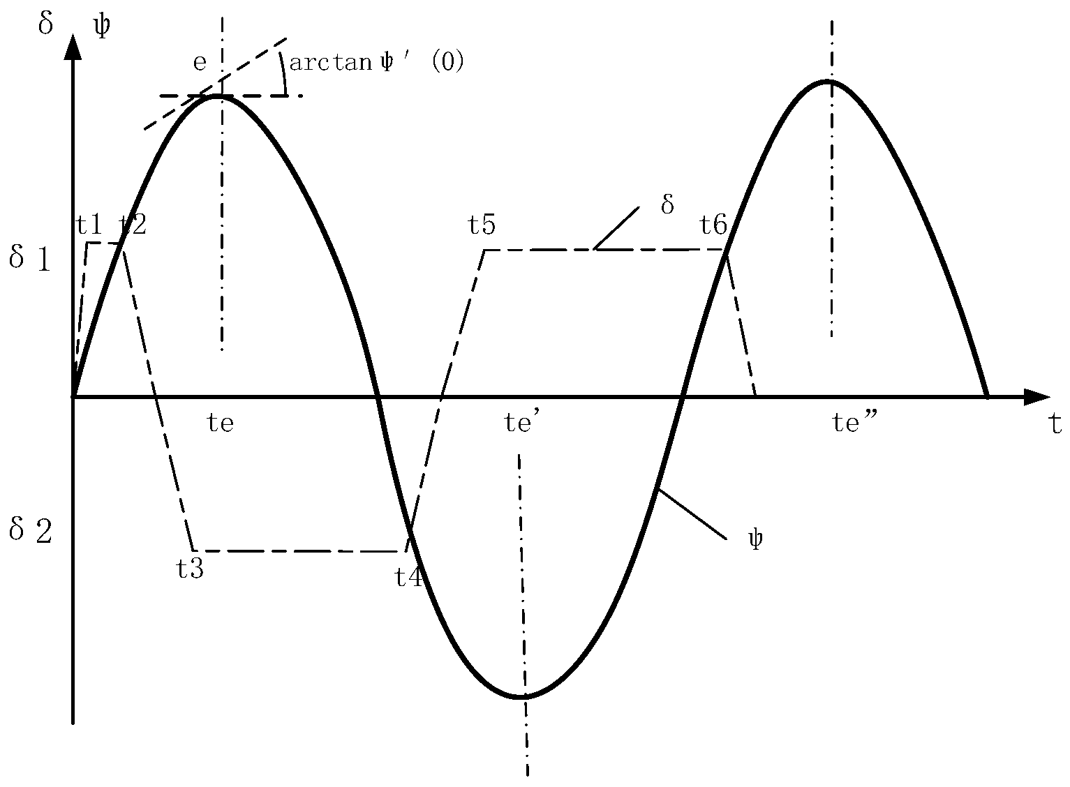
2.2. Integral Nonlinear Least Squares Method

The least squares method [25] is one of the most commonly used motion parameter identification methods. However, this method was typically used to identify the nonlinear motion equation by a combination of experiments, i.e., the zig zag test and the turning circle test. In this paper, an integral nonlinear least squares method is proposed. The nonlinear parameters of the motion equation are transformed and processed. Using a set of zig zag test data, the nonlinear motion equation can be rapidly identified. Based on the identification results, the course control parameters can be predicted, and the motion ability can be analyzed.
Based on the ‘Dolphin 1’ prototype USV, the integral nonlinear least square method was adopted to identify the parameters of the first-order nonlinear control model using the zig zag test data. According to the identified parameters, the corresponding zig zag test manipulation simulation model was established using MATLAB, and the reliability of the method was confirmed by the error between the simulation and actual case. The experimental data were derived from the zig zag test in the Songhua River in Harbin, Heilongjiang, China. Figure 2 presents the layout of the ‘Dolphin 1’ in the Songhua River, and the test data are shown in Figure 3. The ‘Dolphin 1’ is a mini unmanned catamaran with a single floating body length of 2.0 m, diameter of 0.25 m, and a two floating body spacing of 1.1 m. It is propelled by two propellers with a rear-mounted rudder plate, and the maximum speed is 1.2 m/s.
At 10.0 volts, the ‘Dolphin 1’ carried out the zig zag test control experiment at a speed of 1.08 m/s. The variation curve of the heading and rudder angle with respect to time is shown in Figure 3.
According to the test, the first order nonlinear K-T Equation (6) was identified using integral nonlinear least squares. Referring to Figure 4, given that the vehicle has no real-time measurement record of angular acceleration, the integral of both sides of Equation (6) was carried out based on the time region, [a,b]. By means of the integral, the angular acceleration was eliminated, and the heading angle data was introduced to identify the mini-type USV maneuvering model:
T a b r ˙ d t + a b r d t + α a b r 3 d t = K a b δ m d t
According to the actual field test data, the operating tempo of the program of the USV control system was 0.15 s. Hence, the N equal interval was adopted, and the equal spacing value was 0.15. For the i-th interval, the linear terms were integrated and then discrete:
{ a i = a i δ m ( t ) d t b i = [ φ ˙ ( i ) φ ˙ ( a ) ] = [ r ( i ) r ( a ) ] θ i = φ ( i ) φ ( a )
For the nonlinear term, c i = a i r 3 d t , given that r is a function of t, the integral of r 3 ( t ) with respect to the time, t, is complex and difficult to solve. When the experimental data is discrete, the Newton-Cotes quadrature equation is adopted to calculate the product, as shown in Equation (9).
Definition 1.
[26] Integrand, f ( x ) [ a , b ] , given a set of nodes, a x 0 < x 1 < < x n b , and given the value of the function, f ( x ) , on these nodes, the Lagrangian interpolation polynomial, L n ( x ) , is applied; thus:
I n ( f ) = a b f ( x ) d x a b L n ( x ) d x = a b [ k = 0 n l k ( x ) f ( x h ) ] d x = k = 0 n f ( x k ) a b l k ( x ) d x = k = 0 n A k f ( x k )
where A k = a b l k ( x ) d x . Equation (9) is referred to as the interpolation formula. The remainder of the interpolation formula is shown in Equation (10):
E ( f ) = a b [ f ( x ) L n ( x ) ] d x = a b R n ( x ) d x = a b f ( n + 1 ) ( ζ ) ( n + 1 ) ! ω n + 1 ( x ) d x
where ζ ( x 0 , x n ) is dependent on x . ω n + 1 ( x ) = ( x x 0 ) ( x x 1 ) ( x x n ) .
The quadrature coefficient, A k , is independent of f ( x ) , and it is related to the equidistant nodes, x k , and integral interval, [ a , b ] . The integral formula of the Newton-Cotes (11) can be obtained by transforming A k :
I n ( f ) = ( b a ) k = 0 n C k ( n ) f ( x k )
C k ( n ) = ( 1 ) n k n k ! ( n k ) ! 0 n t ( t 1 ) ( t k + 1 ) ( t k 1 ) ( t n ) d t
where C k ( n ) is referred to as the cotes coefficient. The coefficient of cotes is shown in Table 1.
Based on the actual test data, h = 0.15 , the method takes n = 1.0 , divides the interval, [ a , i ] , into m equal parts, counts c = 1.0 , and uses a composite integral formula to reduce the remaining terms.
According to Equation (10), the remainder of the composite newton-cotes interpolation can be obtained:
E f = k = 0 m 1 [ h 3 12 f ¨ ( ζ k ) ] h 2 12 [ f ˙ ( i ) f ˙ ( a ) ]
When n = 1.0 , the composite function, g ( x ) = r 3 ( x ) , can be considered as g ( r ) = r 3 . Moreover, by considering the concavity and convexity of the function, the right side of the equation is divided into two parts in the process of the composite Newton-Cotes quadrature, i.e., the exact solution and the approximate solution. In addition, the gain coefficient is introduced to reduce the interpolation remainder, and c i is shown in Equation (14):
c i = a i r 3 ( t ) d t = α 1 2 ( r 3 ( i ) r 3 ( a ) ) Δ t + r 3 ( a ) Δ t
where α = 0.5 .
Utilizing the least square method, the left and right sides of Equation (15) are respectively considered as functions, and the square of their difference can be minimized to obtain the values of K , T , α :
J = i = 1 N ( K a i + T b i + α c i θ i ) 2
{ J K = 0 2 ( K a i 2 + T b i a i + α c i a i θ i a i ) = 0 J T = 0 2 ( K a i b i + T b i 2 + α c i b i θ i b i ) = 0 J α = 0 2 ( K a i c i + T b i c i + α c i 2 θ i c i ) = 0
The same method can also be used to solve the parameters of the velocity model.

2.3. Identification of Maneuverability and Analysis of Motion Ability

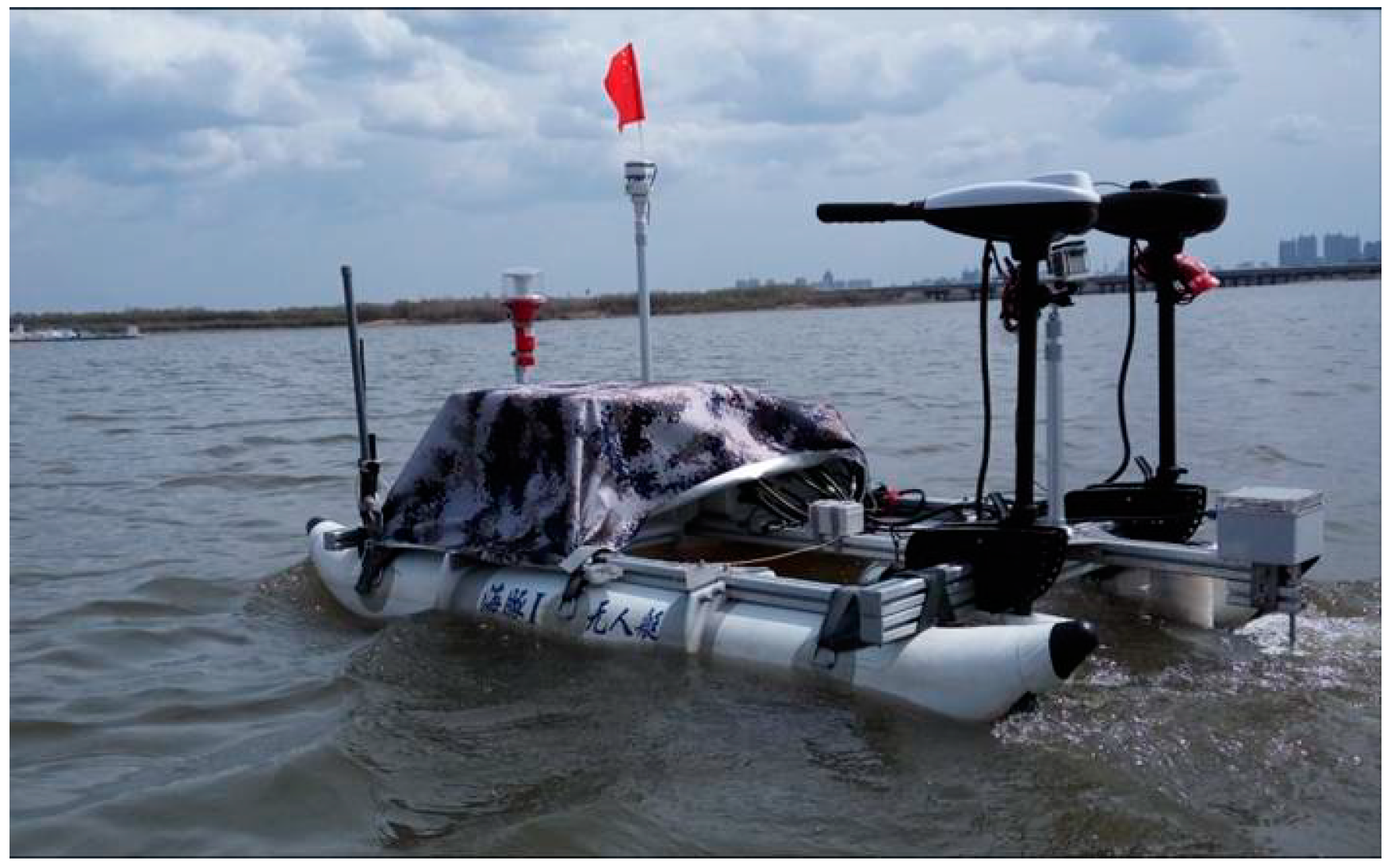
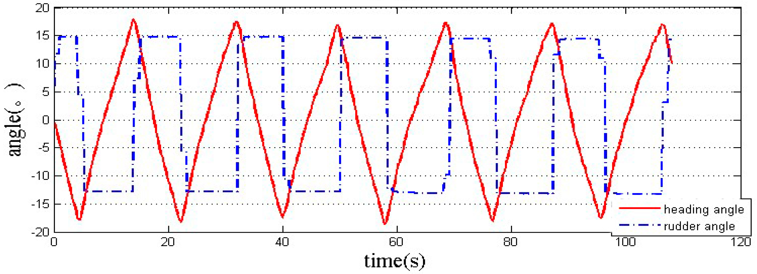
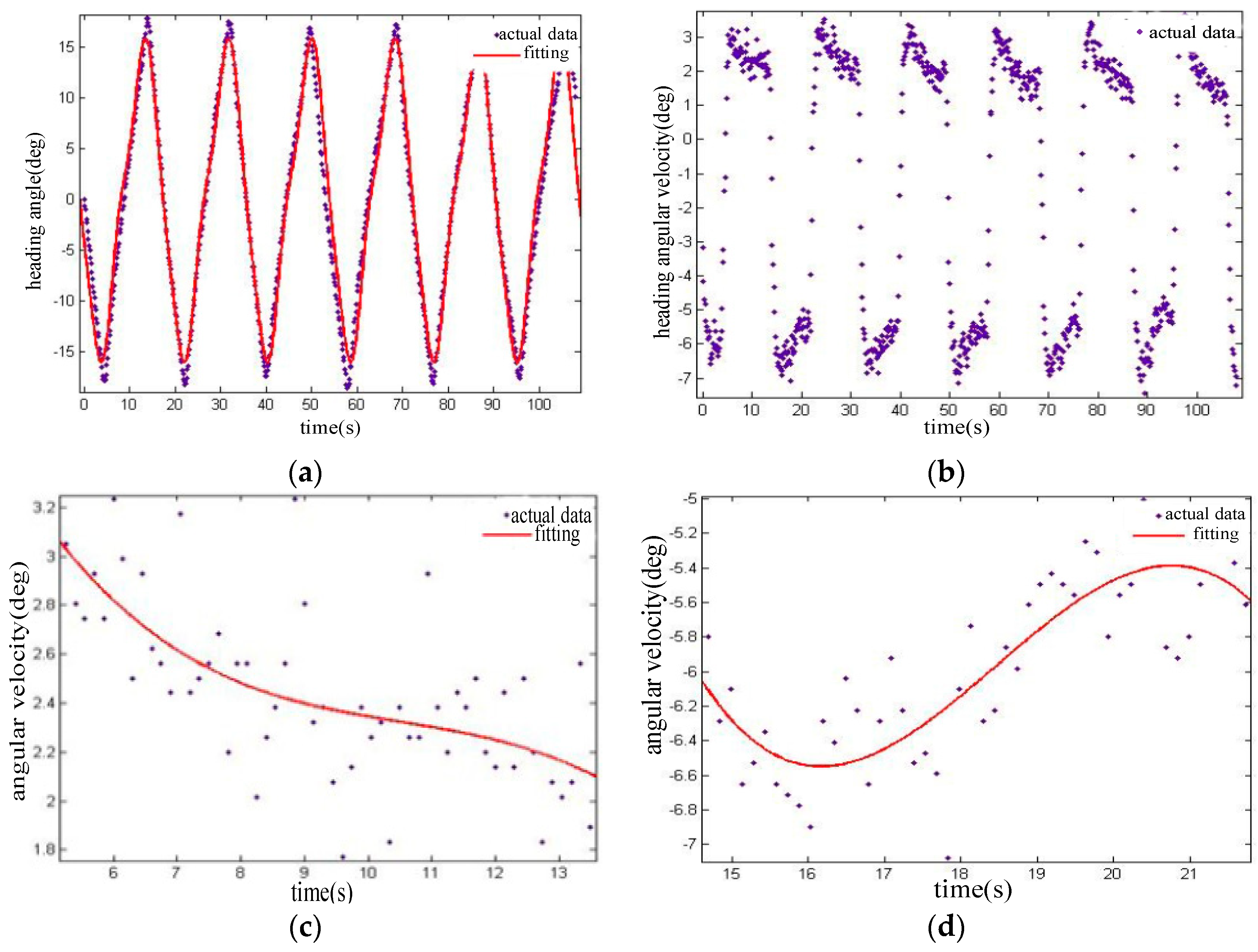
2.3.1. Identification of USV Maneuverability by Field Test Data

Given that the data from the zig zag test conducted in the Songhua River had wild values, the outliers were primarily deleted by data fitting. The curve fitting heading angle was a 7th order Fourier function [27], and the curve fitting heading angular velocity was the piecewise cubic polynomial function. The fitting curves of the heading angle and heading angular velocity are shown in Figure 5a–d.
According to the fitting curve, the wild values (data points with large deviation) were eliminated. { K = 0.286642 T = 0.410205 α = 0.008477 , as obtained from Equation (16). A zig zag test manipulation experimental simulation model was established in MATLAB. Based on the solved values of K , T , α , the predicted heading angle obtained by the simulation under the same rudder angle input was compared with the actual test data. The results are presented in Figure 6 and Figure 7.
According to Figure 7, at the same input rudder angle, the heading angle error was in the ± 5 ° interval. Considering the communication delay, inertia of the USV, accuracy of the rudder angle feedback, and that of the heading angle sensor, the fitting curve was consistent with the actual data.
Based on the velocity and voltage data, the least squares identification method was used to obtain k 1 = −0.006, k 2 = 0.159, and k 3 = 0.004. The comparison results are presented in Figure 8 and Figure 9.

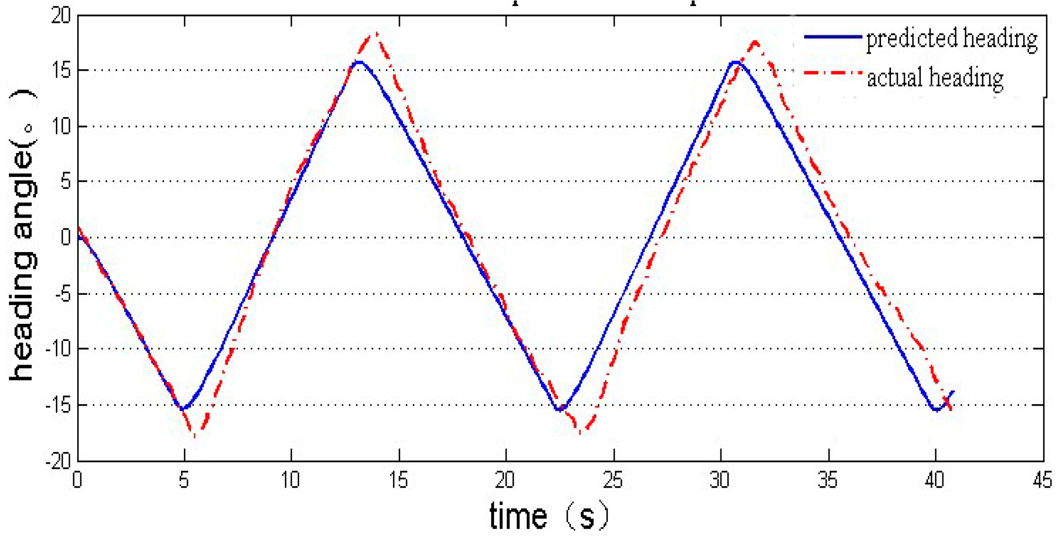
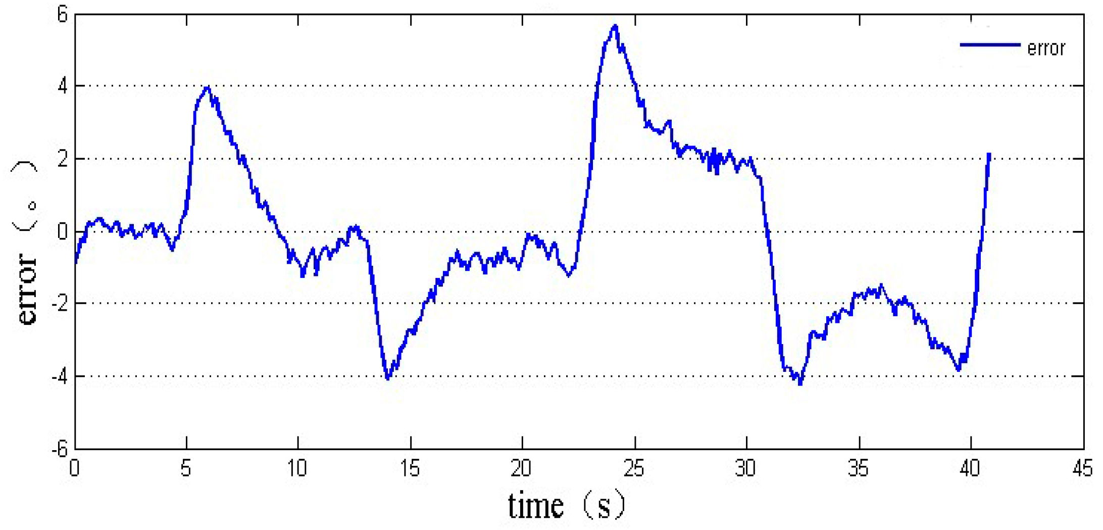
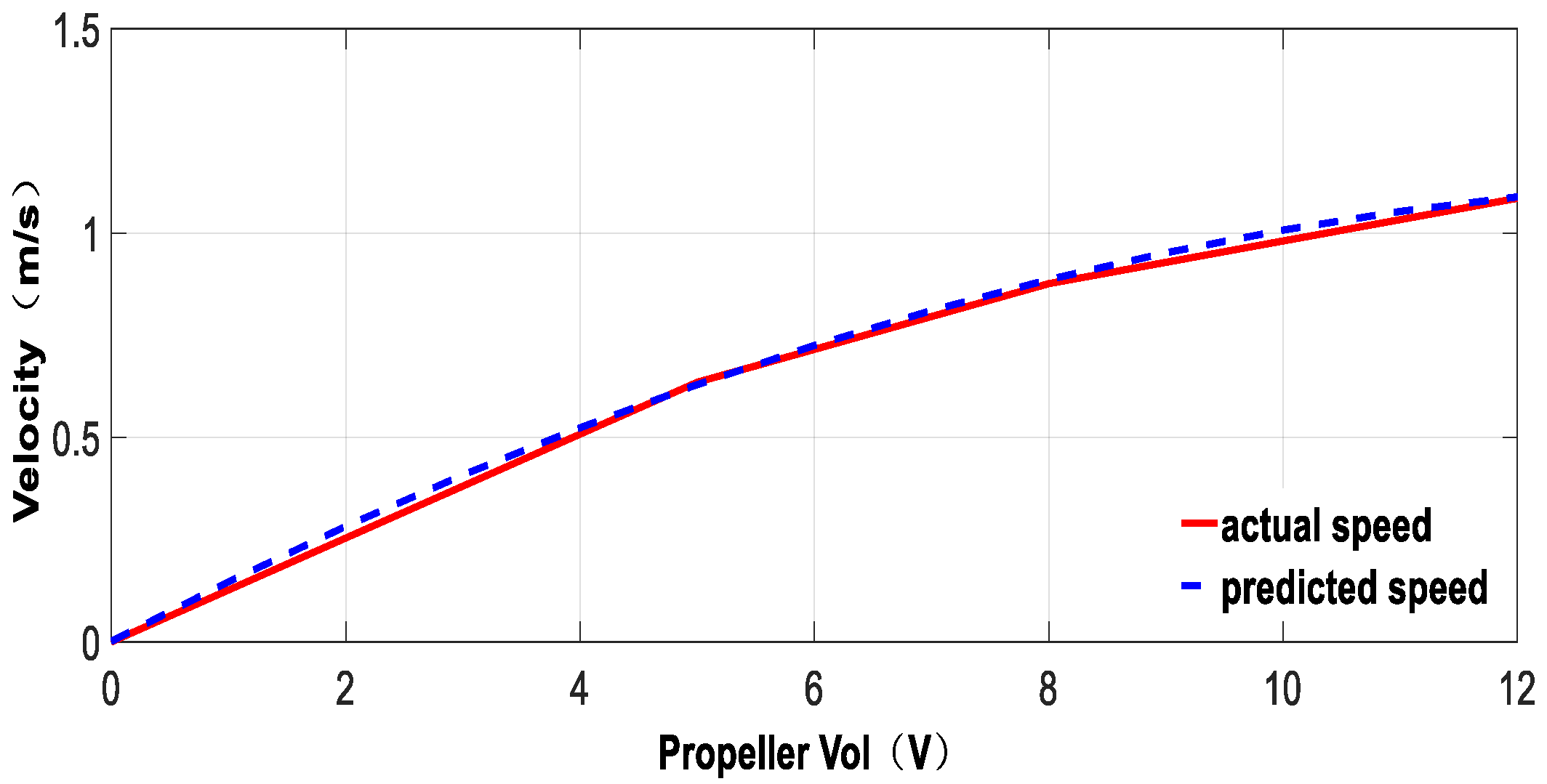
2.3.2. Simulation and Analysis of USV Motion

When the USV is sailing in a straight line, the vehicle deviates from the original route and makes a turning movement at a certain rudder angle. The radius of the circle formed by the trajectory of the USV center of gravity is referred to as the radius of steady rotation. K is the constant rotation angular velocity due to the unit rudder angle, which is directly proportional to the radius of rotation, and inversely proportional to the curvature of steady rotation. Therefore, the maximum rotational curvature can be considered as an evaluation index of the USV motion ability.
Using Equation (16), the dynamic model of the ‘Dolphin 1’ USV was solved, and the turning circle simulation model was established based on MATALB software. Moreover, a proportional–integral–derivative (PID) control method was adopted to establish the control law [28], as shown in Equation (17):
u = K p e + K i e d t + K d d e d t
where u is the output of the controller, and e is the deviation between the given expected value and the actual output value. The simulated steady rotation trajectory is presented in Figure 10. The initial position coordinate of the USV was (0,0), the rudder angle was constant at 30.0°, and the iterative step length and control cycle were 0.15 s.
To confirm the reliability of the motion analysis, the field steady turning test data of ‘Dolphin 1′ were used for comparison. The data were collected and recorded at a rudder angle with a fixed value of 30.0°. The trajectory of the USV is shown in Figure 11.
In Figure 11, the distance between two course path points at A(126.53852,45.79677) and B(126.53851,45.79691) were calculated. Using Equation (18), the longitude and latitude coordinates can be converted from angular units to metric units:
R t u r = π 360 ( A l o n B l o n ) 2 + ( A l a t B l a t ) 2 R g l o b l e
where R g l o b l e = 6371.393 km is the radius of the earth, and the radius, R t u r , of ‘Dolphin 1’ is 7.8 m. By analyzing and comparing Figure 10 and Figure 11, the two turning trajectories were found to be identical.
The integral nonlinear least square method was employed to analyze and determine the performance index of the USV, which was found to demonstrate a high efficiency, convenience, and high accuracy.

3. SPP of USV

In this paper, a second path planning method (SPP) is presented, which is not restricted by the USV motion ability. The improved artificial potential field method proposed by Huang Xinghua [21] was selected as the first path planning method in this study. On the premise of the existing planning path, the second path optimization was carried out to calculate an optimal path constrained by the motion performance of the vehicle. This method was used to solve the problem and deficiency of the traditional USV path planning.

3.1. SPP Model

The SPP of the USV refers to the optimal path constrained by the performance of the USV, which was selected according to the existing optimal path and the three-point geometric relationship. This method preserves the preferred criteria of the traditional path planning.
The SPP model can be described as follows.
Assuming that x , y are the coordinates in the inertial coordinate system, and p i = [ x i , y i ] T is defined as the coordinate position of a path point, the set of n path points derived from the traditional path planning can be expressed as p = [ p 1 T p n T ] T . The check point at time k can be expressed as p k = [ x k , y k ] T , and ϖ is the second planning task variable. The task function is established by combining the geometric constraint relationship of the path, and the corresponding task function can be expressed as shown in Equation (19):
ϖ = f ( p k 1 , p k , p k + 1 )
{ ( ϖ ϖ d ) < 0 , { p k 1 = p k p k = p k + 1 ( ϖ ϖ d ) 0 , { p k = p k + 1 p k + 1 = p k + 2
where ϖ d is the constraint index variable of the motion performance of the vehicle. When ( ϖ ϖ d ) < 0 , the current check point is maintained and the next path point is discussed. When ( ϖ ϖ d ) 0 , the current checkpoint is discarded and the next point of the optimal set of paths is tested until the checkpoint is the endpoint of the path. The schematic diagram of SPP is shown in Figure 12.
The second path planning is applicable to the traditional USV path planning method, which can be used to solve a series of discrete path point sets.
Using the improved artificial potential field method proposed by Huang Xinghua [21] as an example, as shown below, the path planning of the USV involved the implementation of the secondary optimization subject to its motion constraint.

3.2. An Improved Path Planning for the Artificial Potential Field Method

The artificial potential field method (APF), initially proposed by Khatib, was applied to the obstacle avoidance motion planning of a robot manipulator, which had as its objective the realization of the real-time obstacle avoidance of a mechanical arm. The essence of the APF is to define an abstract potential field artificially for the operating space of the robot, which is the superposition of the gravitational field of the target position and the repulsive force field of the obstacle in the environment. The negative gradient of the force field is the virtual force that acts on the robot, and the resultant force of gravity and repulsion represent the accelerating force of the robot.
Although the path planned by the artificial potential field method is efficient, smooth, and safe, there are several drawbacks related to this method [29,30,31,32,33,34], i.e., (1) the local minimum problem; (2) the inability to navigate through closely-situated obstacles; and (3) oscillations near the obstacle. The main objective of the improved artificial potential field method [21] proposed by Huang Xinghua is the solution of these problems to establish a new potential field function. Hence, during the approach of the target point by the robot, the repulsion field is close to zero and the position of the robot target point is the minimum point of the entire situation field; thus, the target can be reached. The repulsion force potential field function of the improved artificial potential field method can be expressed as shown in Equation (21):
U r e p ( X ) = { 1 2 k r e p ( 1 X X o 1 ρ 0 ) 2 ( X X g ) n ( X X o ) ρ 0 0 ( X X o ) ρ 0
where 0 ≤ n < 1.
The negative gradient of the potential field function is also considered as the corrected repulsive force of the repulsion field, as follows:
F r e p ( X ) = U r e p ( X ) = { F r e p 1 + F r e p 2 ( X X o ) r o 0 ( X X o ) > r o
where:
F r e p 1 = k r e p ( 1 X X o 1 ρ o ) 1 ( X X o ) 2 ( X X o ) X ( X X g ) n
F r e p 2 = 1 2 k r e p ( 1 X X o 1 ρ o ) 2 ( X X g ) n X
where U r e p is the repulsive field of the obstacle, ρ is the distance between the robot and the obstacle, ρ 0 is the maximum influencing range of the obstacle, k r e p is the constant of the repulsive field, n is positive, X represents the coordinates of the robot, X g represents the coordinates of the target point, and represents the sign of the gradient.
The gravitational potential field function can be expressed as follows:
U a t t ( X ) = 1 2 k ( X X g ) 2
where U a t t is the gravitational field generated by the target point, and k is the gain constant. Gravity can be expressed as shown in Equation (26):
F a t t ( X ) = U a t t ( X ) = k ( X g X )

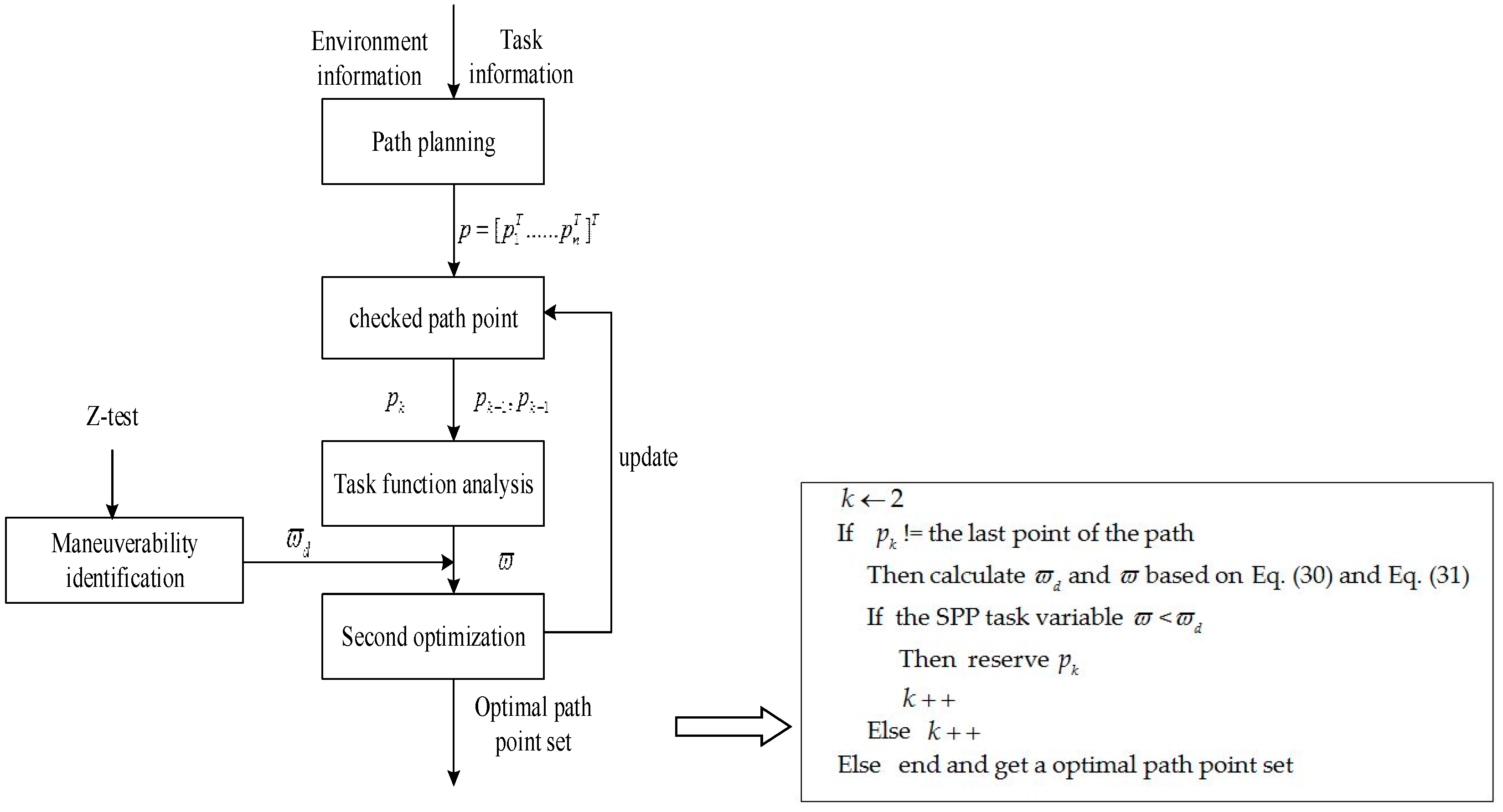
3.3. SPP of the Improved Artificial Potential Field Method

Combined with the improved artificial potential field method, the theoretical block diagram of the second path planning constrained by the motion of the USV is shown in Figure 13.
When the vehicle is performing the navigation task, the starting position, target position, and obstacle position are determined according to the mission information and sea chart information. According to the objective function of the artificial potential field method, a set of path points are obtained. The starting position is reserved, and the second planning task function is analyzed from the second point, as shown in Equation (27):
D k = p k p k 1 D k + 1 = p k + 1 p k D k 1 = p k 1 p k + 1
D ˜ = i = 0 2 D k 1 + i
J k = 1 2 [ D ˜ ( D ˜ 2 D k ) ( D ˜ 2 D k 1 ) ( D ˜ 2 D k + 1 ) ] 1 2
where p k represents the location coordinates of the path point that correspond to the current check moment, k ; p k + 1 , p k 1 are the path points of the current test point forward and backward once, respectively; D i is the distance of the two path points; D ˜ is the distance between the path points; and J k is the size of the region across the three path points. The second planning task variable can be expressed as follows:
ϖ = f ( p k 1 , p k , p k + 1 ) = 4 J k D k D k 1 D k + 1
ϖ d = 1 r
where ϖ d is the constraint index variable of the USV motion performance, and its value can be determined by the rotational curvature of the vehicle. Substituting Equations (30) and (31) into Equation (19), the second optimization can be evaluated.

4. Simulation Test of Trajectory Tracking of USV by SPP Method

Considering the ‘Dolphin 1’ mini-type USV as the test object and using the improved artificial potential field method proposed by Huang Xinghua [21] as an example, the path planning optimization method presented in this paper was simulated and verified. The simulation platform was developed using MATLAB software, the PID control method was employed to control the course and speed, and the trajectory tracking method was implemented in conjunction with the PP method.

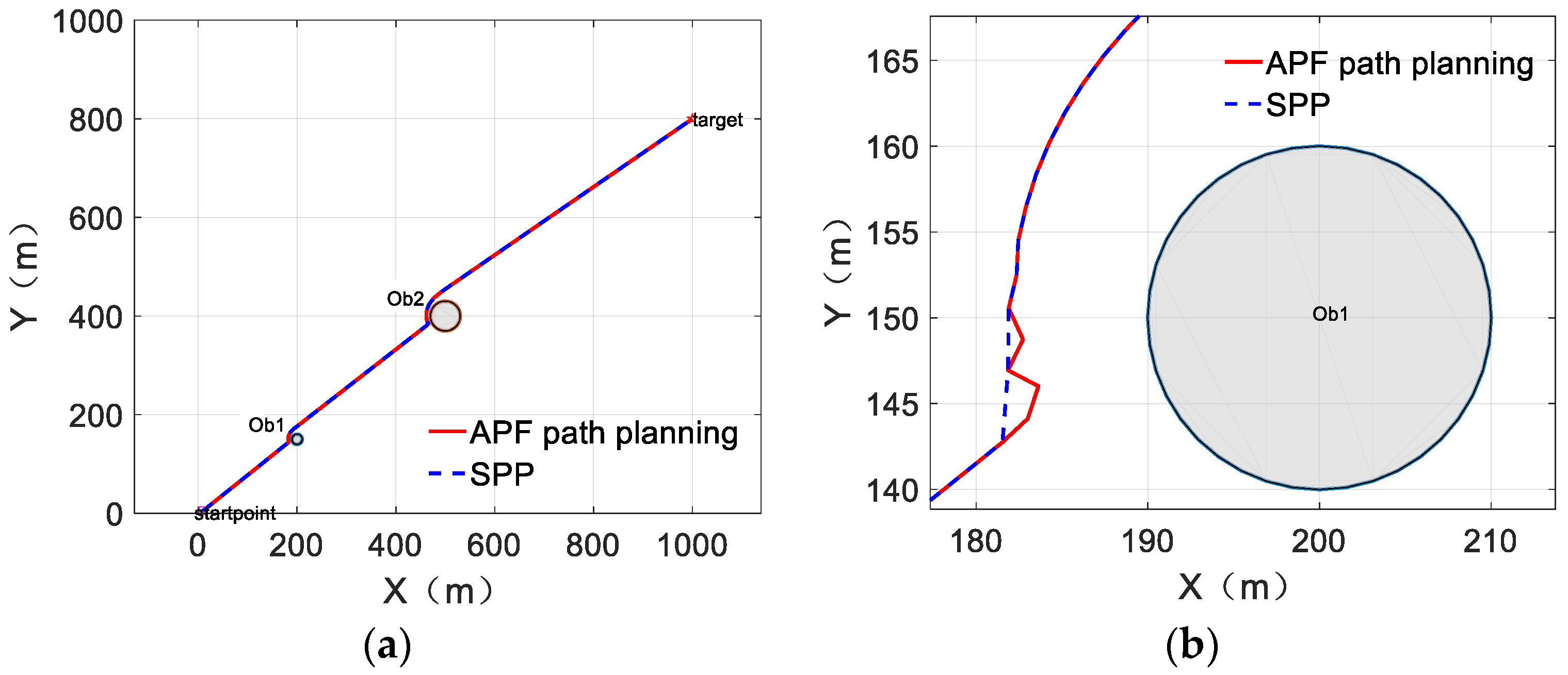
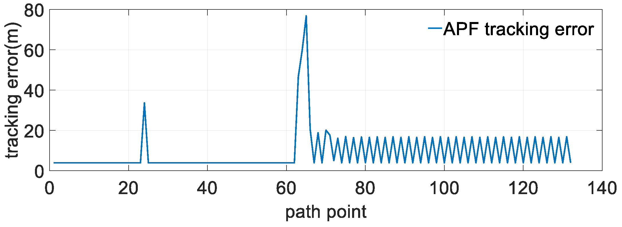
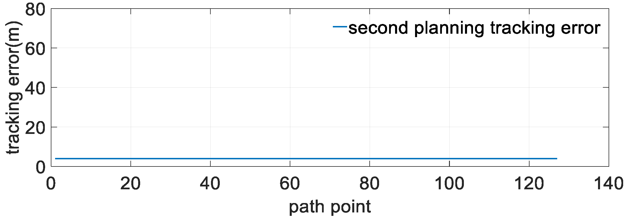
4.1. Comparative Experiment of Small Planning Step

The initial position of the USV was (10 m, 5 m), the target position was (1000 m, 800 m), the length of the vehicle was l = 2.0 m, and the planning step, t p , was t p = 2.0 m. The locations of the obstacles were (200 m, 150 m) and (500 m, 400 m), respectively. The radius of the obstacles, r , corresponded to 10.0 m and 30.0 m, and the influencing radius was defined as r _ i n = r + t p / l l , where   is the integer sign considered upward.
The results of the comparison between the initial path planning using the improved artificial potential field method and the second path planning under the consideration of the motion performance of the USV are shown in Figure 14a. Figure 14b presents the local magnification of the path planning near the first obstacle. In Figure 14a, the solid line represents the initial planning path, and the dotted line represents the optimized path by the secondary planning. The figure illustrates that the initial planning path near the obstacle produces zig-zag oscillations, and the intensity of the path oscillation is related to the impact of the obstacle on the connectivity of the starting point and the end point, in addition to the size of the obstacle. As shown in Figure 14b, given that the SPP method is optimized based on the initial path; it retains the fitness function standard of the initial planning and reduces the oscillation of the initial planning path through optimization.
On the Simulink simulation platform, a USV motion model was developed. The iterative step length and control cycle were 0.15 s. The parameters of the course PID controller were set as p = 1.0 , i = 0.001 , d = 1.0 , the parameters of the speed controller were p = 2.0 , i = 0.001 , d = 0.001 , and the trajectory tracking adopted the pure tracking (PP) method [35,36,37]. In the simulation experiment, when the time exceeded 50.0 s, the target point was replaced, although the vehicle had not reached the distance threshold of the target in the current tracking stage. The simulation results of the USV trajectory tracking of the two methods are respectively shown in Figure 15a,c. The tracking deviation of the two methods is shown in Figure 15b,d.
As can be seen from Figure 15a,c, under the premise of a small planning step length, t p = 2.0 m, the vehicle can track the optimized path after the initial planning using an artificial potential field method and secondary planning method, respectively, and successfully complete the obstacle avoidance task. The comparison and analysis of Figure 15b,d illustrate that although both methods can be used to achieve obstacle avoidance and complete the tracking tasks by SPP, the actual course path of the vehicle was more consistent with the planned path than by APF. This is because secondary programming is an optimization standard of the maneuverability of the USV, which leads to a higher tracking accuracy.

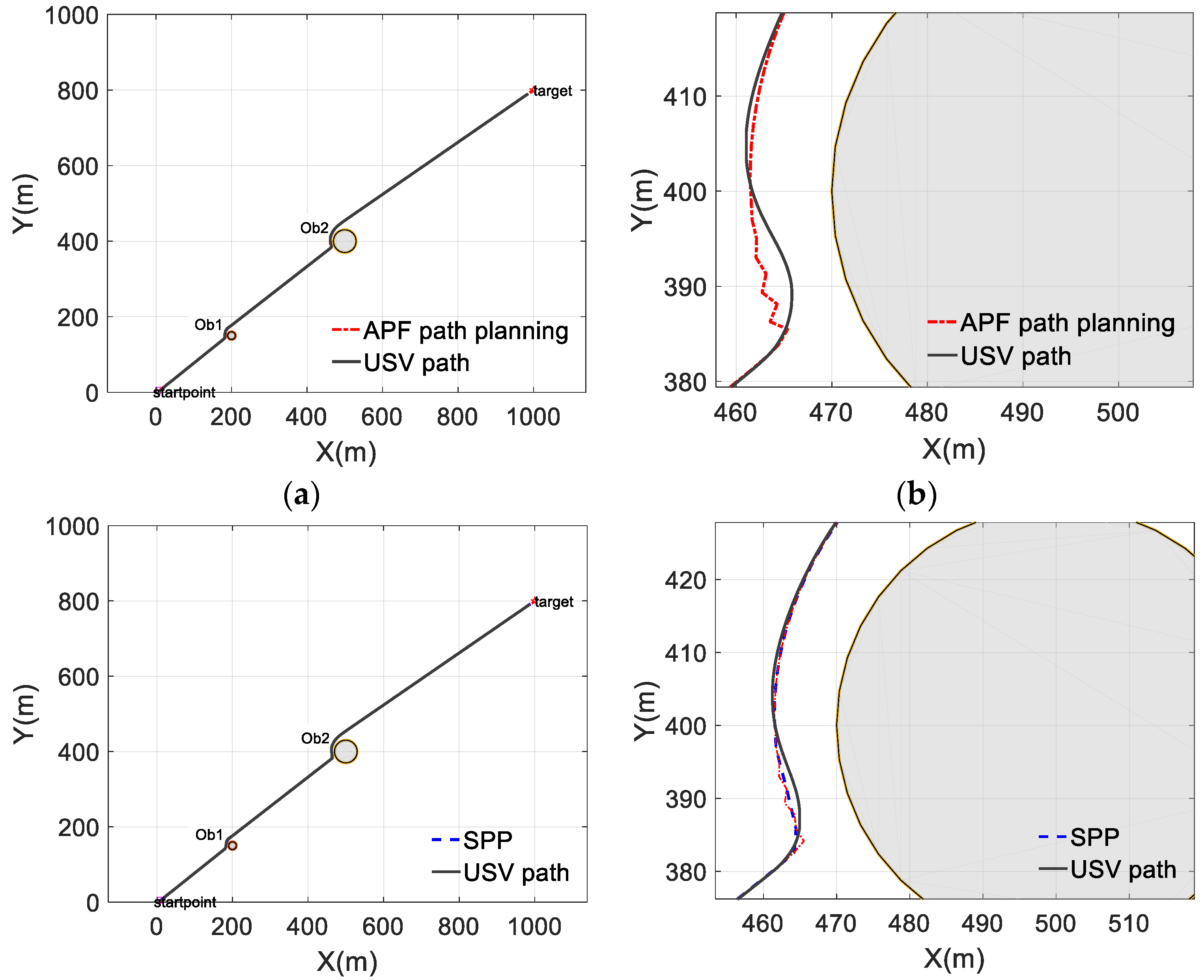
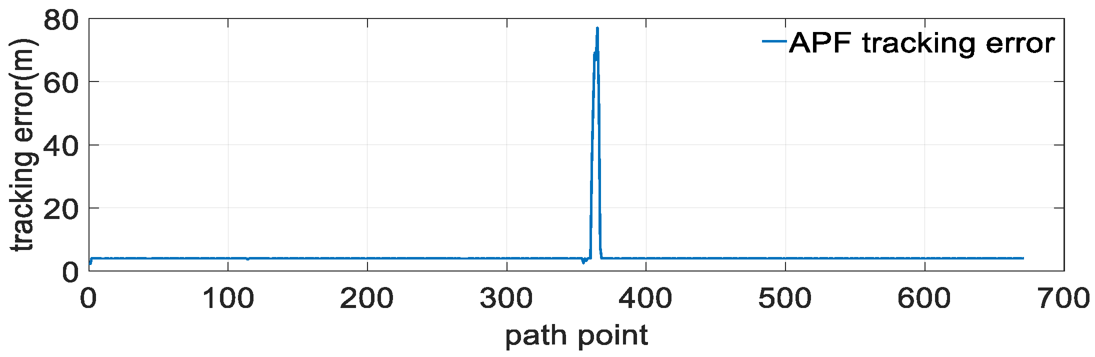
4.2. Comparative Experiment of Large Planning Step

With the same simulation environment and control parameters as in the abovementioned experiment, the USV sailed from the same position to the same target, and the planning step, t p , was set greater than the length of the vehicle by a factor of 5 ( t p = 10.0 m). The results of the comparison between the two methods with respect to the USV trajectory tracking are respectively shown in Figure 16a,b.
As can be seen from Figure 16a, the USV generated roundabout routes when it tracked the planned path points during its approach of the first and second obstacles, which resulted in a failure to complete the obstacle avoidance task (given that the obstacle was a virtual object in the simulation, the task was not interrupted due to collision, and the experiment was continued). Figure 17 presents the tracking deviation of the USV for the duration of the trajectory tracking task. A maximum path deviation of 34 m was generated near the first obstacle, which gradually decreased to a value of approximately 4.0 m, and then remained stable. It should be noted that the distance between the navigation position of the vehicle and the tracking target was reduced to 4.0 m in the simulation; thus, the task was considered as completed. In the vicinity of the second obstacle, the maximum deviation was approximately 77.0 m, and due to its course deviation, the tracking process always sailed in an approximate 3/4 minimum turning circle in the following trajectory tracking process. This resulted in the oscillation of the tracking deviation within the range of 8 m until the target point was reached.
According to the analysis results in Figure 16b and Figure 18, during the large planning step, the USV tracked the planned path optimized by the secondary planning, and then successfully completed the obstacle avoidance task. The tracking deviation, namely, the along track error, was less than 4 m; thus, the vehicle was considered to reach the target point. As can be seen from Figure 18, the obstacle has no effect on the tracking accuracy, and the tracking deviation was approximately 4 m. Figure 17 and Figure 18 illustrate the decrease in the number of track points after optimization, which reduced the possibility of the occurrence of detour road events. The experimental results indicate that the SPP method improves the tracking accuracy of the USV and reduces the length of the detour route, thus reducing the energy consumption and preventing collisions.

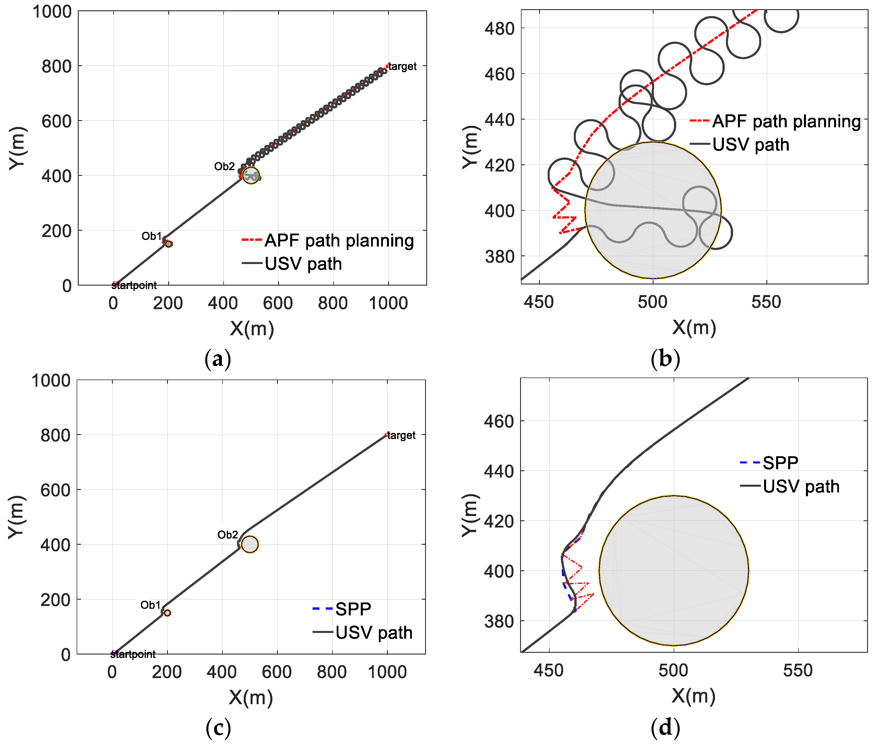
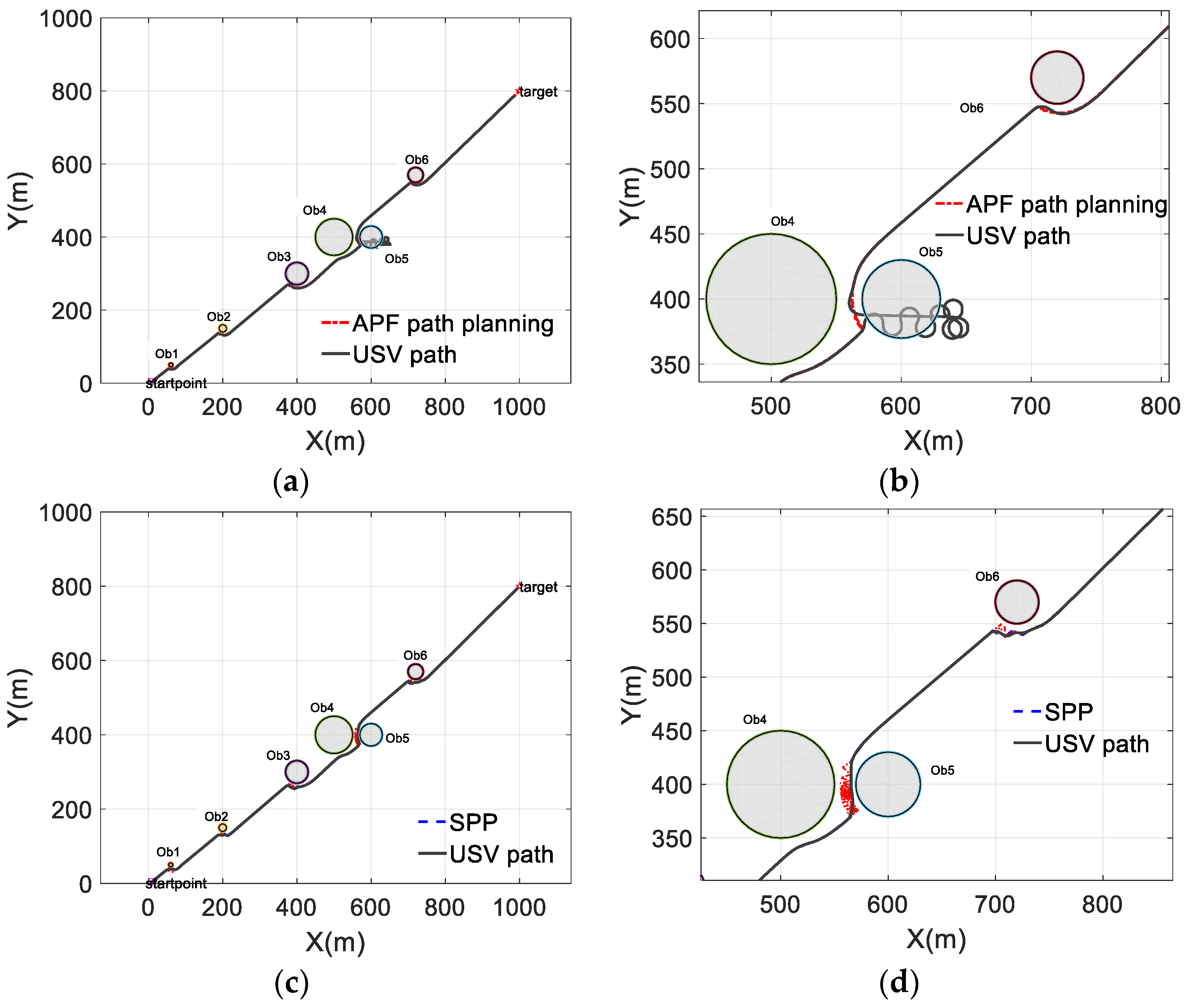
4.3. Comparative Experiment of Multi-Obstacle Path Planning

According to the abovementioned experiment, in the case of two obstacles in the small planning step, the USV successfully tracked the path planned by APF and SPP, and completed the obstacle avoidance task. With an identical simulation environment and control parameters to those of the abovementioned experiment, the vehicle navigated from the same starting position to the same target point, thus avoiding six obstacles in the course, which had position coordinates of (60 m, 50 m), (200 m, 150 m), (400 m, 300 m), (500 m, 400 m), (600 m, 400 m), and (720 m, 570 m). In addition, the obstacle radius corresponded to 5.0 m, 10.0 m, 30.0 m, 50.0 m, 30.0 m, and 20.0 m, respectively. The results of the comparison between the initial path planning utilizing the improved artificial potential field method and the second path planning under the consideration of the motion performance of the USV are shown in Figure 19a,b. The trajectory tracking deviations for the two methods are shown in Figure 20 and Figure 21.
As can be seen from Figure 19a and Figure 20, using the APF method, the USV successfully completed the obstacle avoidance task of the first three obstacles, and the trajectory tracking deviation was constant at approximately 4 m. However, when sailing near the fourth and fifth obstacles, due to the limitation of the motion performance of the vehicle, the planned path exceeded its minimum turning radius, which resulted in a collision with the fifth obstacle. Moreover, the trajectory tracking deviation was approximately 78 m, and the obstacle avoidance task was not completed.
Figure 19b and Figure 21 reveal that on the basis of the SPP method, the USV successfully completed the obstacle avoidance task of all six obstacles, and the track tracking deviation was constant at approximately 4.0 m. The optimized path of the second path planning method can therefore effectively ensure the completion efficiency of the obstacle avoidance task and improve the precision of the trajectory tracking control.

5. Discussion

(1)
By the analysis of the path planning theory and the USV control model, the traditional path planning method was found to lead to the ‘planning failure’ phenomenon when applied to the trajectory tracking field of the USV path planning.
(2)
In this study, an integral nonlinear least squares method was developed. In the case of limited test data, a nonlinear motion model of USV was rapidly identified by merely conducting a type of maneuvering experiment, which can effectively predict the motion performance indexes, such as the rotatory curvature of the vehicle.
(3)
The SPP method was presented under the consideration of the USV motion performance, which reduces the influence of the motion performance of the vehicle during the trajectory tracking and helps lower the risk of failing to complete the obstacle avoidance task using the traditional path planning method. The proposed SPP method can effectively prevent the issue of an untraceable USV and improve the USV tracking accuracy.

6. Conclusions

This paper presented an integral nonlinear least squares method to rapidly and effectively obtain the motion constraint of USVs, and an SPP method was proposed under the consideration of the USV motion performance.
In future work, the path optimization method in a bounded environment, especially an uneven boundary, should be considered. In addition, a field test of the method should be carried out.

Author Contributions

Conceptualization, Y.L. (Ye Li) and J.F.; methodology, Y.L. (Yulei Liao) and J.F.; software, J.F. and W.J.; validation, Y.L. (Ye Li), J.F. and L.W.; formal analysis, H.W.; investigation, W.J. and H.W.; data curation, J.F. and W.J.; writing—Original draft preparation, J.F.; writing—review and editing, J.F. and Q.J.; supervision, Y.L. (Ye Li) and Y.L. (Yulei Liao); funding acquisition, Y.L. (Ye Li) and Y.L. (Yulei Liao) Authorship has been limited to those who have contributed substantially to the work reported.

Funding

This research was funded by the National Key R&D Program of China under Grant 2017YFC0305700, in part by the National Natural Science Foundation of China under Grant 51779052, U1806228, and 51879057, in part by the Natural Science Foundation of Heilongjiang Province of China under Grant QC2016062, in part by the Research Fund from Science and Technology on Underwater Vehicle Laboratory under Grant 614221503091701, in part by the Fundamental Research Funds for the Central Universities under Grant HEUCFP201741, and HEUCFG201810, and in part by the Qingdao National Laboratory for Marine Science and Technology under Grant QNLM2016ORP0406.

Conflicts of Interest

The authors declare no conflict of interest.

References

  1. Liao, Y.L.; Zhang, M.J.; Wan, L.; Li, Y. Trajectory tracking control for underactuated unmanned surface vehicles with dynamic uncertainties. J. Cent. South Univ. Technol. 2016, 23, 370–378. [Google Scholar] [CrossRef]
  2. Li, Y.; Wang, L.F.; Liao, Y.L.; Jiang, Q.Q.; Pan, K.W. Heading MFA control for unmanned surface vehicle with angular velocity guidance. Appl. Ocean Res. 2018, 80, 57–65. [Google Scholar] [CrossRef]
  3. Liu, Y.; Bucknall, R. A survey of formation control and motion planning of multiple unmanned vehicles. Robotica 2018, 36, 1019–1047. [Google Scholar] [CrossRef]
  4. Singh, Y.; Sharma, S.; Sutton, R.; Hatton, D. Path planning of an autonomous surface vehicle based on artificial potential fields in a real-time marine environment. In Proceedings of the 16th International Conference on Computer and IT Applications in the Maritime Industries, Cardiff, UK, 15–17 May 2017. [Google Scholar]
  5. Singh, Y.; Sharma, S.; Sutton, R.; Hatton, D.; Khan, A. Feasibility study of a constrained Dijkstra approach for optimal path planning of an unmanned surface vehicle in a dynamic maritime environment. In Proceedings of the 2018 IEEE International Conference on Autonomous Robot Systems and Competitions (ICARSC), Torres Vedras, Portugal, 25–27 April 2018; pp. 117–122. [Google Scholar]
  6. Fu, B.; Chen, L.; Zhou, Y.T.; Zheng, D. An improved A algorithm for the industrial robot path planning with high success rate and short length. Robot. Auton. Syst. 2018, 106, 26–37. [Google Scholar] [CrossRef]
  7. Singh, Y.; Sharma, S.; Sutton, R.; Hatton, D.; Khan, A. A constrained A* approach towards optimal path planning for an unmanned surface vehicle in a maritime environment containing dynamic obstacles and ocean currents. Ocean Eng. 2018, 169, 187–201. [Google Scholar] [CrossRef]
  8. Zhu, L.; Fan, J.Z.; Zhao, J.; Wu, X.G.; Liu, G. Global path planning and local obstacle avoidance of searching robot in mine disasters based on grid method. J. Cent. South Univ. 2011, 11, 3421–3428. [Google Scholar]
  9. Qu, Y.H.; Zhang, Y.T.; Zhang, Y.M. A global path planning algorithm for fixed-wing UAVs. J. Intell. Robot. Syst. 2018, 91, 691–707. [Google Scholar] [CrossRef]
  10. Sfeir, J.; Saad, M.; Saliah, H. An improved artificial potential field approach to real –time mobile robot path planning in an unknown environment. In Proceedings of the IEEE International Symposium on Robotic and Sensors Environments, Montreal, QC, Canada, 17–18 September 2011; pp. 208–213. [Google Scholar]
  11. Pei, Z.B.; Chen, X.B. Improved ant colony algorithm and its application in obstacle avoidance for robot. CAAI Trans. Intell. Syst. 2015, 1, 90–96. [Google Scholar]
  12. Wang, J.; Wu, X.X.; Guo, B.L. Robot path planning using improved particle swarm optimization. Comput. Eng. Appl. 2012, 48, 240–244. [Google Scholar]
  13. Yan, Z.P.; Li, J.Y.; Wu, Y.; Zhang, G.S. A real-time path planning algorithm for AUV in unknown underwater environment based on combining PSO and waypoint guidance. Sensors 2019, 19, 20. [Google Scholar] [CrossRef] [PubMed]
  14. Wang, H.W.; Ma, Y.; Xie, Y.; Guo, M. Mobile robot optimal path planning based on smoothing A* algorithm. J. Tongji Univ. (Nat. Sci.) 2010, 38, 1647–1650. [Google Scholar]
  15. Conte, G.; Capua, G.P.; Scaradozzi, D. Designing the NGC system of a small ASV for tracking underwater targets. Robot. Auton. Syst. 2016, 76, 46–57. [Google Scholar] [CrossRef]
  16. Doostie, S.; Hoshiar, A.K.; Nazarahari, M. Optimal path planning of multiple nanoparticles in continuous environment using a novel Adaptive Genetic Algorithm. Precis. Eng. 2018, 53, 65–78. [Google Scholar] [CrossRef]
  17. Wu, C.; Wu, Q.; Ma, F.; Wang, S.W. A situation awareness approach for USV based on Artificial Potential Fields. In Proceedings of the International Conference on Transportation Information and Safety 2017, Banff, AB, Canada, 8–10 August 2017; pp. 232–235. [Google Scholar]
  18. Yang, J.M.; Tseng, C.M.; Tseng, P.S. Path planning on satellite images for unmanned surface vehicles. Int. J. Nav. Archit. Ocean Eng. 2015, 7, 87–99. [Google Scholar] [CrossRef]
  19. Abbas, S.; Abbas, K.; Troy, R.; Saeid, N. Smooth path planning using biclothoid fillets for high speed CNC machines. Int. J. Mach. Tools Manuf. 2018, 132, 36–49. [Google Scholar]
  20. Brezak, M.; Petrovic, I. Path smooth using clothoids for differential drive mobile robots. IFAC Proc. Vol. 2011, 44, 1133–1138. [Google Scholar] [CrossRef]
  21. Shi, W.F.; Huang, X.H.; Zhou, W. Planning of mobile robot based on improved artificial potential. J. Comput. Appl. 2010, 30, 2021–2023. [Google Scholar]
  22. Liao, Y.L.; Zhang, M.J.; Wan, L. Serret-Frenet frame based on path following control for underactuated unmanned surface vehicles with dynamic uncertainties. J. Cent. South Univ. Technol. 2015, 22, 214–223. [Google Scholar] [CrossRef]
  23. Nomoto, K.; Taguchi, K.; Honda, K.; Hirano, S. On the steering qualities of ships. Int. Shipbuild. Prog. 1957, 4, 354–370. [Google Scholar] [CrossRef]
  24. Christian, R.S.; Craig, A.W. Modeling, identification, and control of an unmanned surface vehicle. J. Field Robot. 2013, 30, 371–398. [Google Scholar]
  25. Nikola, M.; Zoran, V. Fast in-field identification of unmanned marine vehicles. J. Field Robot. 2011, 28, 101–120. [Google Scholar]
  26. Podisuk, M.; Chundang, U.; Sanprasert, W. Single step formulas and multi-step formulas of the integration method for solving the initial value problem of ordinary differential equation. Appl. Math. Comput. 2007, 190, 1438–1444. [Google Scholar] [CrossRef]
  27. Li, H.L.; Zhang, A.W.; Meng, X.G.; Hu, S.X. A remote sensing image sub-pixel registration method based on curve fitting and improved Fourier-Mellin transform. J. Chin. Comput. Syst. 2015, 36, 2763–2768. [Google Scholar]
  28. Liao, Y.L.; Li, Y.M.; Wang, L.F.; Li, Y.; Jiang, Q.Q. The heading control method and experiments for an unmanned wave glider. J. Cent. South Univ. Technol. 2017, 24, 1–9. [Google Scholar] [CrossRef]
  29. Pradhan, S.K.; Parhi, D.H.; Panda, A.K. Potential field method to navigate several mobile robots. Appl. Intell. 2006, 25, 321–333. [Google Scholar] [CrossRef]
  30. Liu, Z.X.; Yang, L.X.; Wang, J.G. Soccer robot path planning based on evolutionary artificial field. Adv. Mater. Res. 2012, 562, 955–958. [Google Scholar] [CrossRef]
  31. Koren, Y.; Borenstein, J. Potential field methods and their inherent limitations for mobile robot navigation. In Proceedings of the IEEE International Conference on Robotics and Automation, Sacramento, CA, USA, 9–11 April 1991; Volume 2, pp. 1398–1404. [Google Scholar]
  32. Liang, K.; Li, Z.Y.; Chen, D.Y. Improved artificial potential field for unknown narrow environments. In Proceedings of the IEEE International Conference on ROBIO, Shenyang, China, 22–26 August 2004; pp. 688–692. [Google Scholar]
  33. Geva, Y.; Shapiro, A. A combined potential function and graph search approach for free gait generation of quadruped robots. In Proceedings of the IEEE International Conference on Robotics and Automation River Centre, Saint Paul, MN, USA, 14–18 May 2012; pp. 5371–5376. [Google Scholar]
  34. Qi, N.N.; Ma, B.J.; Liu, X.E.; Zhang, Z.X.; Ren, D.C. A modified Artificial Potential Field Algorithm for Mobile Robot Path Planning. In Proceedings of the 7th World Congress on Intelligent Control and Automation, Chongqing, China, 25–27 June 2008; Volume 7, pp. 2603–2607. [Google Scholar]
  35. Liao, Y.L.; Wang, L.F.; Li, Y.M.; Li, Y.; Jiang, Q.Q. The intelligent control system and experiments for an unmanned wave glider. PLoS ONE 2016, 11, 1–24. [Google Scholar] [CrossRef]
  36. Liao, Y.L.; Jia, Z.H.; Zhang, W.B.; Jia, Q.; Li, Y. Layered berthing method and experiment of unmanned surface vehicle based on multiple constraints analysis. Appl. Ocean Res. 2019, 86, 47–60. [Google Scholar] [CrossRef]
  37. Liao, Y.L.; Jiang, Q.Q.; Du, T.P.; Jiang, W. Redefined output model-free adaptive control method and unmanned surface vehicle heading control. IEEE J. Ocean. Eng. 2019. [Google Scholar] [CrossRef]
Figure 1. USV coordinate system.
Jmse 07 00104 g001
Figure 2. The ‘Dolphin 1’ developed by Harbin Engineering University.
Jmse 07 00104 g002
Figure 3. The zig zag test.
Jmse 07 00104 g003
Figure 4. K and T from the zig zag test.
Jmse 07 00104 g004
Figure 5. (a) Description of heading angle fitting curve; (b) the distribution of heading angular velocity; (c) the first part of the heading angular velocity’s fitting curve; and (d) the second part of the heading angular velocity’s fitting curve.
Jmse 07 00104 g005
Figure 6. Comparison between the actual and predicted Z-type manipulation.
Jmse 07 00104 g006
Figure 7. Description of the Z-type error curve.
Jmse 07 00104 g007
Figure 8. Comparison between the actual and predicted speed.
Jmse 07 00104 g008
Figure 9. Description of the speed error curve.
Jmse 07 00104 g009
Figure 10. Description of the turning circle simulation test.
Jmse 07 00104 g010
Figure 11. Description of ‘Dolphin 1’ field turning test.
Jmse 07 00104 g011
Figure 12. The schematic diagram of the second path planning.
Jmse 07 00104 g012
Figure 13. The theoretical block diagram of SPP.
Jmse 07 00104 g013
Figure 14. (a) Description of the path planning comparison diagram; and (b) local enlargement of the first obstacle area for path planning.
Jmse 07 00104 g014
Figure 15. (a) Description of USV trajectory by APF; (b) local enlargement of the second obstacle area for the USV trajectory by APF; (c) description of the USV trajectory by SPP; and (d) local enlargement of the second obstacle area for the USV trajectory by SPP.
Jmse 07 00104 g015
Figure 16. (a) Description of the USV trajectory by APF; (b) local enlargement of the second obstacle area for the USV trajectory by APF; (c) description of the USV trajectory by SPP; and (d) local enlargement of the second obstacle area for the USV trajectory by SPP.
Jmse 07 00104 g016
Figure 17. Description of the USV along tracking error by APF.
Jmse 07 00104 g017
Figure 18. Description of the USV along tracking error by SPP.
Jmse 07 00104 g018
Figure 19. (a) Description of the USV trajectory by APF; (b) local enlargement for the USV trajectory by APF; (c) description of the USV trajectory by SPP; and (d) local enlargement for the USV trajectory by SPP.
Jmse 07 00104 g019
Figure 20. Description of the USV along tracking error by APF.
Jmse 07 00104 g020
Figure 21. Description of the USV along tracking error by SPP.
Jmse 07 00104 g021
Table 1. Coefficient.
n C k ( n )
1 1 2 1 2 ///
2 1 6 4 6 1 6 //
3 1 8 3 8 3 8 1 8 /
4 7 90 32 90 12 90 32 90 7 90

