Article

UUV Simulation Modeling and its Control Method: Simulation and Experimental Studies

Marine Robotics R&D Division, Korea Institute of Robot and Convergence, Jigok-Ro 39, Nam-Gu, Pohang 37666, Korea
*
Author to whom correspondence should be addressed.
J. Mar. Sci. Eng. 2019, 7(4), 89; https://doi.org/10.3390/jmse7040089
Submission received: 27 February 2019 / Revised: 24 March 2019 / Accepted: 25 March 2019 / Published: 28 March 2019
(This article belongs to the Special Issue Intelligent Marine Robotics Modelling, Simulation and Applications)

Abstract

:
This paper presents the development of an unmanned underwater vehicle (UUV) platform, especially the derivation of the vehicle’s simulation model and its control method to overcome strong sea current. The platform is designed to have a flattened ellipsoidal exterior so as to minimize the hydrodynamic damping on the horizontal plane. Four horizontal thrusters with the identical specifications are symmetrically mounted on the horizontal plane, and each of them has the same thrust dynamics in both forward and reverse directions. In addition, there are three vertical thrusters used to handle the vehicle’s roll, pitch and heave motions. Control strategy proposed in this paper to overcome strong current is that: maximizing the vectored horizontal thrust force against the sea current without or with the least of the vehicle’s rotation on the horizontal plane. For the vehicle model, due to it being symmetric in all of three axes, the vehicle dynamics can be simplified and all of hydrodynamic coefficients are calculated through both of theoretical and empirically-derived formulas. Numerical simulations and experimental studies in both of the water tank and the circulating water channel are carried out to demonstrate the vehicle’s capability of overcoming strong current.

1. Introduction

In the sea around the Korean peninsula, especially in the West Sea also known as the Yellow Sea, strong sea currents usually pose tough technical challenges in the salvage operations as well as in the various scientific activities. In both cases of ROKS Cheonan sinking on 26 March 2010 [1] and sinking of MV Sewol on 16 April 2014 [2], one of the most difficult problems during the initial response for salvage was that there was not any underwater vehicle able to be deployed in the strong sea current environment [3] so as to collect the swift on-site disaster scene information. Recently, how to overcome strong sea current has become a hot topic in the UUV community, especially in Korea. In [4], a ROV called Crabster CR200 was introduced. The vehicle has about 188 kg of negative buoyancy in the water. So in the case of strong current which can be up to 3 knots, the vehicle can land on the sea floor and using its 6 legs can resist the current. In [5], the authors presented a two-body vehicle, where the lower body can land on the sea floor and overcome strong current using a sort of anchor system. In both cases, the whole vehicle or part of the body should be land on the sea floor to resist the sea current. This kind of mechanism might constrain the vehicle’s precise underwater inspection capability. Other attempts to counter strong turbulence using the high velocity water itself include [6].
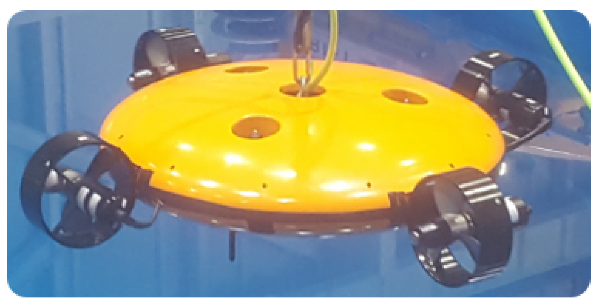
This paper presents the development of a UUV platform and its motion control technology for the purpose of overcoming strong sea current. The vehicle has the flattened ellipsoidal exterior to minimize the hydrodynamic damping in the water, as seen in 
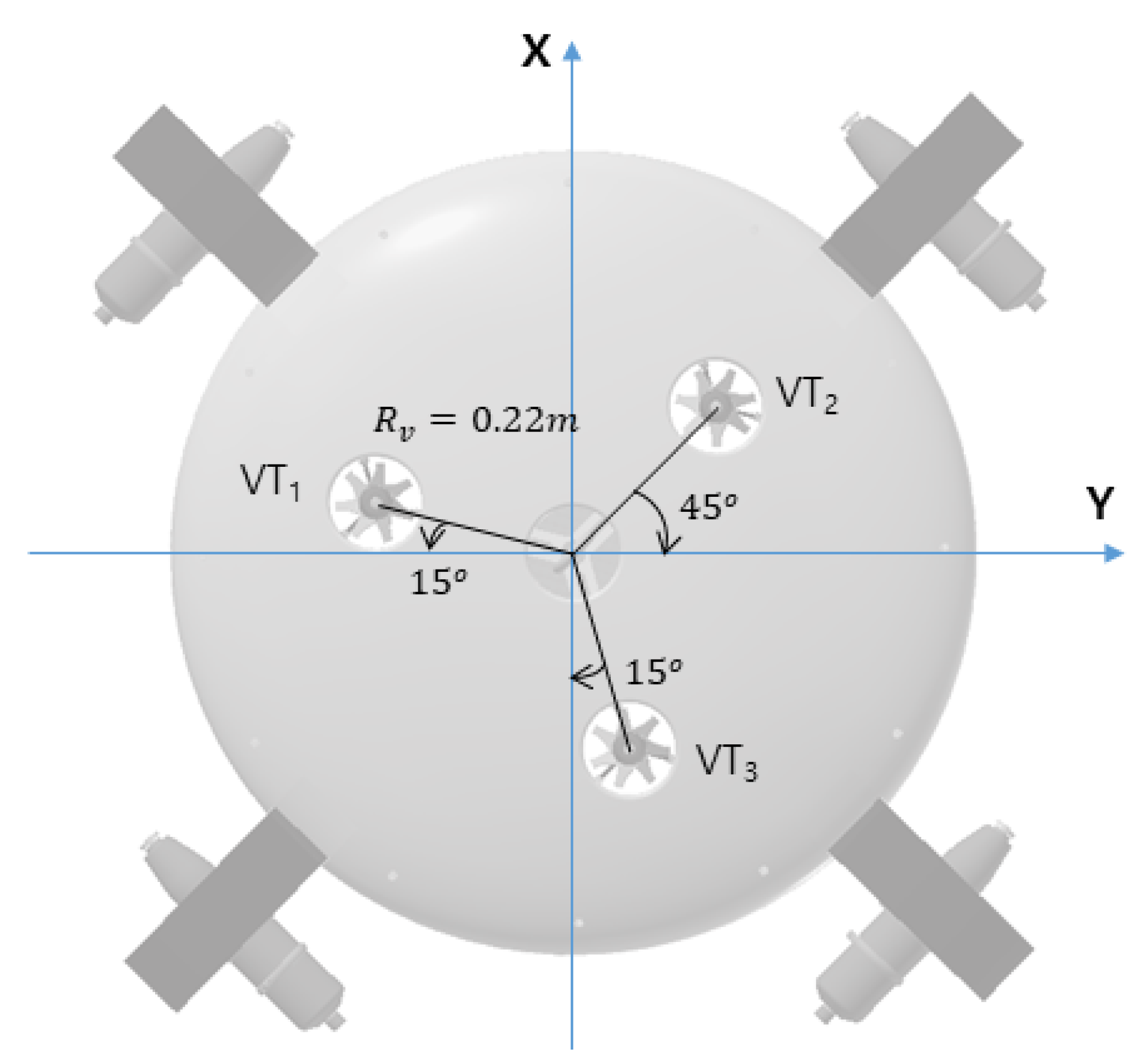
Figure 1. Four horizontal thrusters with the identical specification are mounted symmetrically on the horizontal plane. Each thruster has the same thrust dynamics in both forward and reverse directions. This kind of horizontal thrust mechanism can guarantee the uniform distribution of vectored thrust forces in all horizontal directions. On the other hand, this is also beneficial for easily stabilizing the vehicle’s horizontal motion in the dynamic sea current environment. Three vertical thrusters, as seen in Figure 1, are used to stabilize the vehicle’s roll, pitch, and heave motions.
The control strategy for this vehicle to overcome strong current is to maximize the vectored horizontal thrust force along certain direction, usually against the sea current, while keeping its heading or with the least of heading rotation on the horizontal plane. Three vertical thrusters, as mentioned before, are used to stabilize the roll, pitch and heave motion. General PD controllers [7,8] are designed independently for each of the horizontal and vertical thrusters groups.
Some of the simulation and experimental studies are carried out to demonstrate the performance of the platform design and its motion control technologies. In the simulation, the hydrodynamic coefficients are calculated through both of the theoretical and empirically-derived formulas [9,10,11]. Furthermore, in the controller design, four horizontal thrusters are modeled under the consideration of the fact that the maximum thrust force will be reduced in compliance with the increasing of fluid speed flow through the thruster [12,13]. In addition, through circulating water channel test, it is observed that the vehicle can get forward motion while keeping its heading in the strong current environment where the current is up to 2.5 knots.
The remainder of this paper is organized as follows. 
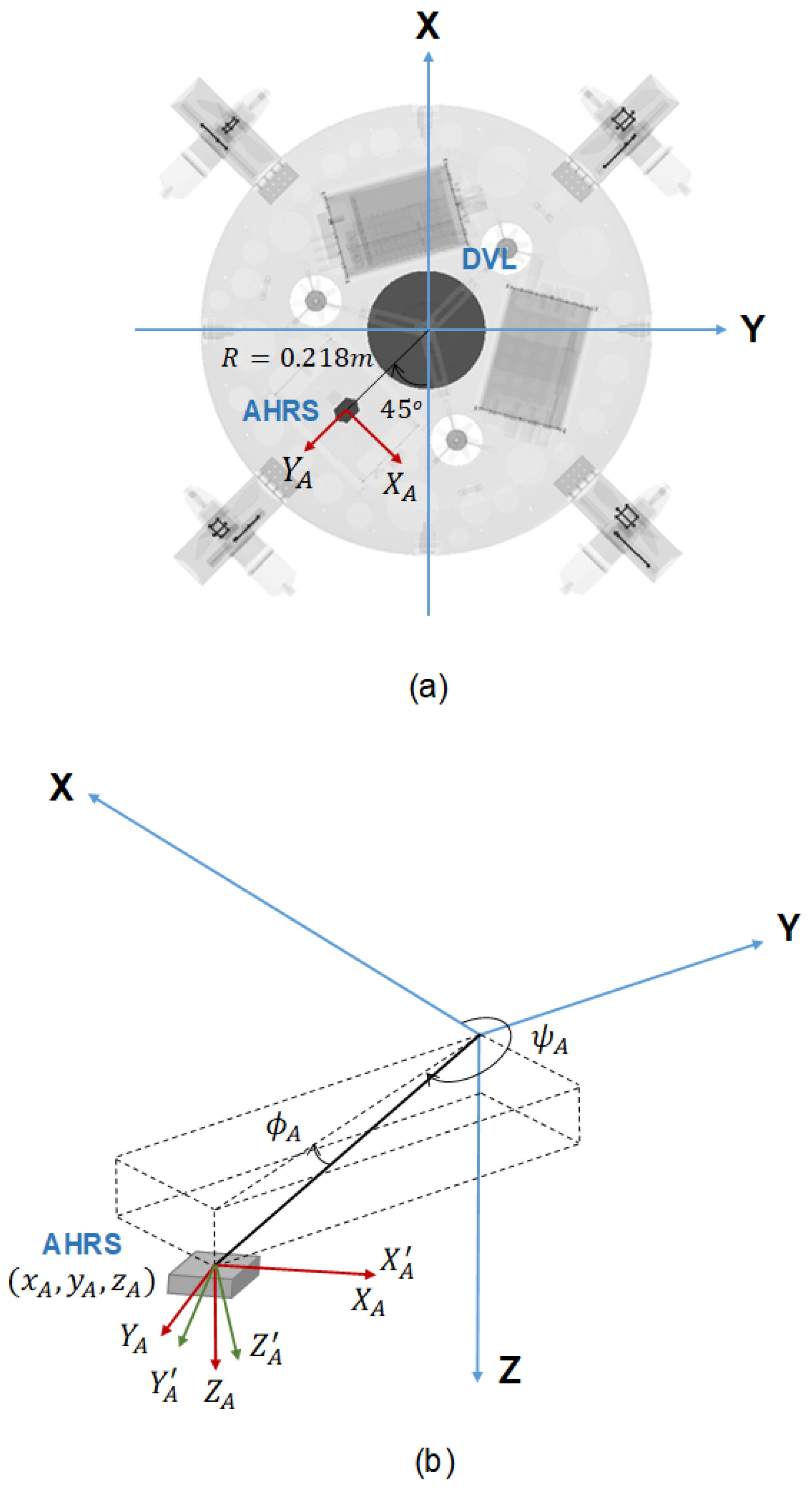
Section 2 describes the vehicle’s kinematic and hydrodynamic model, and the vehicle motion sensor’s lever arm effects are considered in Section 3. Controllers for both of horizon keeping and maximum forward speed on the horizontal plane are presented in Section 4. Furthermore, Section 5 shows the simulation result, while experimental studies are presented in Section 6. A brief conclusion and some future works are discussed in Section 7.

2. Vehicle Modeling

2.1. Kinematics and Dynamics

Usually, the kinematics and dynamics of underwater vehicles can be expressed as follows [9],
η ˙ = C b n ν ,
M R B ν ˙ + C R B ν = F e x t ,
where η = [ x , y , z , ϕ , θ , ψ ] T is the position and attitude vector defined in the navigation frame (NED-frame), and ν = [ u , v , w , p , q , r ] T is the linear and angular velocity vector defined in the vehicle’s body-fixed frame; and C b n denotes the coordinate transformation matrix from the body-fixed frame to the navigation frame, and can be expressed as
C b n = J 1 0 3 × 3 0 3 × 3 J 2
where
J 1 = c ψ c θ s ψ c ϕ + c ψ s θ s ϕ s ψ s ϕ + c ψ s θ c ϕ s ψ c θ c ψ c ϕ + s ψ s θ s ϕ c ψ s ϕ + s ψ s θ c ϕ s θ c θ s ϕ c θ c ϕ , J 2 = 1 s ϕ t θ c ϕ t θ 0 c ϕ s ϕ 0 s ϕ / c θ c ϕ / c θ ,
with s ( · ) = s i n ( · ) , c ( · ) = c o s ( · ) , t ( · ) = t a n ( · ) .
For the vehicle developed as seen in Figure 1, its body-fixed frame is centered at the vehicle’s buoyancy center as in [11] and the weight center is located at ( x g , y g , z g ) = ( 0 , 0 , 4 . 51 mm ) after being neutrally ballasted. Therefore, the rigid-body inertia matrix M R B and Coriolis and centripetal matrix C R B can be simplified as follows
M R B = m 0 0 0 m z g 0 0 m 0 m z g 0 0 0 0 m 0 0 0 0 m z g 0 I x x 0 0 m z g 0 0 0 I y y 0 0 0 0 0 0 I z z ,
C R B = 0 0 0 m z g r m w m v 0 0 0 m w m z g r m u 0 0 0 m ( z g p v ) m ( z g q + u ) 0 m z g r m w m ( z g p v ) 0 I z z r I y y q 0 m z g r m z g q I z z r 0 I x x p 0 0 0 I y y q I x x p 0 ,
where m = 58.94 kg is the rigid body mass, and I x x , I y y , and I z z denote the inertia moments each along the X , Y , and Z axes. Calculated inertia moments are as shown in Table 1.
For the vehicle dynamics as in (2), the sum of external forces and moments can be expressed as follows as in [9,11]
F e x t = F h y d r o s t a t i c s + F d r a g + F a d d e d _ m a s s + F c o n t r o l ,
where F h y d r o s t a t i c s = [ 0 , 0 , 0 , z g W c θ s ϕ , z g W s θ , 0 ] T with W the rigid body weight.

2.2. Hydrodynamic Damping Term F d r a g

The vehicle is symmetric along all three of X , Y , and Z axes, see Figure 1. Therefore, the movement-induced moments A b | b | with A = { K , M , N } and b = { u , v , w } , and the rotation-induced forces B a | a | with B = { X , Y , Z } and a = { p , q , r } are all negligible. In addition, to simplify the vehicle’s model and therefore to avoid complicated mathematical calculations, the following assumptions similar to [11] are made in the vehicle modeling, where [14] describes deterministic artificial intelligence methods to deal with coupled disturbances. Preliminary research in overcome linear coupling is contained in [15], while methods to counter angular coupling is described in [16], following an established lineage of continuing research from [17,18,19,20,21,22,23].
  • Linear and angular coupled damping terms are ignorable.
  • Any damping terms greater than second-order are negligible.
Consequently, F d r a g can be simplified as
F d r a g = [ X u | u | u | u | , Y v | v | v | v | , Z w | w | w | w | , K p | p | p | p | , M q | q | q | q | , N r | r | r | r | ] T .
Corresponding coefficients are calculated using the following formulas
X u | u | = Y v | v | = 0.5 ρ c d c π a R 4 ( 0.5 ρ s D c d D ) ,
Z w | w | = 0.5 ρ c d c π R 2 4 ( 0.5 ρ s F c d F ) ,
K p | p | = M q | q | = 2 0.5 ρ c d c 0 R D ( r ) r 3 d r 2 x T F 3 ( 0.5 ρ s F c d F ) ,
N r | r | = 2 0.5 ρ c d c 0 R D ( r ) r 3 d r 2 x T D 3 ( 0.5 ρ s D c d D ) ,
where a = 0.128 m , R = 0.435 m , x T F = x T D = 0.543 m , s F = 0.163 m 2 , s D = 0.023 m 2 , and the drag coefficients are derived through empirical graph as Figure 2.4 in (p. 19, [1]), and selected as c d c = 1.12 , c d c = 0.3 , c d F = 0.63 , c d D = 0.9 .
Calculated coefficients are shown in Table 2.

2.3. Added Mass Term F a d d e d _ m a s s

As mentioned before, the vehicle is symmetric in all three axes. Therefore, only the diagonal terms in the vehicle’s added mass matrix are considered in this paper. The coefficients are estimated through empirical graph as Figure 4.8 in Newman [10] (p. 147), and calculated as shown in Table 3.

3. Compensation of Motion Sensors Lever Arm Effect

For the majority of underwater vehicles, the motion sensors such as Doppler Velocity Log (DVL) and Attitude and Heading Reference System (AHRD) cannot be arranged on the same center point or center line. Instead, they are usually separated from each other and also from the center point of the body-fixed frame. Therefore, raw measurements of these motion sensors should be suitably compensated in order to acquire the accurate vehicle motion information, which is further used for the vehicle’s navigation and motion control [24,25].
For the vehicle seen in Figure 1, DVL and AHRS arrangements are as shown in Figure 2a, where DVL is mounted at the center of the body-fixed frame and AHRS is 0.218 m away from the center line.

3.1. Angular Rate Correction

As seen in Figure 2, AHRS body frame X A Y A Z A is rotated from the vehicle’s body-fixed frame X Y Z at ϕ A = 0 , θ A = 0 , ψ A = 135 . For this reason, the angular rate ω = [ p , q , r ] T in the X Y Z frame can be calculated through the following coordinate transformation
p q r = c o s ψ A s i n ψ A 0 s i n ψ A c o s ψ A 0 0 0 1 p r q r r r ,
where ω r = [ p r , q r , r r ] T is the angular velocity measured by AHRS.
Remark 1.
X A Y A Z A and X Y Z are two of fixed frames in the vehicle’s rigid body. In this case, it is necessary to mention that the coordinates transformations of all vectors including angular rate should obey the linear velocity transformation Equation (2.16) in [9], not the angular velocity transformation of Equation (2.26) in [9].

3.2. Acceleration Correction

In the vehicle’s body-fixed frame X Y Z , AHRS center point coordinate is ( x A , y A , z A ) . In addition, lever arm effect usually causes additional acceleration at the AHRS center point in the case of vehicle’s rotation. The velocity V A at the AHRS center point in the frame X A Y A Z A (see Figure 2b) and the velocity V B in the vehicle’s body-fixed frame X Y Z has the following relationship [24,26]
V A = V B + ω × R ,
where R = [ x A , y A , z A ] T .
Differentiating (13), have
V ˙ A = V ˙ B + ω ˙ × R + ω × V B + ω × ( ω × R ) .
From Figure 2b, it is easy to see that the frame X A Y A Z A is tilted from AHRS body frame X A Y A Z A at ϕ A = a t a n ( z A / x A 2 + y A 2 ) . So, it has
V ˙ A = 1 0 0 0 c o s ϕ A s i n ϕ A 0 s i n ϕ A c o s ϕ A V ˙ A H R S = C A H R S A V ˙ A H R S ,
where V ˙ A H R S is the acceleration measurement by AHRS.
Consequently, the acceleration vector V B in the vehicle’s body-fixed frame can be estimated from AHRS measurement through the following equation
V ˙ B = C A H R S A V ˙ A H R S ω ˙ × R ω × V B ω × ( ω × R ) ,
where ω ˙ is the angular acceleration and should be properly calculated. One option is that it can be estimated through a sort of low-pass filter as follows
ω ˙ ( k + 1 ) = ( 1 λ ) ω ˙ ( k ) + λ ω ˙ m ( k + 1 ) , ω ˙ ( 0 ) = ω ˙ m ( 0 ) ,
where ω ˙ m ( k + 1 ) = [ ω ( k + 1 ) ω ( k ) ] / Δ T with Δ T sampling time, and 0 < λ 1 is a design parameter.
Remark 2.
Vehicle’s angular rate ω and acceleration V ˙ B in the body-fixed frame can be calculated through each of (12) and (16). Furthermore, the vehicle’s attitude is calculated by ( ϕ , θ , ψ ) = ( ϕ m , θ m , ψ m ψ A ) , where ( ϕ m , θ m , ψ m ) is the measurement of AHRS and ψ m ψ A is defined in the domain [ 0 , 2 π ) . Since the DVL is located at the center point, its measurement is directly used as V B .

4. Control Design

As mentioned before, the control strategy proposed in this paper to overcome strong current is to maximize the vectored horizontal thrust force along the direction against the current, while keeping the vehicle’s heading or with the minimum heading rotation. To do so, it needs to spread the vectored horizontal thrust force on the horizontal plane as uniformly as possible.

4.1. Maximum Horizontal Vectored Thrust Force
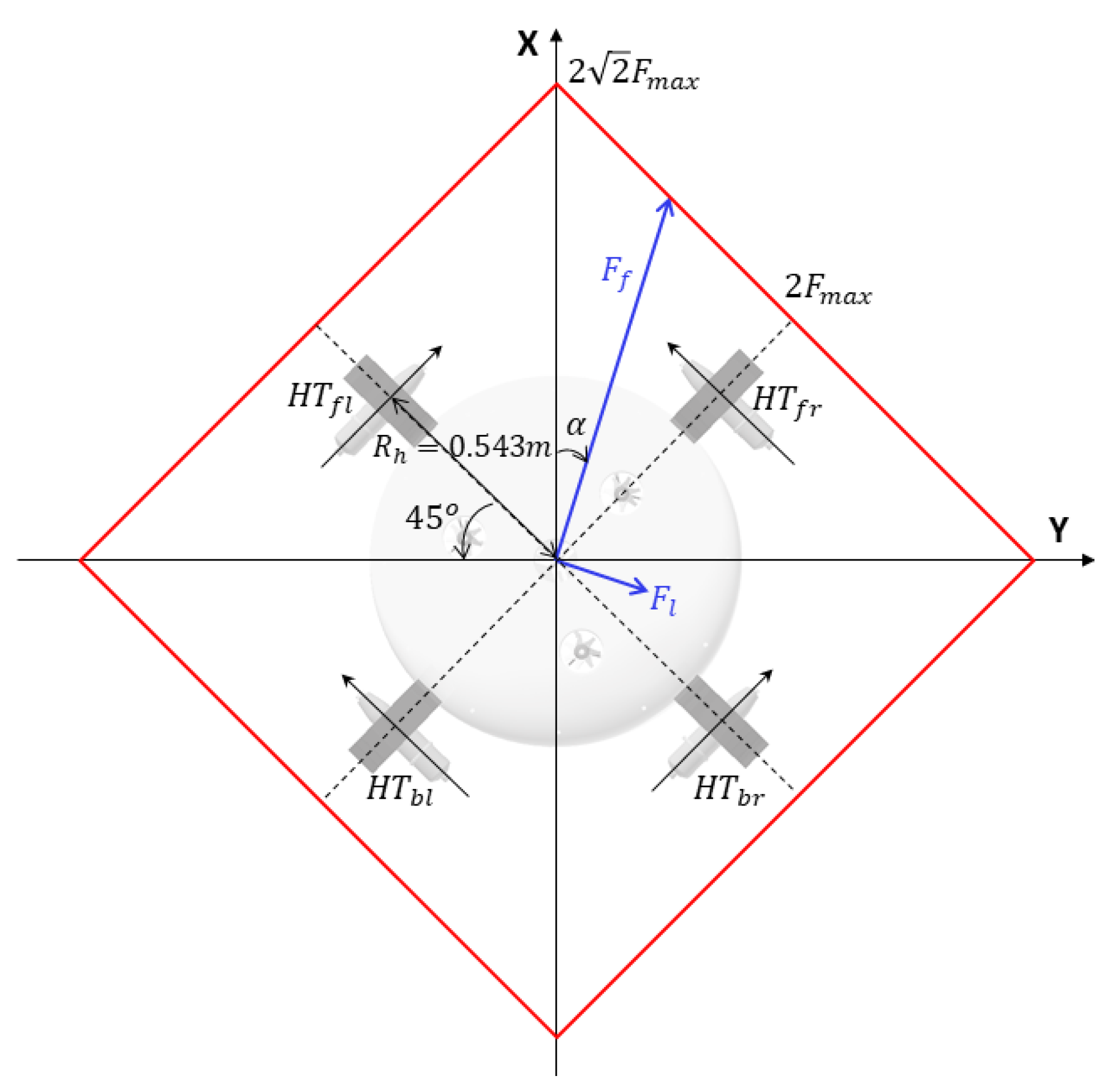
As shown in Figure 3, four horizontal thrusters are mounted symmetrically around the ellipsoidal shape of platform. Each of the thrusters has the same forward and reverse thrust dynamics.
Definition 1.
Given the direction α as seen in Figure 3, the maximum horizontal vectored thrust force means the maximum of F f caused by four symmetrically mounted horizontal thrusters with the following properties
P1.
The orthogonal component F l = 0 .
P2.
Horizontal rotation moment is zero.
Remark 3.
In the case of maximum horizontal vectored thrust force, it has F H T f l = F H T b r and F H T f r = F H T b l where F H T a denotes the thrust force for thruster H T a with a { f l , f r , b r , b l } . For example, consider the case α = 45 . To maximize F f , the thrusters H T f l and H T b r have to take the maximum of forward thrusts. Due to the fact that these four thrusters have the same thrust dynamics, it has F H T f l = F H T b r = F m a x with F m a x the maximum thrust force provided by one thruster. On the other hand, in order to satisfy the P1 and P2 in Definition 1, the remainder thrusters have to set as F H T f r = F H T b l = 0 .
Lemma 1.
Given four of the symmetrically mounted horizontal thrusters as shown in Figure 3, the maximum horizontal vectored thrust force can be calculated as follows
F f = 2 F m a x c o s ( α 45 ) , i f 0 α < 90 2 F m a x c o s ( α + 45 ) , i f 90 α < 180 2 F m a x c o s ( α 45 ) , i f 180 α < 270 2 F m a x c o s ( α + 45 ) , i f 270 α < 360
Proof of Lemma 1.
From Figure 3, it is easy to get
F f = F A c o s ( α 45 ) + F B c o s ( α + 45 ) ,
F l = F A s i n ( α 45 ) + F B s i n ( α + 45 ) ,
where F A = F H T f l + F H T b r and F B = F H T f r + F H T b l .
In order for F l = 0 with (20), it has
F A F B = c o t ( α 45 ) .
Therefore, F A and F B cannot be taken the maximum value at the same time if | c o t ( α 45 ) | 1 . In the case of α { [ 0 , 90 ) [ 180 , 270 ) } , it has | c o t ( α 45 ) | 1 . Substituting F B = F A · t g ( α 45 ) into (19), it can be get
F f = F A c o s ( α 45 ) c o s ( α + 45 ) s i n ( α 45 ) c o s ( α 45 ) = F A c o s ( α 45 ) .
In the case α [ 0 , 90 ) , it has F A = 2 F m a x and if α [ 180 , 270 ) then F A = 2 F m a x . Therefore, (22) can be rewritten as
F f = 2 F m a x c o s ( α 45 ) i f 0 α < 90 , 2 F m a x c o s ( α 45 ) i f 180 α < 270
Similarly, in the case of α { [ 90 , 180 ) [ 270 , 360 ) } , substituting F A = F B c o t ( α 45 ) into (19), have
F f = F B c o s ( α + 45 ) c o s 2 ( α 45 ) s i n ( α 45 ) = F B s i n ( α 45 ) .
If α [ 90 , 180 ) , then F B = 2 F m a x , and if α [ 270 , 360 ) , then F B = 2 F m a x . Consequently, (24) can be rewritten as
F f = 2 F m a x s i n ( α 45 ) i f 90 α < 180 , 2 F m a x s i n ( α 45 ) i f 270 α < 360
Combining (23) and (25) can conclude the Proof.
Remark 4.
Calculated maximum horizontal vectored thrust force field is the red-colored square shown in Figure 3. The maximum vectored thrust force is 2 2 F m a x and minimum value is 2 F m a x . It is easy to see that to align the maximum vectored thrust force with the opposite direction of arbitrarily given sea current, the vehicle’s maximum rotation angle is less than 45 .

4.2. Maximum Forward Speed Controller with Heading-Keeping

One of the important target specifications of this project is the vehicle’s maximum forward speed while keeping its heading angle. Proposed control law is as follows:
i f δ ψ { [ 0 , 45 ) [ 315 , 360 ) }
F H T f l = F H T f r = F m a x
i f d t 0
   F H T b r = F m a x d t ; F H T b l = F m a x
e l s e
   F H T b r = F m a x ; F H T b l = F m a x + d t
e n d
e l s e i f δ ψ [ 45 , 135 )
F H T f r = F m a x ; F H T b r = F m a x
i f d t 0
   F H T b l = F m a x + d t ; F H T f l = F m a x
e l s e
   F H T b l = F m a x ; F H T f l = F m a x + d t
e n d
e l s e i f δ ψ [ 135 , 225 )
F H T b r = F H T b l = F m a x
i f d t 0
   F H T f l = F m a x + d t ; F H T f r = F m a x
e l s e
   F H T f l = F m a x ; F H T f r = F m a x d t
e n d
e l s e
F H T b l = F m a x ; F H T f l = F m a x
i f d t 0
   F H T f r = F m a x d t ; F H T b r = F m a x
e l s e
   F H T f r = F m a x ; F H T b r = F m a x d t
e n d
e n d
where δ ψ = ψ r ψ with ψ r the reference heading and d t = K h p δ ψ + K h d r with K h p and K h d control gain parameters.

4.3. Horizon Keeping Controller

Three vertical thrusters are mounted as seen in Figure 4.

4.3.1. Roll Motion Control

The roll motion control component for V T 1 is designed as
V T r 1 = K v p ( ϕ r ϕ ) + K v d p ,
where ϕ r is the reference roll angle, K v p and K v d are two gain parameters.
In the case of roll motion control, the remainder of two control components V T r 2 and V T r 3 are designed through simultaneously satisfying the following two conditions
C1.
V T r 1 · c o s 15 = V T r 2 · c o s 45 V T r 3 · s i n 15 .
C2.
V T r 1 · s i n 15 + V T r 2 · c o s 45 = V T r 3 · c o s 15 .
Remark 5.
Here, C1 is the condition to balance the right and left torques about the X-axis, and C2 is to neutralize the pitch torque during the roll motion control.
Combining C1 and C2, it is easy to get
V T r 2 = 1.1547 · V T r 1 ,
V T r 3 = 0.5774 · V T r 1 .

4.3.2. Pitch Motion Control

The design procedure is similar to the roll motion control. First, the pitch motion control component for V T 3 is chosen as
V T p 3 = K v p ( θ r θ ) + K v d q ,
where θ r is the reference pitch angle.
Control law for other two vertical thrusters is to simultaneously satisfying the following two conditions
C3.
V T p 3 · c o s 15 = V T p 2 · c o s 45 + V T p 1 · s i n 15 .
C4.
V T p 1 · c o s 15 = V T p 2 · c o s 45 + V T p 3 · s i n 15 .
Remark 6.
Here C3 is to balance the pitch torque about the Y-axis, and C4 is to neutralize the roll torque during the pitch motion control.
Consequently, have
V T p 1 = 0.5774 · V T p 3 ,
V T p 2 = 1.1547 · V T p 3 .
Remark 7.
In both of roll and pitch motion controls, any of three vertical thrusters can be selected and designed its thrust force using (26) or (29), and other two thrusters are designed through simultaneously satisfying C1 and C2, or C3 and C4. In the case of horizon keeping, ϕ r and θ r can be simply set as zero values.

4.3.3. Depth Control

The following simple PD controller is designed for depth control
V T d i = K v p d ( z r z ) + K v d d w , i = 1 , 2 , 3 ,
where V T d i is the depth control component for the thruster V T i , z r is the reference depth, and K v p d and K v d d are gain parameters.

4.4. Thruster Models

4.4.1. Vertical Thruster Model

For each vertical thruster, its thrust versus input relationship is as follows [27]
F V T ( x ) = 74 . 5 N · s a t ( x / 5 ) , i f x 0 31 . 4 N · s a t ( x / 5 ) , i f x < 0
where s a t ( · ) is the saturation function.
Consequently, the thrust force provided by each vertical thruster can be calculated as
F V T i = F V T ( V T r i + V T p i + V T d i ) , i = 1 , 2 , 3 .
Remark 8.
In most of the practical cases, the vehicle takes low speed motion in the vertical direction. For this reason, in the case of vertical thrusters, it is not considered the effect where the thruster’s maximum thrust force decreases in compliance with the increase of the fluid speed flow through the thruster [12].

4.4.2. Horizontal Thruster Model

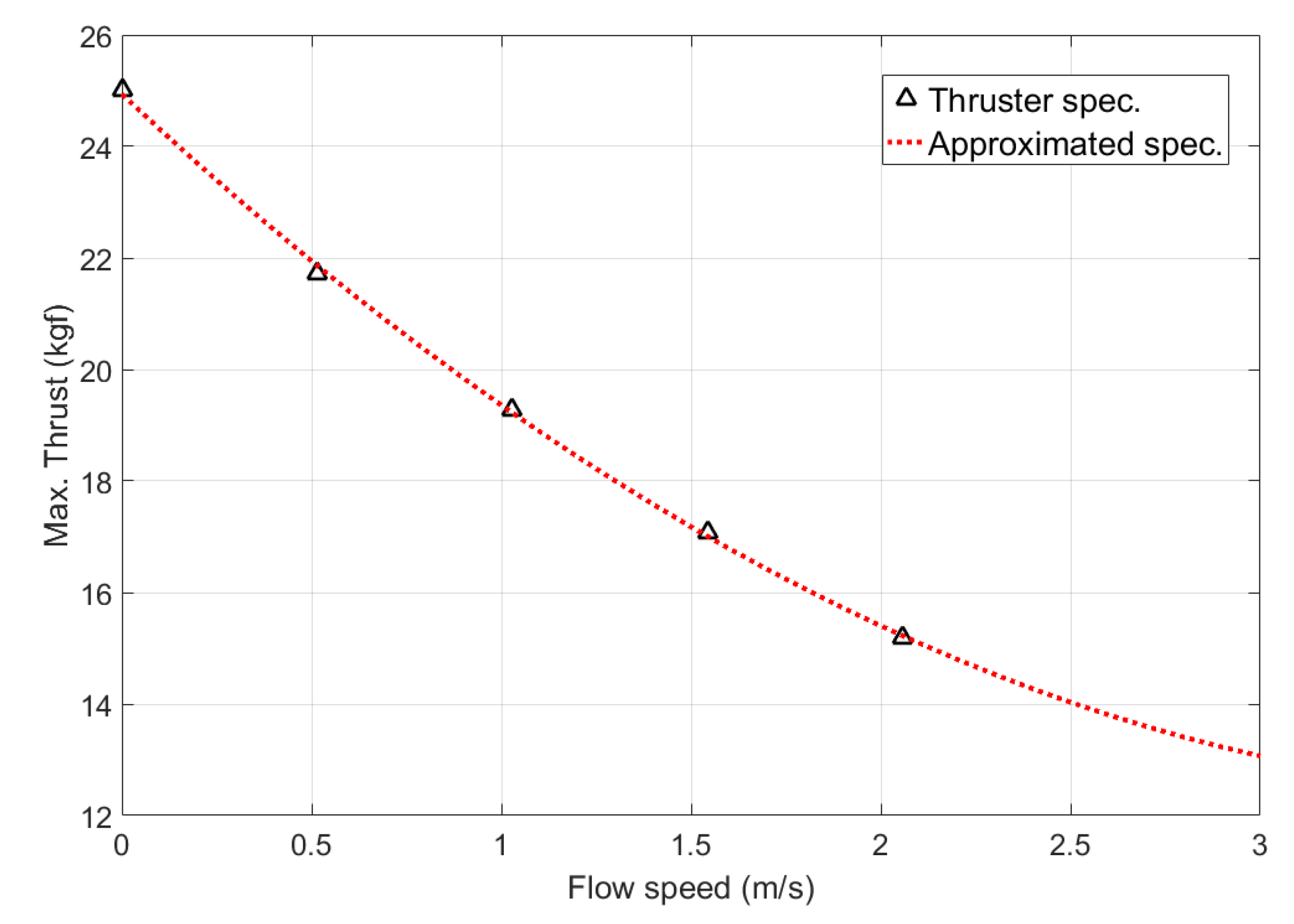
In the case of horizontal thrusters, the fact that the thruster’s maximum thrust force decreases in compliance with the increase of fluid speed flow through the thruster has to be considered.
According to the thruster’s specifications [13], the approximated relationship between the thruster maximum thrust force versus fluid flow speed (red dotted line in Figure 5) can be obtained as follows
F m a x ( U ) = g · ( 0 . 811 U 2 6 . 3903 U + 24 . 9384 ) ,
where F m a x denotes the maximum thrust force with the unit N, g = 9 . 8066 m/s 2 is the standard gravity, and U is the fluid speed flow through the thruster.
According to Figure 3, fluid speed for each of the four horizontal thrusters can be approximated using DVL measurement as follows
U H T f l U H T f r U H T b r U H T b l = 2 2 1 1 1 1 1 1 1 1 u v .
As mentioned before, the horizontal thruster has the same forward and reverse dynamics which can be expressed as follows
F H T ( x ) = F m a x ( U ) · s a t ( x / 5 ) .

4.5. Calculation of F c o n t r o l

Consequently, the control force F c o n t r o l in (6) can be calculated as follows
F c o n t r o l = 2 2 ( F H T f l + F H T f r + F H T b r + F H T b l ) 2 2 ( F H T f l F H T f r + F H T b r F H T b l ) F V T 1 F V T 2 F V T 3 F V T 1 R v c o s 15 F V T 2 R v c o s 45 F V T 3 R v s i n 15 F V T 1 R v s i n 15 + F V T 2 R v c o s 45 + F V T 3 R v c o s 15 R h ( F H T f l F H T f r F H T b r + F H T b l ) .

5. Simulation Studies

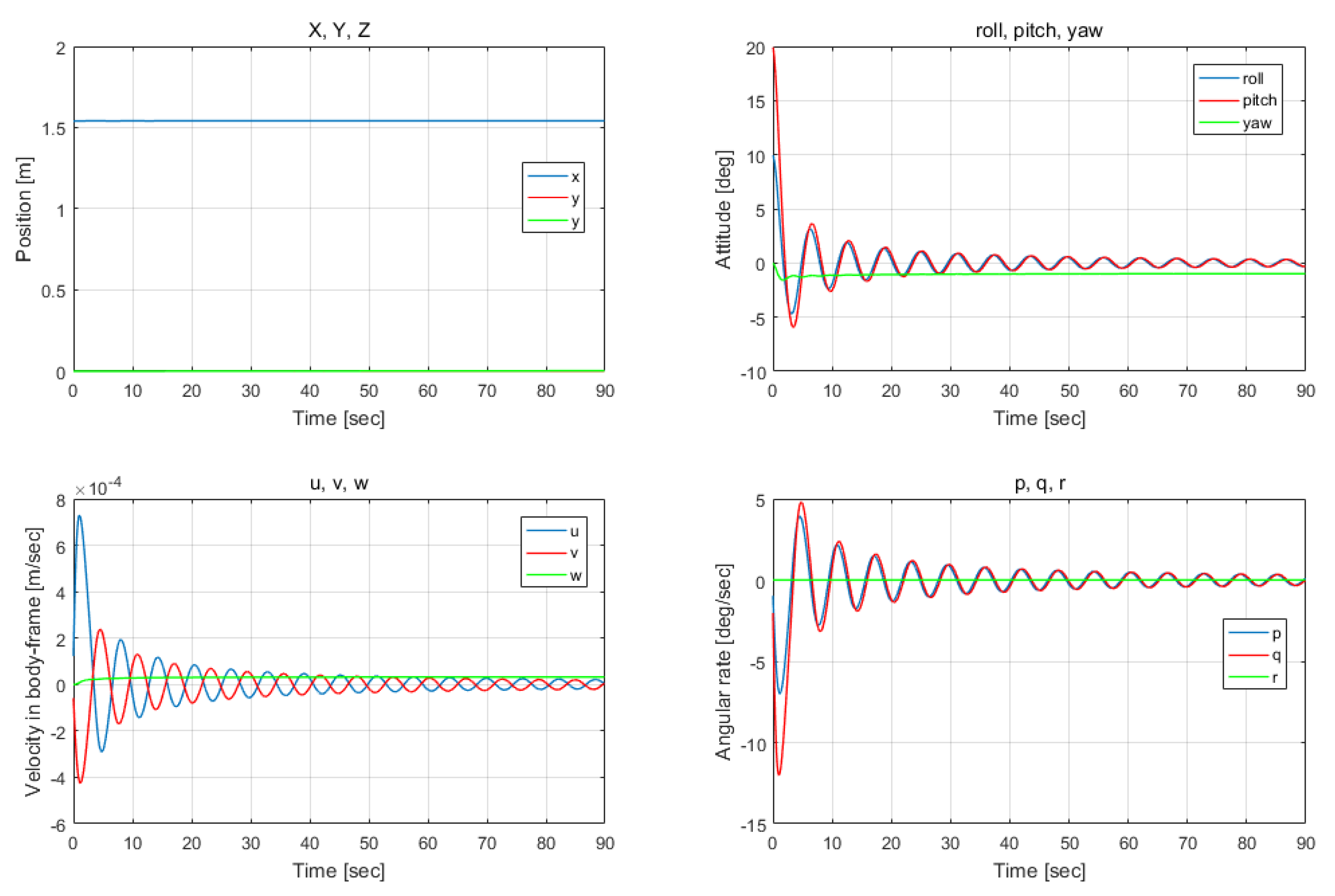
First, the vehicle’s platform stability on the horizontal plane is observed. The initial condition is set as η = [ 1 . 54 , 0 , 0 , 10 , 20 , 0 , 0 , 0 , 0 , 0 , 0 , 0 ] T , and simulation result is shown in Figure 6, from which it can be seen that the vehicle possesses suitable self-stability. Obviously, this kind of stability is caused by the fact that the vehicle’s gravity center is designed to be lower than the buoyancy center.
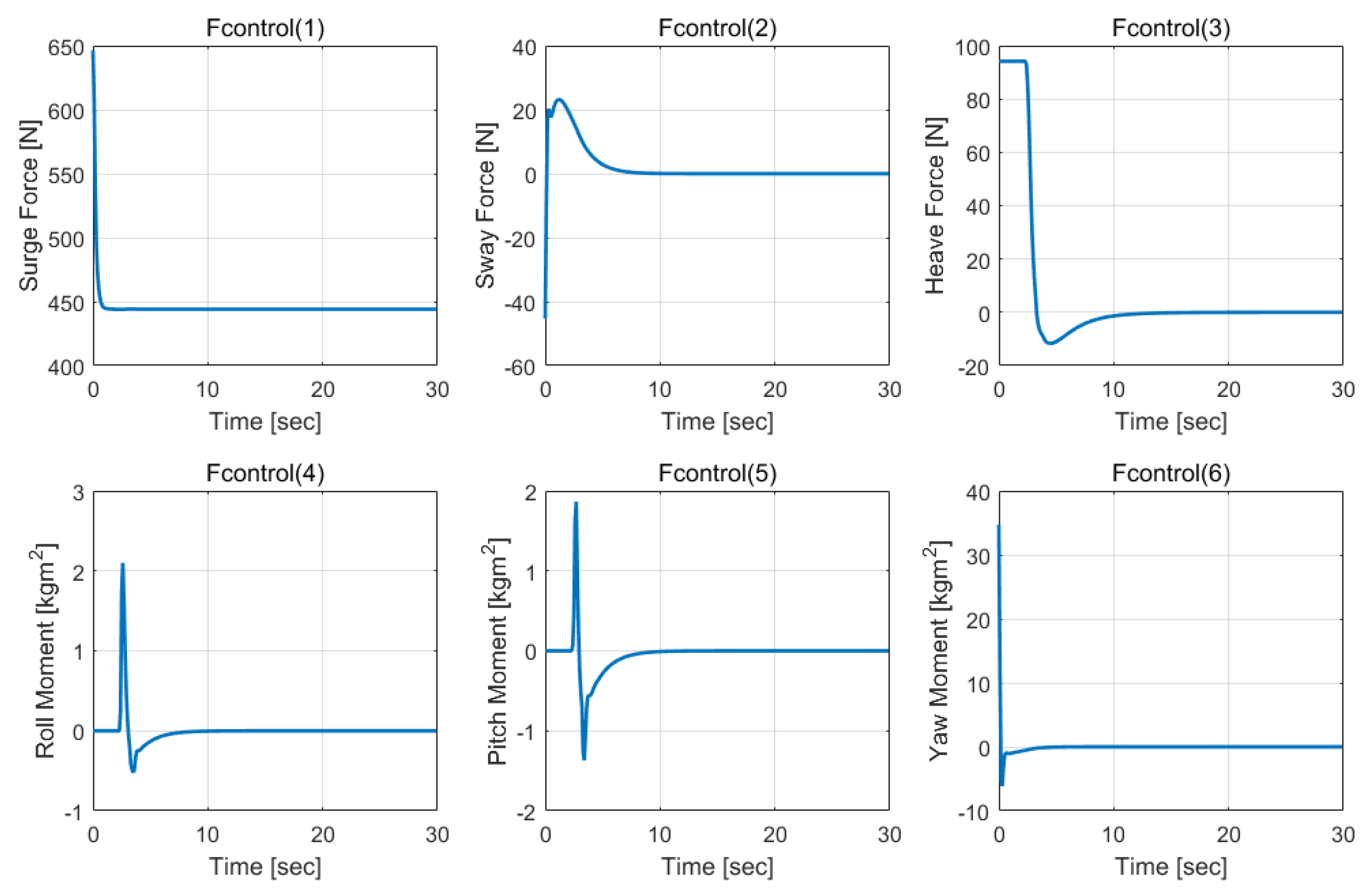
Then, it carries out the maximum forward speed simulation combined with the horizon and heading keeping tests. In the simulation, control gains are set as K v p = 5 , K v d = 10 , K v p d = 15 , K v d d = 45 , K h p = 2.5 , K h d = 3 , and other parameters are taken as ϕ r = θ r = 0 , ψ r = 30 , z r = 1.5 m , and sampling time is Δ T = 0.1 s . Figure 7 shows the control force F c o n t r o l 
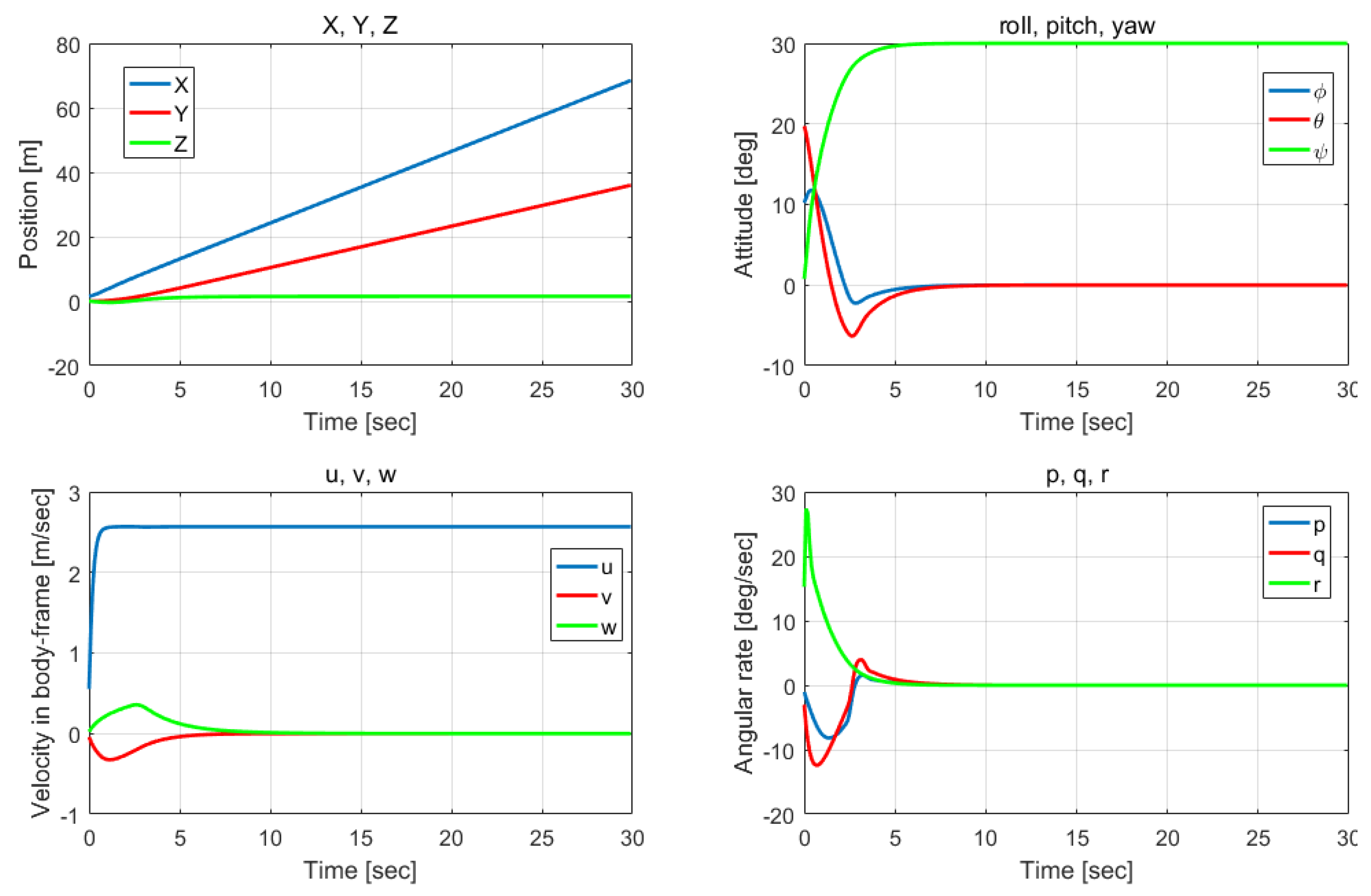
calculated using (38), and Figure 8 presents the corresponding vehicle motion information. From Figure 8, it can be seen that the vehicle’s maximum forward speed is about 2.56 m/s. This speed is lower than 3.2 m/s which is the simulation result in [28] where the effect of the relationship between the maximum thrust force and the fluid speed flow through the thruster was not considered. However, 2.56 m/s is still larger than the experimental result of 2.1 m/s, and this will be further discussed in the next section.

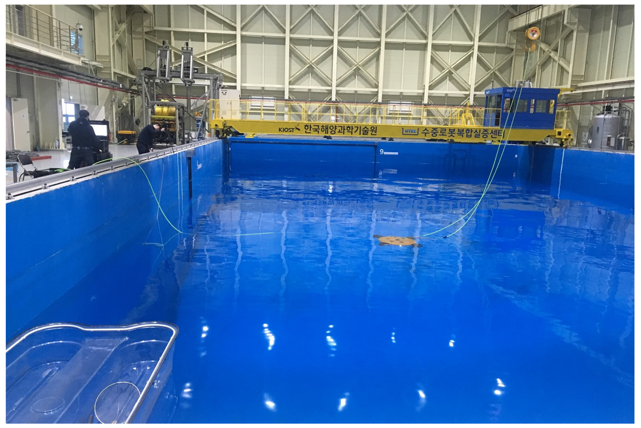
6. Experimental Studies

Experimental tests are carried out in the water tank and circulating water channel both in the Underwater Construction Robotics R&D Center (UCRC) in the Korea Institute of Ocean Science and Technology (KIOST) [29].
Figure 9 shows the engineering basin where the maximum forward speed test is taken. The experimental result is shown in Figure 10, from which it can be seen that the vehicle’s maximum forward speed is about 2.1 m/s. This speed is lower than the simulation result of 2.56 m/s. This might be caused by several reasons. One is that there are quite a number of coupled and complicated hydrodynamic terms that are not included in the vehicle’s model in the simulation. The second is that the drag component caused by the tether cable is not considered in the simulation. Indeed, this drag term might be significant in the case of the small size of underwater vehicles. From this point of view, whether the vehicle can be operated in AUV mode might be an important issue for the vehicle to overcome strong current. 
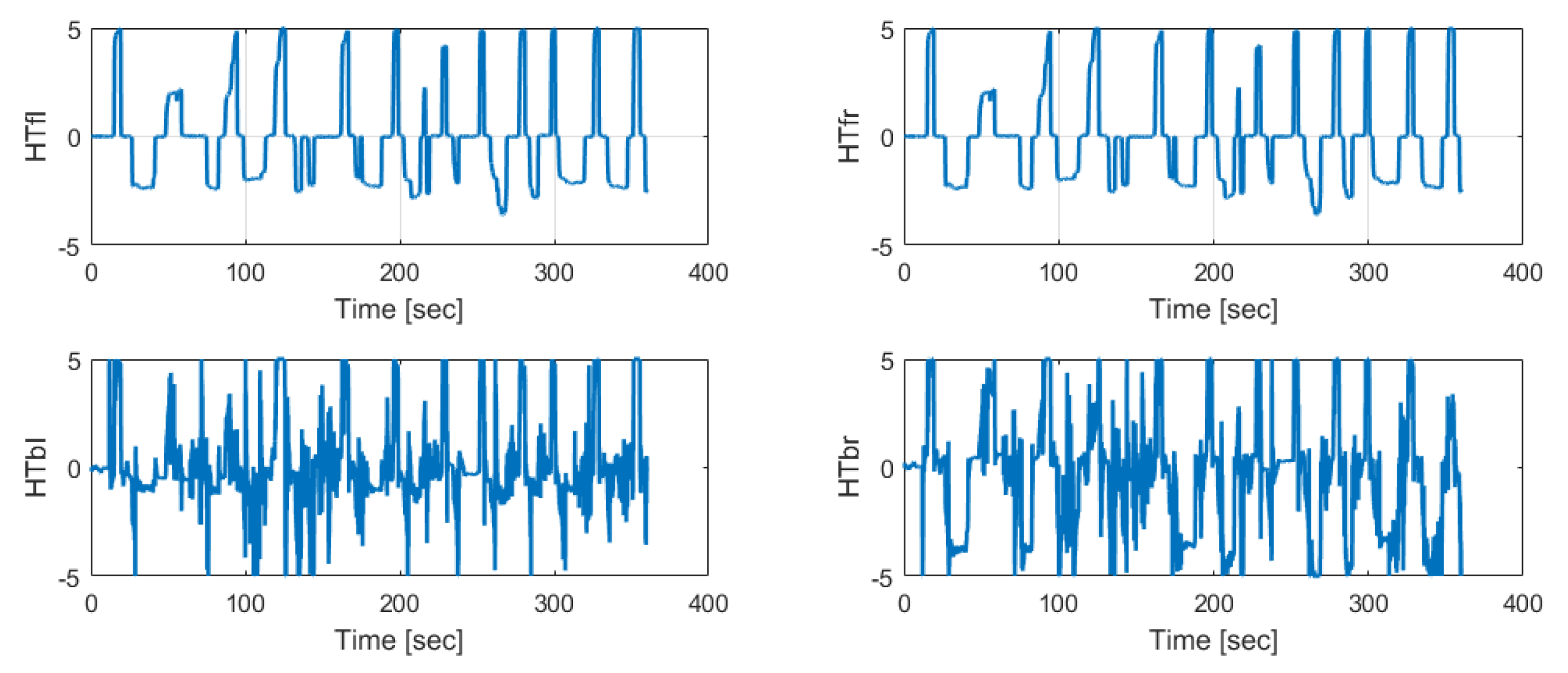
Figure 11 shows the control inputs for four of horizontal thrusters in this maximum forward speed test.
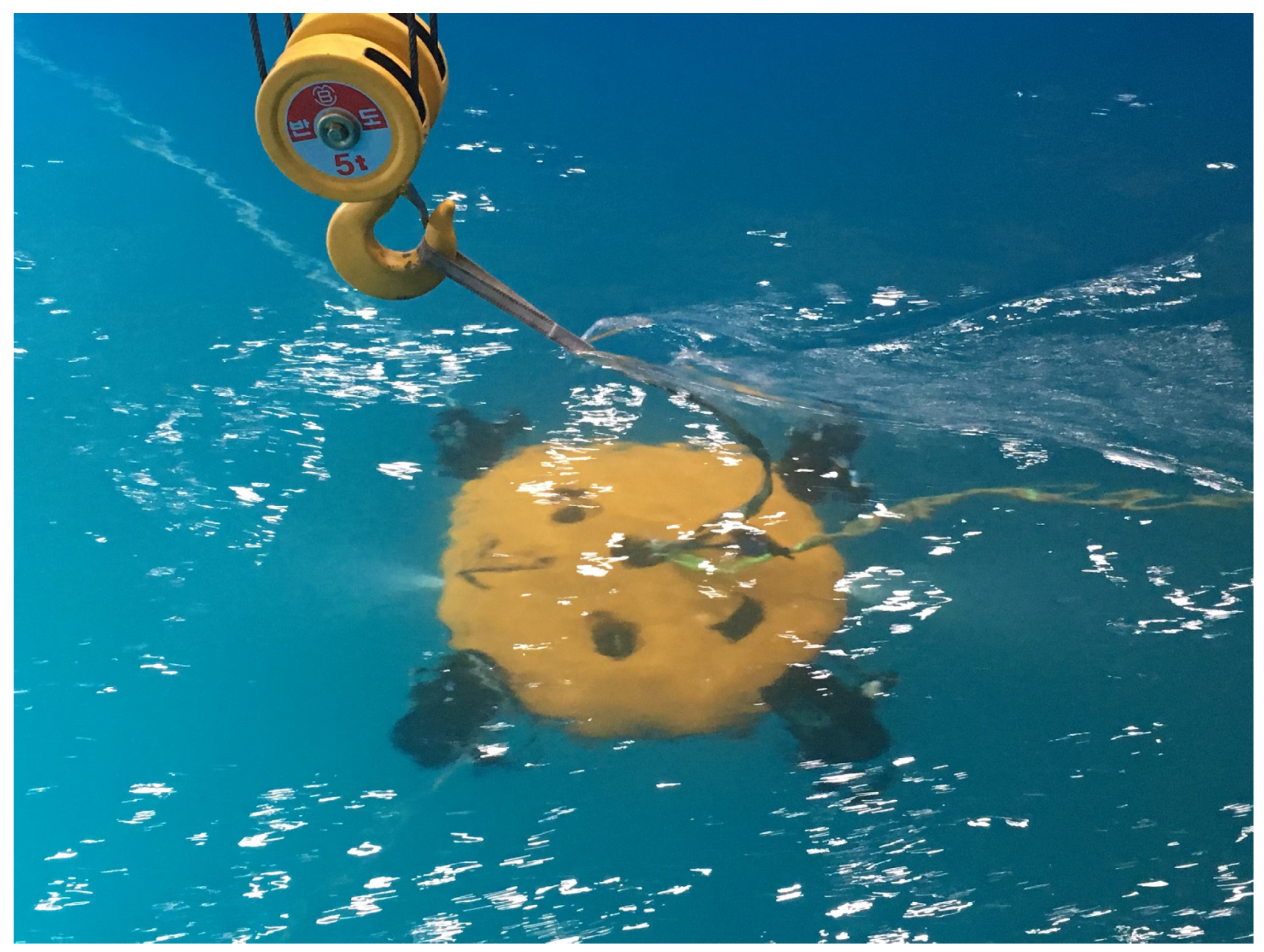
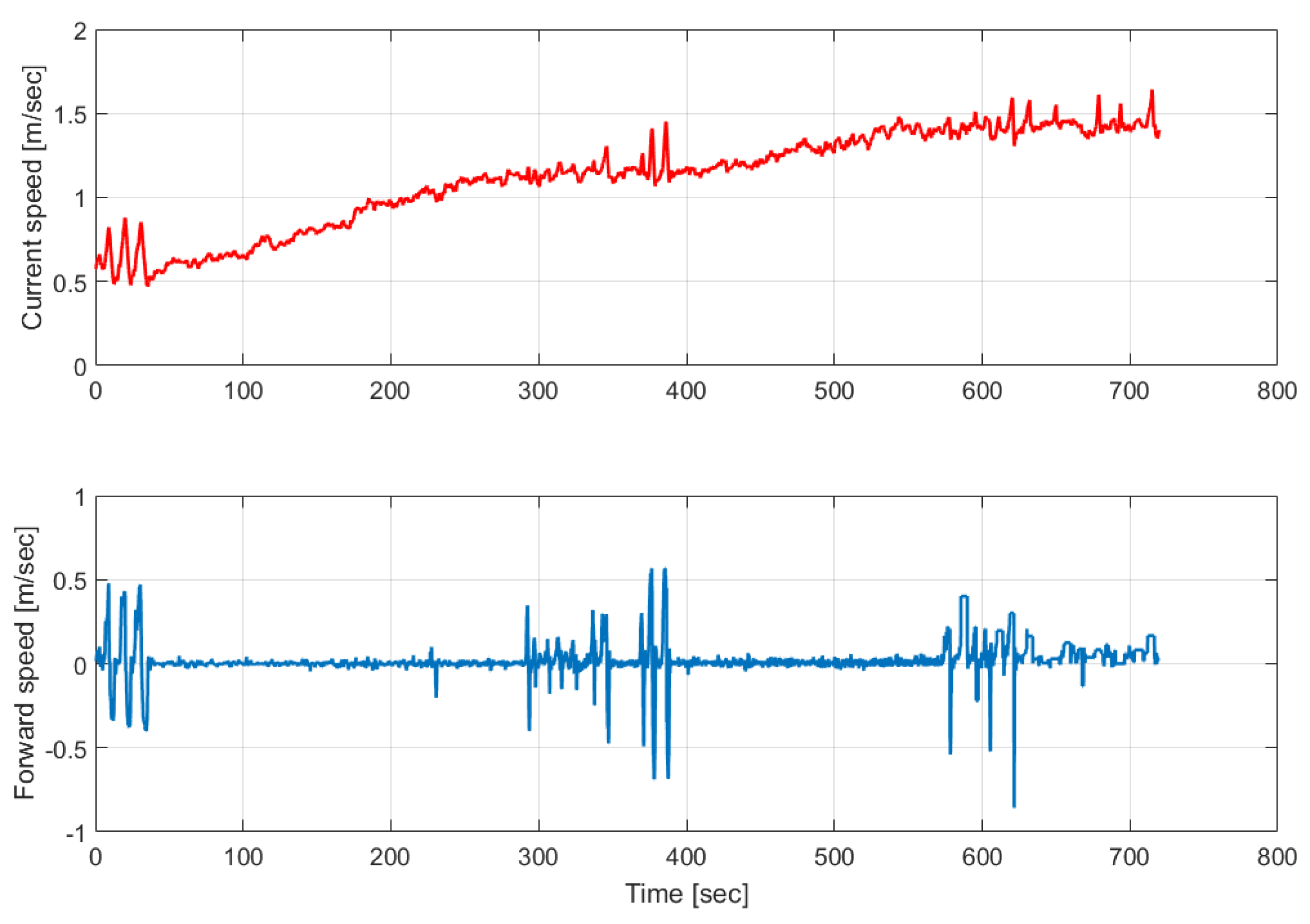
In addition, the test is taken where the vehicle is installed in the circulating water channel as in Figure 12, and it investigates if the vehicle can take the forward speed motion while keeping its heading in the strong current environment. In the test, the current speed is adjusted from 1.0 knots to 2.0 knots and further up to 2.5 knots. From the experimental result shown in Figure 13, it can be concluded that the vehicle can take forward motion even in the case where the current increased up to 2.5 knots.

7. Conclusions

This paper has presented the development of a UUV platform and its control method to overcome strong current. The vehicle has been designed to have a flattened ellipsoidal exterior to minimize the hydrodynamic damping. In addition, vectored thrust force control algorithm has been developed to maximize its horizontal speed. All of these technologies have been evaluated through both simulation and experimental tests. Especially, through the experimental studies carried out in the water tank and circulating water channel, it is found that, for the current version of vehicle platform, more strong roll and pitch moments might be needed to guarantee the vehicle’s horizontal stabilization.
During the next step of research works, the current version of the platform will be upgraded to have four vertical thrusters mounted symmetrically and each of the thrusters, similar to the horizontal thrusters, has the same forward and reverse dynamics. Moreover, each thruster will be more powerful compared to the current version and mounted more farther away from the center point. All of these are supposed to significantly increase the vehicle’s capability of stabilizing horizontal motion in the strong current environment.

Author Contributions

Conceptualization by J.-H.L.; methodology by J.-H.L., foremost, and then G.R.C. and M.-G.K.; software by H.K.; validation by M.-J.L. H.K. and M.-G.K.; formal analysis by G.R.C.; writing–original draft preparation by J.-H.L.; writing–review and editing by J.-H.L.; research supervision by J.-H.L. Authorship must be limited to those who have contributed substantially to the work reported.

Funding

This research was supported by the project titled “Development of Underwater Robot Platform and its Control Technology to Overcome up to 3.5 knots of Sea Current,” funded by the Ministry of Oceans and Fisheries (MOF) and Korea Institute of Marine Science and Technology Promotion (KIMST), Korea (20160148); It was also partially supported by the project No. 17-CM-RB-16 titled “Development of Multi-sensor Fusion based AUV’s Terminal Guidance and Docking Technology,” funded by the Agency for Defense Development (ADD) in the Korea.

Conflicts of Interest

The authors declare no conflict of interest.

References

  1. Hur, M.Y. Revisiting the Cheonan sinking in the Yellow Sea. Pac. Rev. 2017, 30, 349–364. [Google Scholar] [CrossRef]
  2. Kim, S.K. The Sewol Ferry Disaster in Korea and Maritime Safety Management. Ocean Dev. Int. Law 2015, 46, 345–358. [Google Scholar] [CrossRef]
  3. Sands, T.; Bollino, K.; Kaminer, I.; Healey, A. Autonomous Minimum Safe Distance Maintenance from Submerged Obstacles in Ocean Currents. J. Mar. Sci. Eng. Spec. Issue Intell. Mar. Robot. Model. Simul. Appl. 2018, 6, 98. [Google Scholar]
  4. Yoo, S.Y.; Shim, H.W.; Jun, B.H.; Park, J.Y.; Lee, P.M. Design of walking and swimming algorithms for a multi-legged underwater robot crabster CR200. Mar. Technol. Soc. J. 2016, 50, 74–87. [Google Scholar] [CrossRef]
  5. Pyo, J.H.; Yu, S.C. Development of AUV (MI) for strong ocean current and zero-visibility condition. In Proceedings of the IEEE AUV 2016 Conference, Tokyo, Japan, 6–9 November 2016; pp. 54–57. [Google Scholar]
  6. Eldred, R.A. Autonomous Underwater Vehicle Architecture Synthesis for Shipwreck Interior Exploration. Master’s Thesis, Department of Systems Engineering, Naval Postgraduate Scholl, Monterey, CA, USA, 2015. [Google Scholar]
  7. Bennett, S. A brief history of automatic control. IEEE Control Syst. Mag. 1996, 16, 17–25. [Google Scholar]
  8. Astrom, K.J.; Murray, R.M. Feedback Systems; Princeton University Press: Princeton, NJ, USA, 2008. [Google Scholar]
  9. Fossen, T.I. Marine Control Systems: Guidance, Navigation and Control of Ships, Rigs and Underwater Vehicles; Marine Cybernetics: Trondheim, Norway, 2002. [Google Scholar]
  10. Newman, J.N. Marine Hydrodynamics; The MIT Press: Cambridge, MA, USA, 1977. [Google Scholar]
  11. Prestero, T. Verification of a Six-Degree of Freedom Simulation Model for the REMUS Autonomous Underwater Vehicles. Master’s Thesis, Department of Ocean Engineering and Mechanical Engineering, MIT, Cambridge, MA, USA, 2001. [Google Scholar]
  12. Kim, J.; Chung, W.K. Accurate and practical thruster modeling for underwater vehicles. Ocean Eng. 2006, 33, 566–586. [Google Scholar] [CrossRef]
  13. Tecnadyne Technical Report. Available online: http://tecnadyne.com/wp-content/uploads/2017/06/Model-1040-Brochure-1.pdf (accessed on 18 May 2018).
  14. Lobo, K.; Lang, J.; Starks, A.; Sands, T. Analysis of Deterministic artificial Intelligence for Inertia Modifications and Orbital Disturbance. Int. J. Control Sci. Eng. 2018, 8, 52–62. [Google Scholar]
  15. Sands, T. Improved Magnetic Levitation via Online Disturbance Decoupling. Phys. J. 2015, 1, 272–280. [Google Scholar]
  16. Sands, T. Physics-Based Control Methods; Chapter in Advancements in Spacefraft Systems and Orbit Determination; InTech: London, UK, 2012; pp. 29–54. [Google Scholar]
  17. Fossen, T. Comments on ’Hamiltonian Adaptive Control of Spacecraft. IEEE Trans. Autom. Control 1993, 38, 671–672. [Google Scholar] [CrossRef]
  18. Nakatani, S.; Sands, T. Autonomous Damage Recovery in Space. Autom. Control Intell. Syst. 2016, 2, 23–36. [Google Scholar]
  19. Nakatani, S.; Sands, T. Battle-damage tolerant automatic controls. Electr. Electron. Eng. 2018, 8, 10–23. [Google Scholar]
  20. Sands, T.; Bollino, K. Autonomous Underwater Vehicle Guidance, Navigation, and Control; Chapter in Autonomous Vehicle; InTech: London, UK, 2019. [Google Scholar]
  21. Slotine, J.J.E.; Benedetto, M.D. Hamiltonian Adaptive Cotnrol of Spacecraft. IEEE Trans. Autom. Control 1990, 35, 848–852. [Google Scholar] [CrossRef]
  22. Sands, T.; Kim, J.; Agrawal, B. Improved Hamiltonian adaptive control of spacecraft. In Proceedings of the IEEE Aerospace Conference, Big Sky, MT, USA, 7–14 March 2009. [Google Scholar]
  23. Astrom, K.J.; Wittenmark, B. Adaptive Control; Addison Wesley Longman: Boston, MA, USA, 1995. [Google Scholar]
  24. Farrell, J.; Barth, M. The Global Positioning System and Inertial Navigation; McGraw-Hill, Two Penn Plaza: New York, NY, USA, 1996. [Google Scholar]
  25. Hong, S.; Lee, M.H.; Chun, H.U.; Kwon, S.H.; Speyer, J.L. Experimental study on the estimation of lever arm in GPS/INS. IEEE Trans. Veh. Technol. 2006, 55, 431–448. [Google Scholar] [CrossRef]
  26. Titterton, D.H.; Weston, J.L. Strapdown Inertial Navigation Technology; Peter Peregrinus Ltd.: London, UK, 1997. [Google Scholar]
  27. Tecnadyne Technical Report. Available online: http://tecnadyne.com/wp-content/uploads/2017/06/Model-300-Brochure-3.pdf (accessed on 18 May 2018).
  28. Li, J.H.; Kim, M.G.; Kang, H.; Lee, M.J.; Cho, G.R. Development of UUV platform and its control method to overcome strong currents: simulation and experimental studies. In Proceedings of the 11th IFAC Conference on Control Applications in Marine Systems, Robotics, and Vehicles, Opatija, Croatia, 10–12 September 2018; 2018. [Google Scholar]
  29. Kim, J.H.; Sitorus, P.E.; Won, B.R.; Le, T.Q.; Ko, J.H.; Kim, D.Y.; Jang, I.S. A flow-visualization study of a multiple hydrofoils duct with particle image velocimetry equipment in KIOST. In Proceedings of the 12th International Symposium on Particle Image Velocimetry, Busan, Korea, 18–22 June 2017. [Google Scholar]
Figure 1. Developed unmanned underwater vehicle (UUV) platform with the flattened ellipsoidal exterior.
Jmse 07 00089 g001
Figure 2. Motion sensor arrangement and lever arm coordinates for the developed vehicle: (a) is the motion sensor arrangement; and (b) shows the AHRS lever arm coordinates.
Jmse 07 00089 g002
Figure 3. Horizontal thrusters arrangement and maximum vectored horizontal thrust force.
Jmse 07 00089 g003
Figure 4. Vertical thrusters arrangement.
Jmse 07 00089 g004
Figure 5. Horizontal thruster’s specification: maximum thrust force vs. flow speed.
Jmse 07 00089 g005
Figure 6. Simulation result of self-stabilization capability.
Jmse 07 00089 g006
Figure 7. Calculated control forces in the maximum speed simulation.
Jmse 07 00089 g007
Figure 8. Vehicle’s motion information in the maximum speed simulation.
Jmse 07 00089 g008
Figure 9. Maximum forward speed test in the engineering basin.
Jmse 07 00089 g009
Figure 10. Experimental result of maximum forward speed with heading keeping.
Jmse 07 00089 g010
Figure 11. Control inputs for four of horizontal thrusters in the maximum forward speed test.
Jmse 07 00089 g011
Figure 12. The test in the circulating water channel.
Jmse 07 00089 g012
Figure 13. Vehicle’s forward motion test results in the circulating water channel.
Jmse 07 00089 g013
Table 1. Inertia Moments.
ParametersValueUnit
I x x 3.33 e + 000 kg·m 2
I y y 3.33 e + 000 kg·m 2
I z z 7.45 e + 000 kg·m 2
Table 2. Hydrodynamic Damping Coefficients.
ParametersValueUnit
X u | u | 6.74 e + 001 kg/m
Y v | v | 6.74 e + 001 kg/m
Z w | w | 5.38 e + 002 kg/m
K p | p | 3.73 e + 001 kg·m 2 /rad 2
M q | q | 3.73 e + 001 kg·m 2 /rad 2
N r | r | 6.92 e + 001 kg·m 2 /rad 2
Table 3. Added Mass Coefficients.
ParametersValueUnit
X u ˙ 1.75 e + 001 kg
Y v ˙ 1.75 e + 001 kg
Z w ˙ 2.09 e + 002 kg
K p ˙ 5.03 e + 000 kg·m 2 /rad
M q ˙ 5.03 e + 000 kg·m 2 /rad
N r ˙ 1.17 e + 000 kg·m 2 /rad

