1. Introduction
RF-based wireless communication is a vital tool for many industries. However, despite its prolific use for terrestrial applications, the effect of the maritime environment on RF propagation is still not well-characterized. An excellent listing of various factors that can affect RF propagation in the maritime environment is compiled in [
1]. These factors include weather, sea conditions and sea state, atmospheric effects, transmitter mobility, and the specifications of the wireless system employed. Clearly, RF propagation in a maritime environment is a highly multivariate problem.
In this paper, we study the real-world propagation of an RF system appropriate for near-shore unmanned surface vehicle operations. Example applications for near-shore surface vehicles include maritime search-and-rescue, disaster response, coral reef surveying, etc. These RF systems are typically deployed “ad hoc”, require high bandwidths (>20 Mb/s), low antenna heights (<5 m), and a strong receive signal strength (>−80 dBm) to ensure a reliable connection and to overpower ambient RF interference. For this reason, we chose the Ubiquiti Airmax wireless standard, which is designed to meet the needs of outdoor wireless local area networks (WLAN). We evaluate two systems, one system based on the 2.4 GHz frequency band, and one based on the 5 GHz frequency band; both of which are nearly ubiquitously legal to operate unlicensed worldwide. Previous research in maritime RF propagation compares measured received signal strength (RSSI) data to various loss models to evaluate the efficacy of an RF system in the maritime environment; however, these studies are typically only limited to RSSI data collection over water with a specific RF system configuration that cannot be directly compared to similar experiments over land by other authors. Since the effect of the maritime environment on RF propagation is so multivariate, these single-domain studies make it impossible to understand how RF propagation is impacted due to factors unique to the maritime environment versus factors related to a typical deployment of the RF system over land. To address this degeneracy, we isolate the effects of transmission over seawater on RF propagation in a maritime environment by collecting RSSI data from an ad hoc WLAN over land. Then, using the same system in essentially the same location, collect RSSI data over seawater. The differences in the RSSI data between the over-land and over-seawater deployments in the same maritime environment, allows us to isolate the factors related to differences in the RF system, and the factors related to a typical RF deployment over land. A short summary of the previous research most relevant to this work is listed below.
In Ref. [
1], a survey on previous references is maritime RF propagation was compiled; this information informed the previously mentioned list of factors affecting RF propagation in maritime environments. Most references in this work compared empirically gathered RF propagation data over water to various existing RF propagation models. These include the free space path loss (FSPL) model, irregular terrain model (ITM), international telecommunication union (ITU) family of models, log-normal or log-distance model, two ray ground reflection (two-ray) mode, and three-ray ground reflection (three-ray) models. Some references proposed modified versions of these existing models based on their analyses.
In Ref. [
2], RF propagation data was collected in the 5 GHz frequency band, with antenna heights of
and
over an antenna separation distance of 10 km. This study also investigated line-of-sight and non-line-of-sight measurements intended for operations near urban environments. This data was compared to the FSPL and two-ray propagation models. Results show that the two-ray model fits the data well for large scale path loss in line-of-sight condition. As distance increases, the data demonstrated a higher rate of signal attenuation.
In Ref. [
3], RF propagation data was collected in the 2.4 GHz frequency band, with antenna heights of
,
, over an antenna separation distance of 2 km. This data was compared to the two-ray and ITU-R P.1546 propagation models. Results show that the two-ray model fit the data well, but the ITU-R P.1546 model did not. Weather conditions and wave fluctuations were also considered to analyze the received power difference in detail.
In Ref. [
4], RF propagation data was collected in the 5 GHz frequency band, with antenna heights of
,
m, over an antenna separation distance of 3 km. This study also investigated line-of-sight and non-line-of-sight measurements intended for operations near urban environments. This data was compared to the log-normal propagation models. Results show that the log-normal propagation model fit the data well, with a path-loss exponent between 2.7 and 5.6. In addition, it was shown that small-scale measurements could be approximated by the Type I extreme value distribution function with location parameter and scale parameter values of −15.7 dB and 3.3 dB, respectively.
In Ref. [
5], RF propagation data was collected in the 5 GHz frequency band, with antenna heights of
,
, over an antenna separation distance of 10 km. This data was compared to the FSPL, two-ray, and three-ray propagation models. Results showed that the two-ray propagation model fits the data when inside the crossover distance of the two-ray model. Outside of the crossover distance, the three-ray path loss model, which considers a refracted wave the evaporation duct and the reflective wave considered in the two-ray model, is a better model.
In Ref. [
6], RF propagation data was collected in the 1.95 GHz frequency band, with antenna heights of
,
, over an antenna separation distance of 10 km. This data was compared to the FSPL, two-ray, and three-ray propagation models. This data was compared to the FSPL model. Results demonstrated a path loss of 40 dB/decade, which does not match the prediction made by the FSPL model. This was not noted in Ref. [
6], but this result supports the general consensus in the literature that the FSPL model (which drops off at 20 dB/decade) is only valid for antenna separation distances less than the cutoff distance. The 40 dB/decade path loss matches the prediction made by the two-ray model for the ranges studied. In addition, [
6] also noted that the mean standard deviation of the maritime data was 10.3 dB, which is notably lager than the 8 dB mean standard deviation typical for systems over land.
In Ref. [
7] RF propagation data was collected in the 968 MHz, 3.5 GHz, and 5.8 GHz frequency bands, with antenna heights of
,
, over an antenna separation distance of 5 km. This data was compared to the free-space and two-ray propagation models. Results showed that the two-ray propagation model best fit the data, except when in near proximity of the antennas, where the model was understandably broken due to the antenna gain aperture not being modeled in the near field, as well as additional reflections due to stiffs and high cliffs in the proximity of the shore.
In Ref. [
8] RF propagation data was collected in the 5 GHz frequency band, with antenna heights of
,
, over antenna separation distances of
. The unusually high antenna heights considered were the focus of this work. Results showed that placing the transmitter higher fits the free-space model more as there is more line of sight and diminished effect of the multipath fading. By contrast, the two-ray model fit the lower antenna heights better, even in no line of sight scenarios.
In Ref. [
9] RF propagation data was collected in the 412 MHz frequency band, with antenna heights of
,
, over antenna separation distances of
. This study is the most similar reference to the work in our paper, as it recorded data over land and seawater. The measured data over the sea demonstrated a mean path loss delta of 10 dB when transitioning from land to sea. Other interesting phenomena observed were: a 1.1 dB path loss for every meter of tide increase, which is consistent with the ITU-R P.526-7 path loss model, and a 1 to 2 dB of path loss during calm sea states, but 3 to 6 dB path loss in sea state 4 (approximately).
Based on these references, the most common propagation models for the study of maritime RF propagation are the FSPL model, and two-ray model. In reality, the FSPL is contained within the approximate two-ray model, as will be discussed in this paper. For the near-shore, low-antenna height, operational environments we studied, these models are the most relevant and are utilized for the analysis in this paper.
2. Materials and Methods
2.1. Path Loss Models
In this work, we aim to characterize the relationship between receive signal strength indication (RSSI) and distance between the transmitting and receiving antenna. The transmitting power of an access point is typically described in units of dBm, which is the ratio of the power in the signal referenced to 1 mW in a log10 scale. Conversion equations between the mW and dBm scales used in this work are given in Equation (1).
One convenient method of describing the radiated power of a transmitting access point is the equivalent isotropically radiated power (EIRP), which represents the power an isotropic antenna shall emit to produce the power observed in the direction of maximum antenna gain. The logarithmic formulation for EIRP is given in Equation (2).
where
is the access point transmitting power,
is the transmitting isotropic antenna gain, and
is the cable loss between the access point and antenna. In this work, we investigate the RSSI vs. range of a 2.412 GHz and 5.240 GHz WLAN system. The EIRP of these two systems were matched to ensure that the two systems would demonstrate reasonably similar RSSI vs. range results. Note that physically matching the EIRP of the two systems is not necessarily sufficient to normalize the range of the two different frequencies; however, it will generally ensure that the two systems produce RSSI within the same order of magnitude.
In this work, we investigate two different loss models; the free-space path loss (FSPL), and the two-ray ground reflection (two-ray) models. The FSPL model is based on the Friss transmission formula [
10]. This is given in Equation (3) [
11].
where
is the receiving power in mW,
is the transmitting power in mW,
is the transmitting antenna gain in mW,
is the receiving antenna gain in mW,
is the wavelength in m,
are generalized path losses in mW, and
is the distance between the two antennas in m. The path loss of any transmission model is defined as the ratio of the transmitting power,
, over the receiving power,
, i.e., the reciprocal of Equation (3) in the case of the FSPL model. Because the loss ratio is typically very large, it is conventionally described logarithmically in dBm. Solving Equation (3) for
, and describing the result logarithmically in dBm results in the FSPL model shown in Equation (4).
Note that transmitting power, , and antenna gains, and , are typically expressed in dBm. For brevity, Equation (4) expresses these variables in mW, and therefore, conversions between mW and dBm should be made using Equation (1), as appropriate.
The two-ray model considers the line-of-sight path assumed in the FSPL model, as well as a single path that is reflected off of the ground, based on the heights of the two antennas. The ground surface is characterized by a ground reflection coefficient, R. The full two-ray model is given in Equation (5) [
11].
where
is the height of the transmitting antenna in m,
is the height of the receiving antenna in m, and
is the ground reflection coefficient (unitless); reference Equation (3) for the remaining variable names. A ground reflection coefficient of
represents perfect ground reflection, and
represents zero ground reflection [
11,
12,
13].
It is common practice to approximate the two-ray path model given in Equation (5) using three piecewise approximation functions based on the distance from the transmitting antenna. This equation set is given in Equation (6) [
11].
In Equation (6),
is called the crossover distance, and is it defined in Equation (7).
There are important intuitions to be drawn from the piecewise two-ray approximation model in Equation (6). Firstly, the extent of region one is defined by the height of the transmitting antenna, which is usually small relative to the total operating range of the wireless system. As such, region one is typically of little concern to researchers since its relevant range is very close to the transmitting antenna, on the order of meters. Secondly, the extent of region two is defined between region one and the crossover distance in Equation (7). In this region, the two-ray approximation model is identical to the FSPL model given in Equation (4), and power falls off at −20 dB/decade. Thirdly, region three consists of everything outside of the crossover distance. In this region, power falls off at −40 dB/decade.
In this work, the measured RSSI data is compared against the full, and approximate two-ray models, assuming that a generalized path loss variable, , is introduced into the real data. We hypothesize that the transition from over-land to over-seawater will manifest as an increase to this path loss variable.
Employing both the approximate and full version of the two-ray model is beneficial because the approximate two-ray model is useful for identifying path loss, whereas the full two-ray model also captures the constructive-destructive interference effect of ground reflection, and varying antenna heights. Because the RSSI data was collected with equivalent antenna heights for all experiments, fitting the data to the full two-ray model should enable us to observe a change in ground reflectivity in the transition from over-land to over-seawater. In addition, the approximate two-ray model is more commonly cited in preceding literature (e.g. Ref. [
1,
2,
3,
5,
14,
15]), which is important to note when drawing comparisons between our work and previous literature.
2.2. Experiment Description
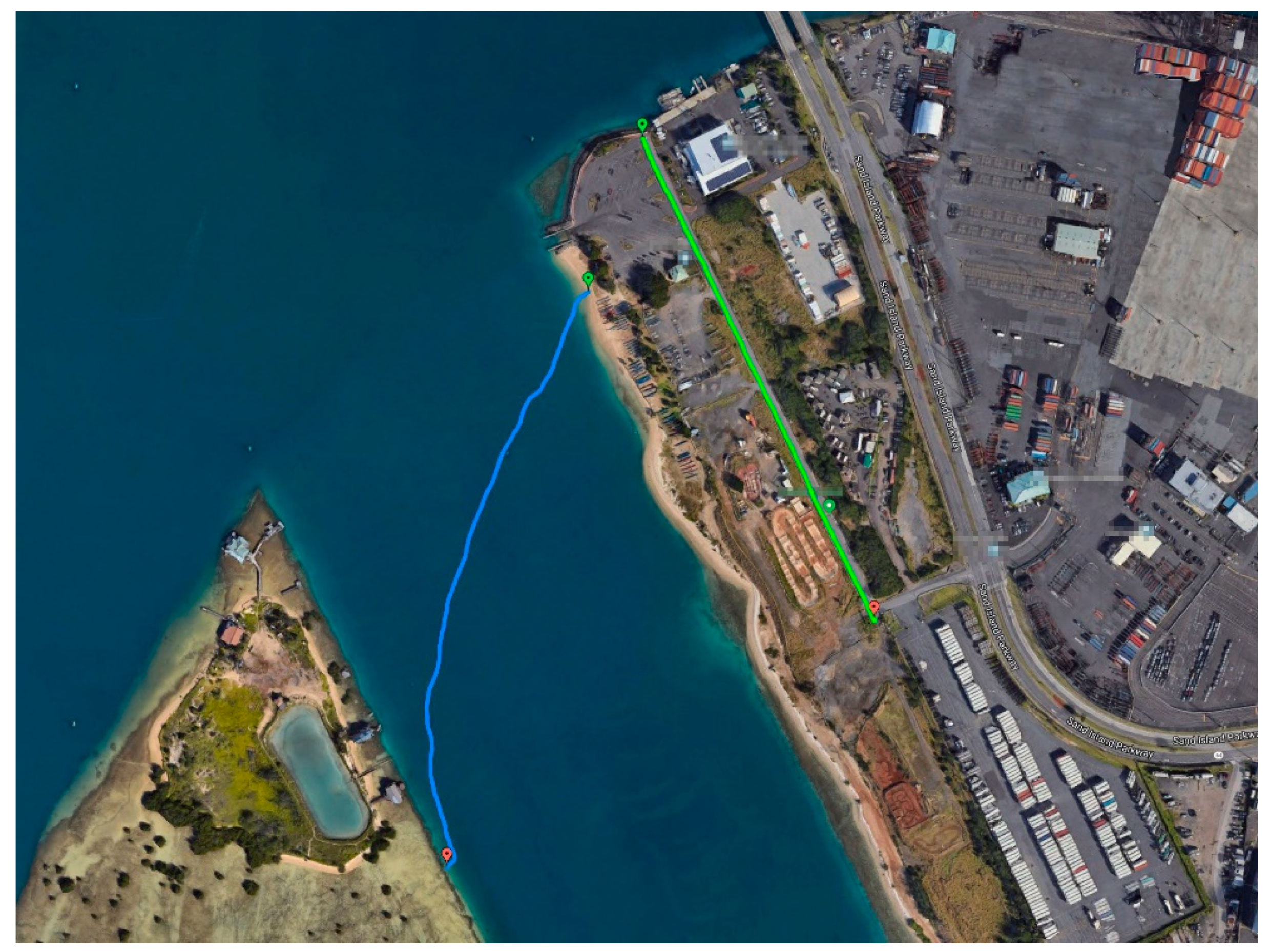
We selected the Sand Island Boat Launch Facility, located in Oahu, Hawaii, as the location for this study. This location is well suited for this experiment because it has a flat, approximately 0.5 km long entrance road with full line of sight. The over-land experiments were conducted on this entrance road, and the over-seawater experiments were conducted from the beach over the Sand Island channel. The two ground stations/origin points for each experiment were within 150 m of each other. The approximate over-land and over-seawater propagation paths are shown in
Figure 1.
Data were collected on two different days: 27 July 2019, and 15 August 2019. The protected nature of the Sand Island channel demonstrated a Beaufort Sea state of one (rippling waters and light air) for both days of testing. The height of the transmitting and receiving antennas was set based on the height of the seawater surface at the time of testing. At this location, the tide can fluctuate between from 0 m to 0.6 m over a period of roughly 6 h. Data collection over seawater lasted no more than 2 h on either day, resulting in a maximum error of 0.2 m in height due to shifting tides.
The Sand Island access road contains an occasional passing vehicle, and the Sand Island channel contains the occasional passing small boats or jet skis. During the experiment, if a passing car or vessel obstructed the line-of-sight between the transmitting antenna on the ground station and the receiving antenna on the mobile station, the data collection was paused, preventing those points from being recorded.
Two WLAN frequency bands were tested in this experiment, 2.4 GHz and 5 GHz. Note that the names “2.4 GHz” and “5 GHz” do not refer to the exact frequency employed, rather, they refer to the family of standardized IEEE 802.11 wireless channels, which specifies center frequency and bandwidth. The Airmax WLAN protocol used in this experiment adopts the IEEE 802.11 channel specification. Specific details about each system are listed in
Table 1.
The settings and equipment were identical for the transmitting and receiving ends of each RF system. The selected access point model (Ubiquiti BulletAC-IP67) is equipped with both 2.4 GHz, and 5 GHz transmitters, allowing us to test both frequencies while eliminating any variability due to differences in the access point hardware.
The RSSI data was recorded directly from the Ubiquiti dashboard software. This software runs on the computer connected to the access point. Because this dashboard software does not feature a RSSI data logging feature, we developed a JavaScript program to “scrape” and timestamp the relevant RSSI data from the dashboard back end at 1s intervals. This program and its development can be found at the GitHub repository [
17], or in the
Supplementary Materials.
The separation distance between the two antennas was measured using a global navigation satellite system (GNSS) sensor mounted to the stationary transmitting antenna ground station, and a second GNSS sensor mounted to the receiving antenna mobile station. The Adafruit Ultimate GPS was the selected GNSS sensor; this was connected to a laptop computer was running the Robot Operating System (ROS) Melodic Morenia software. The ROS package “nmea_navsat_driver” [
18] was used to communicate with the GNSS sensor. ROS features a message data logging service known as “bags” [
19], which was used to log and timestamp the GNSS sensor data. This bag file was later converted to a comma separate value (.csv) file for post-processing. For details on reproducing the GNSS data collection process, see Ref. [
17], or the
Supplementary Materials.
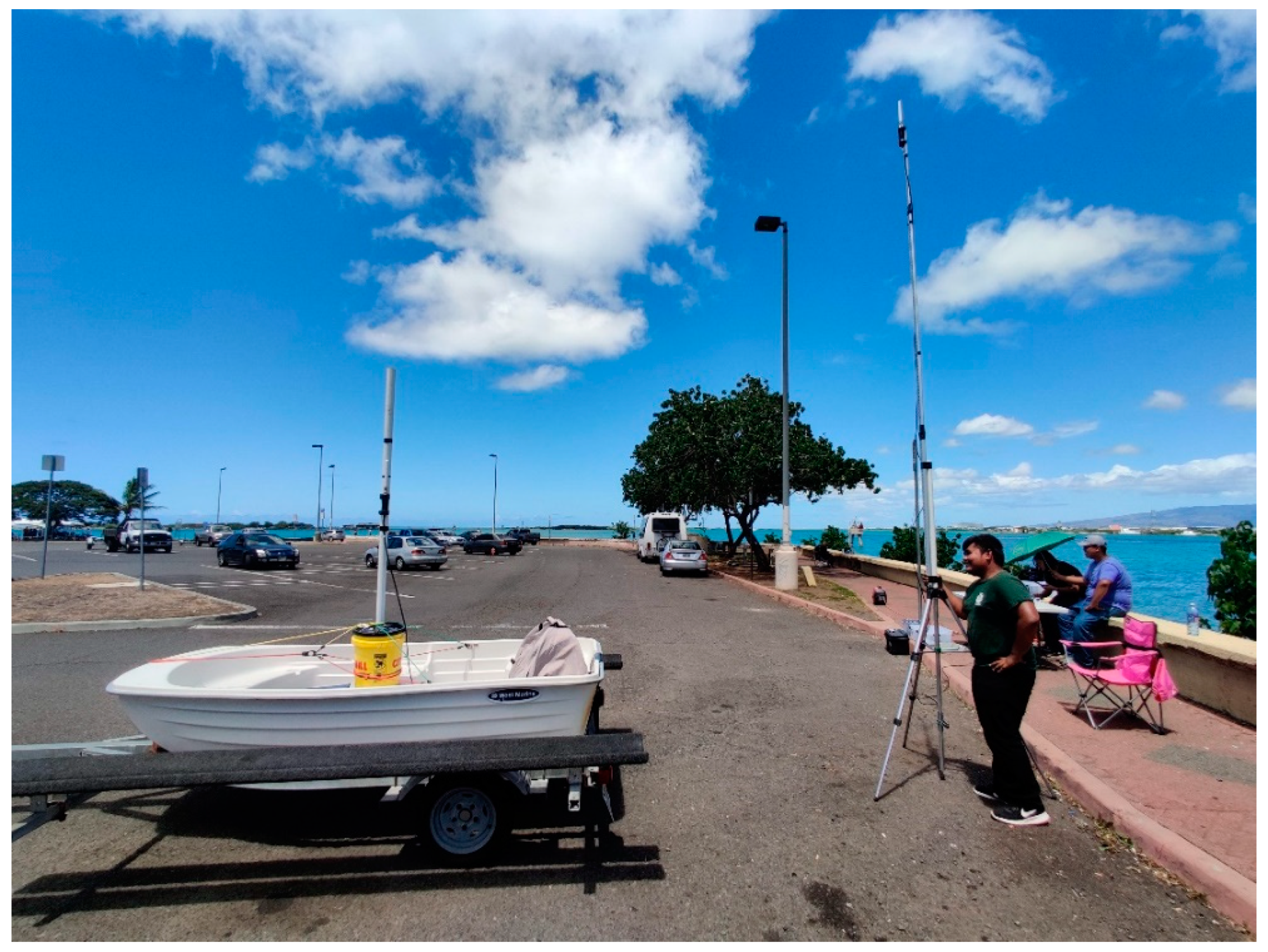
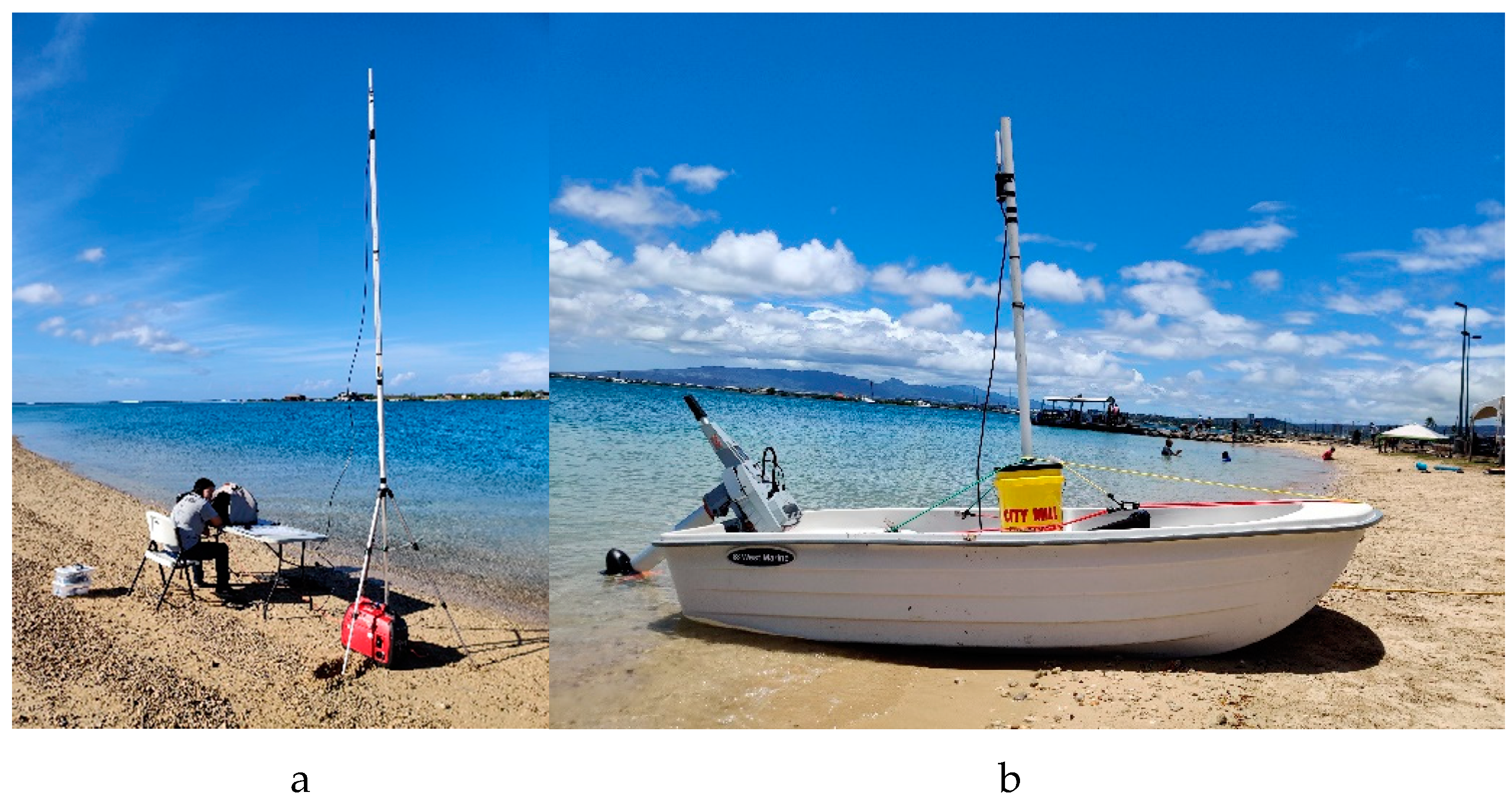
During the experiment, the transmitting antenna was located at the stationary ground station, and was mounted to a leveled tripod with a height-adjustable boom between 2 and 5 m. The receiving antenna was set to a fixed height of 2 m, and rigidly connected to the mobile station, which represents a robot. The mobile station comprised of a 9’4” rigid tender, which was pulled on a trailer during the over-land experiments, and manually driven using an outboard transom motor during the over-seawater experiments. An image of the ground station, transmitting antenna, mobile station, and receiving antenna for the over-land experiments is shown in
Figure 2. A pair of images of the ground station, transmitting antenna, mobile station, and receiving antenna for the over-seawater experiments is shown in
Figure 3.
3. Results
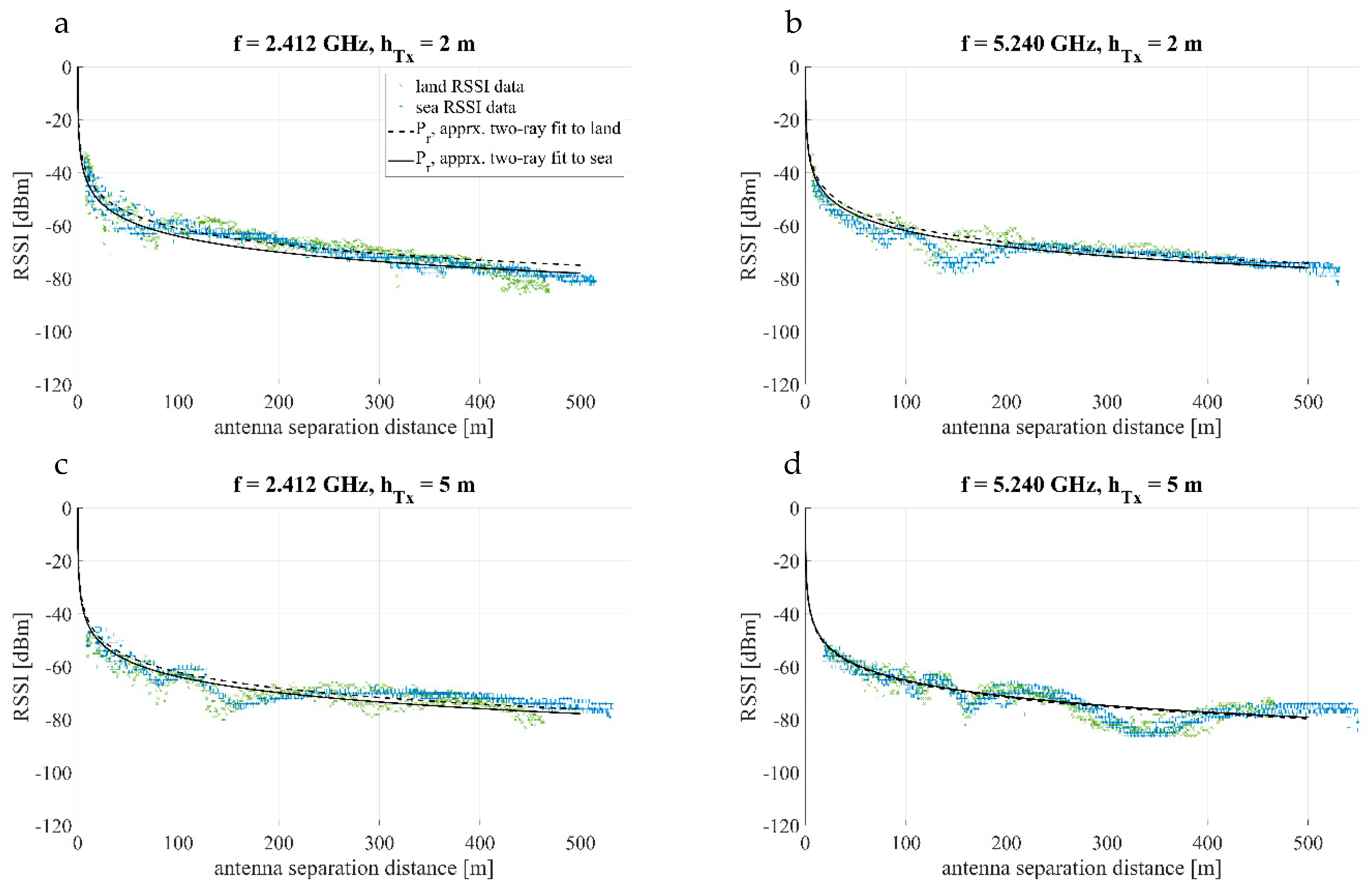
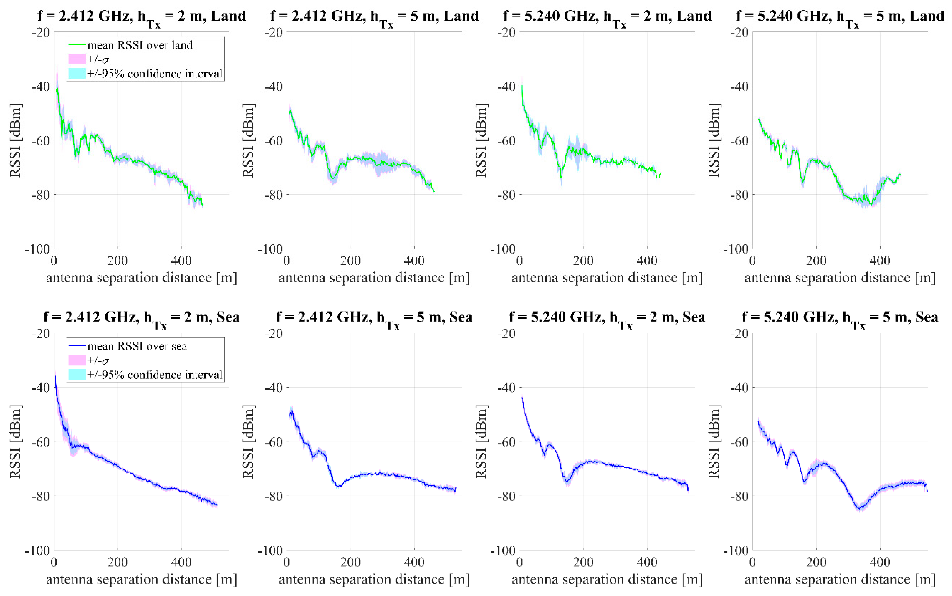
The collected RSSI measurements are plotted against distance in
Figure 4. In all experiments, the receiving antenna height was set to
. The transmitting antenna height was set to two different heights,
, and we evaluated two different WLAN frequencies,
. All of the collected RSSI data is shown in
Figure 4.
A statistical analysis of the binned mean, standard deviation, and confidence interval can be found in
Appendix A.
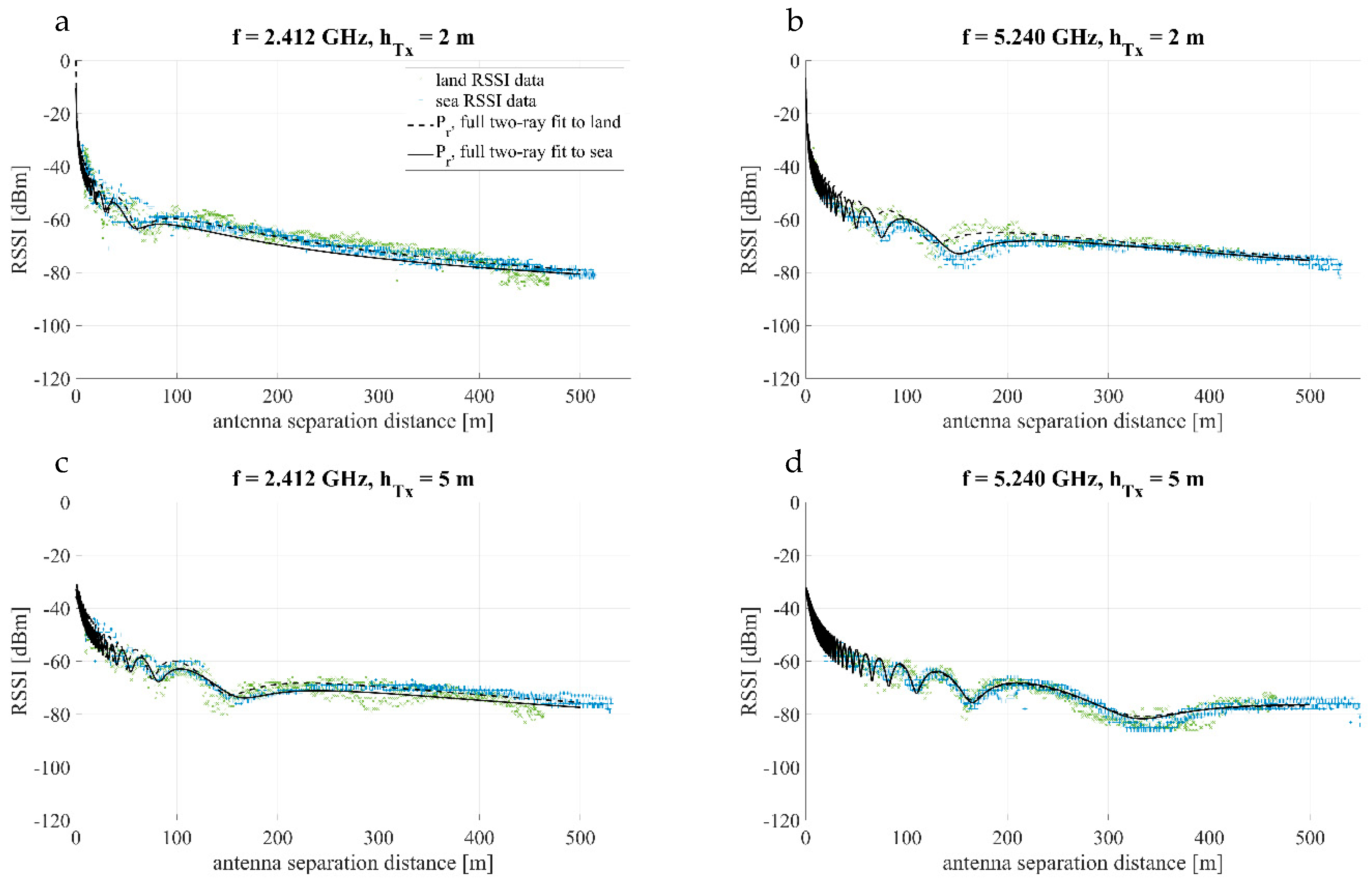
The measured RSSI data is plotted against three theoretical path loss curves in
Figure 5. These are:
The full two-ray path loss model from Equation (5)
The approximate region-two, two-ray path loss model (). This is identical to the free space path loss model
the approximate region-three, two-ray path loss model (). The respective frequencies and transmitting antenna heights are labeled in their respective subplots.
The theoretical path loss models plotted in
Figure 5 demonstrate significant deviation from the measured RSSI data; this is expected since the theoretical models assume ideal power transmission, geometry, and ground reflectivity. In the case of the approximate two-ray models, there is an additional path loss variable,
, demonstrated by a constant power difference between the models and true data. In the case of the full two-ray model, there is a path loss variable,
, demonstrated by a constant power difference between the model and true data; a non-ideal ground reflection coefficient,
, demonstrated by the decreased amplitude of the constructive-destructive interference pattern; and small variations in the transmitting antenna height,
, demonstrated by the difference in the frequency of the constructive-destructive interference pattern. To characterize these coefficients, we fit the approximate two-ray model, and full two-ray model classes to the real data using a least squares minimization against these characteristic coefficients.
As discussed in Equation (6), the approximate two-ray model consists of three piecewise approximations, which are defined as a function of distance. The boundary between the first and second region is defined by the transmitting antenna height,
, which is negligible in this case due to the short antenna height. The boundary between the second and third region is defined by the crossover distance,
, defined by Equation (7). These crossover distances are listed in
Table 2.
In all of the experiments except for the 2 GHz, 2m experiment, the crossover distance is greater than the maximum distance for which measurements were taken. Therefore, the region-two, two-ray model in Equation (6) is the most appropriate approximation for this data. In the 2 GHz, 2m experiment, the approximate region-two, two-ray model was only fitted to data before the 404 m crossover distance.
In
Figure 6, we fit the approximate region-two, two-ray model to all of the measured RSSI data. Because the only unknown variable in the approximate region-two, two-ray model is path loss,
, a single-variable least squares minimization against path loss,
, was sufficient to fit the theoretical model to the data.
The fitted coefficients from the approximate region-two, two-ray model are compiled in
Table 3.
The path loss difference when transitioning from over-land to over-seawater for each experiment is compiled in
Table 4.
The approximate two-ray model path loss deltas compiled in
Table 4 shows that the 2.4 GHz, 2 m experiment demonstrates a 3 dBm increase in path loss when transitioning from over-land to over-seawater; the 2.4 GHz, 5 m, and 5 GHz, 2 m experiments demonstrate a 1.7 dBm path loss when transitioning from over-land to over-seawater; and the 5 GHz, 5 m experiment demonstrates a 0.5 m
decrease in path loss when transitioning from over-land to over-seawater. This indicates that a combination of higher antenna height and frequency contribute to reduced path loss when transitioning from over-land to over-seawater.
In
Figure 7, we fit the full two-ray model to all of the measured RSSI data. In the full two-ray model, the path loss,
, ground reflection coefficient,
, and exact transmitting antenna height,
, are unknown and/or sensitive variables; therefore, a constrained multi-variable nonlinear least squares minimization against
,
, and
, was used to fit the theoretical model to the data.
was constrained to vary over the range
dBm,
over the range,
, and
over the range
m for the 2 m antenna experiments, and
m for the 5 m antenna experiments. As a general rule, the path loss varies the height of the curve on the y-axis, the transmitter antenna height varies the frequency of the constructive-destructive interference pattern, and the reflection coefficient varies the amplitude of the constructive-destructive interference pattern.
The fitted coefficients from the full two-ray model are compiled in
Table 5.
The path loss difference when transitioning from over-land to over-seawater for each experiment is compiled in
Table 6.
The full two-ray model path loss deltas compiled in
Table 6 demonstrate similar results to the approximate two-ray model path loss deltas given in
Table 4, except for the 2.4 GHz, 2 m experiment, where the full two-ray model demonstrated a 2 dBm path loss delta, compared to the 3 dBm path loss delta of the approximate two-ray model. Inside the cutoff distance,
, where the RSSI decreases at a rate of roughly 20 dBm/decade, a path loss of 2 dBm results in an overall range decrease of 26%, and a path loss of 3 dBm is roughly equivalent to an overall range decrease of 41%. Because the 5 GHz 5 m experiment does not demonstrate this path loss, the combination of the higher 5 GHz frequency band in combination with 5 m transmitting antenna height results in a substantially smaller path loss over seawater.
Regarding ground reflection coefficient,
, the full two-ray model demonstrated a relatively constant
over the four different over-land experiments (2 GHz, 2 m; 2 GHz, 5 m; 5 GHz, 2 m; 5 GHz, 5 m); however,
changed significantly over the four different over-seawater experiments. The 2 GHz, 2 m experiment demonstrated
; the 2 GHz, 5 m experiment demonstrated
; the 5 GHz, 2 m experiment demonstrated
; and the 5 GHz, 5 m experiment demonstrated
. These results indicate that the R, as described in Equation (5) in [
11], is constant when operating over land, but varies with frequency when operating over seawater. Because the ground reflection coefficient affects the amplitude of the constructive-destructive interference pattern inside the cutoff distance, a large
can result in large changes in RSSI over relatively short distances; however, it does not have a significant effect on the overall “range” of the wireless system, especially when the antenna separation distance approaches and exceeds the cutoff distance.
4. Discussion
In this work, we studied the received signal strength indication (RSSI) of 2.4 GHz and 5 GHz wireless local area network (WLAN) systems over land and seawater, using transmitting antenna heights of
= {2, 5} m, with a maximum antenna separation distance of 0.5 km. We fit these measurements to the approximate two-ray propagation model (also called the free space path loss model) and the full two-ray path loss model. Results showed that the 2.4 GHz system demonstrated an increase in path loss of 2 to 3 dBm when transitioning from over-land to over-seawater for both antenna heights; in practice, a 2 to 3 dBm path loss is equivalent to reduction of 25-40% in range for a WLAN. Interestingly, the 5 GHz system with a 5m transmitting antenna height did not demonstrate any significant change in path loss when transitioning from over-land to over-seawater. Therefore, if all other variables are equal, given the choice between the 2.4 GHz and 5 GHz frequency bands for near-shore, WLAN operations, the 5 GHz frequency band coupled with an antenna height of roughly 5 m will minimize the path loss penalty of operating over seawater, which also indicates future near-shore unmanned systems designers can expect accurate range predictions from 5 GHz, 5 m systems in practice. To the authors’ knowledge, no other work prior has demonstrated this difference in path loss delta between 2.4 GHz and 5 GHz systems. Because only two frequencies were tested in this work, it is dangerous to extrapolate this assumption for all frequencies; however, previous work in [
9] demonstrated a 10 dBm loss when transitioning from over-land to over-seawater for a 412 MHz system; this result weakly agrees with our experiment.
In addition, we also investigated the effect of the ground reflection coefficient,
, by fitting the full two-ray path model given in Equation (5), to the collected data. We found that
remained relatively constant (
) for all of the over-land experiments; however,
changed significantly over the four different over-seawater experiments. The 2 GHz, 2 m experiment demonstrated
; the 2 GHz, 5 m experiment demonstrated
; the 5 GHz, 2 m experiment demonstrated
; and the 5 GHz, 5 m experiment demonstrated
. These results indicate that the
, as described in Equation (5) in [
11], is constant when operating over land, but varies with frequency when operating over seawater.
is generally considered to be a function of the antenna polarization direction, the angle of incidence with the ground,
, and the relative complex permittivity of the land and/or seawater surface,
[
11,
13]. In particular the
of a medium depends slightly on frequency because of the Debye-Falkenhagen effect; however, this effect is generally considered to be negligible [
20], and does not account for the significant change in
measured in this work. Previous work also suggests that the form of the constructive-destructive interference pattern is sensitive to sea-surface roughness, and the refraction of the propagating waves [
21,
22]; which may account for this discrepancy.
In future work, one should focus on models explaining why the 2.4 GHz frequency band demonstrates a greater path loss than the 5 GHz frequency band when transitioning from over-land to over-seawater. The approximate two-ray/free space and full two-ray models can be fitted to real data to describe this path loss; however, these models are currently insufficient to predict this phenomena. In addition, the ground reflection coefficient, , also demonstrated a frequency dependence that is not predicted by current models. A similar experiment involving more frequencies should better describe the nature of this frequency dependence.

 ,
, 


