
A Data-Driven Method for Ship Motion Forecast
Abstract
:1. Introduction
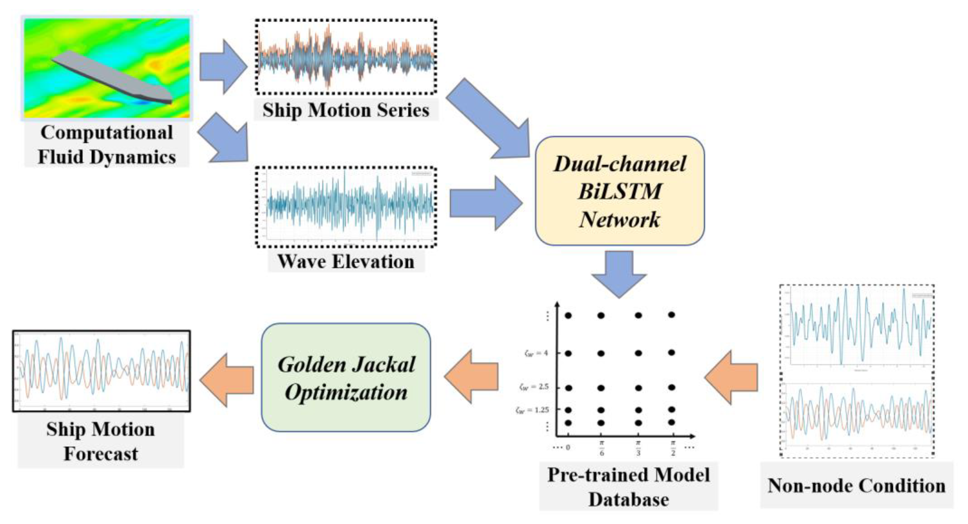
2. Methods
2.1. Ship Motion Response Model
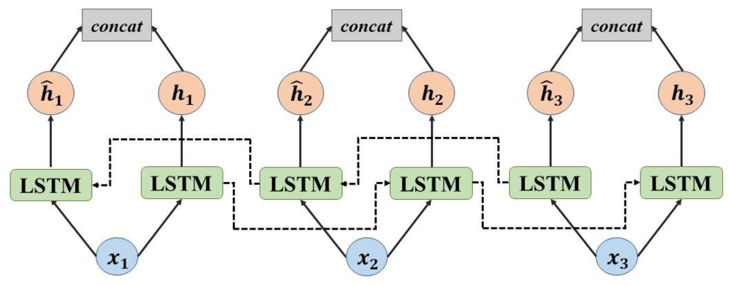
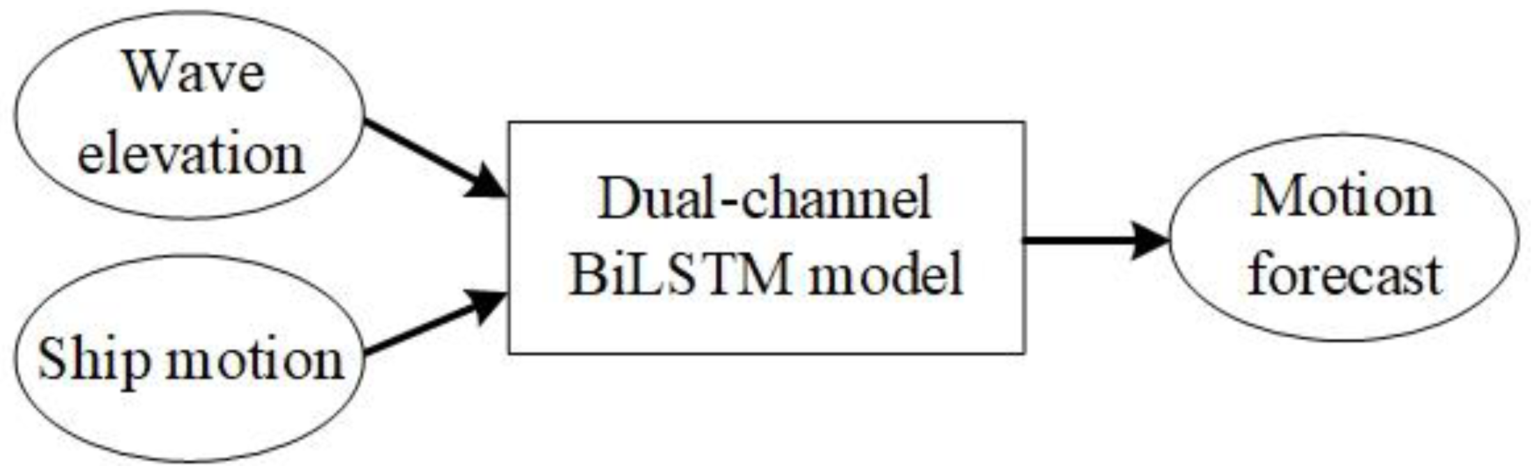
2.2. BiLSTM Network
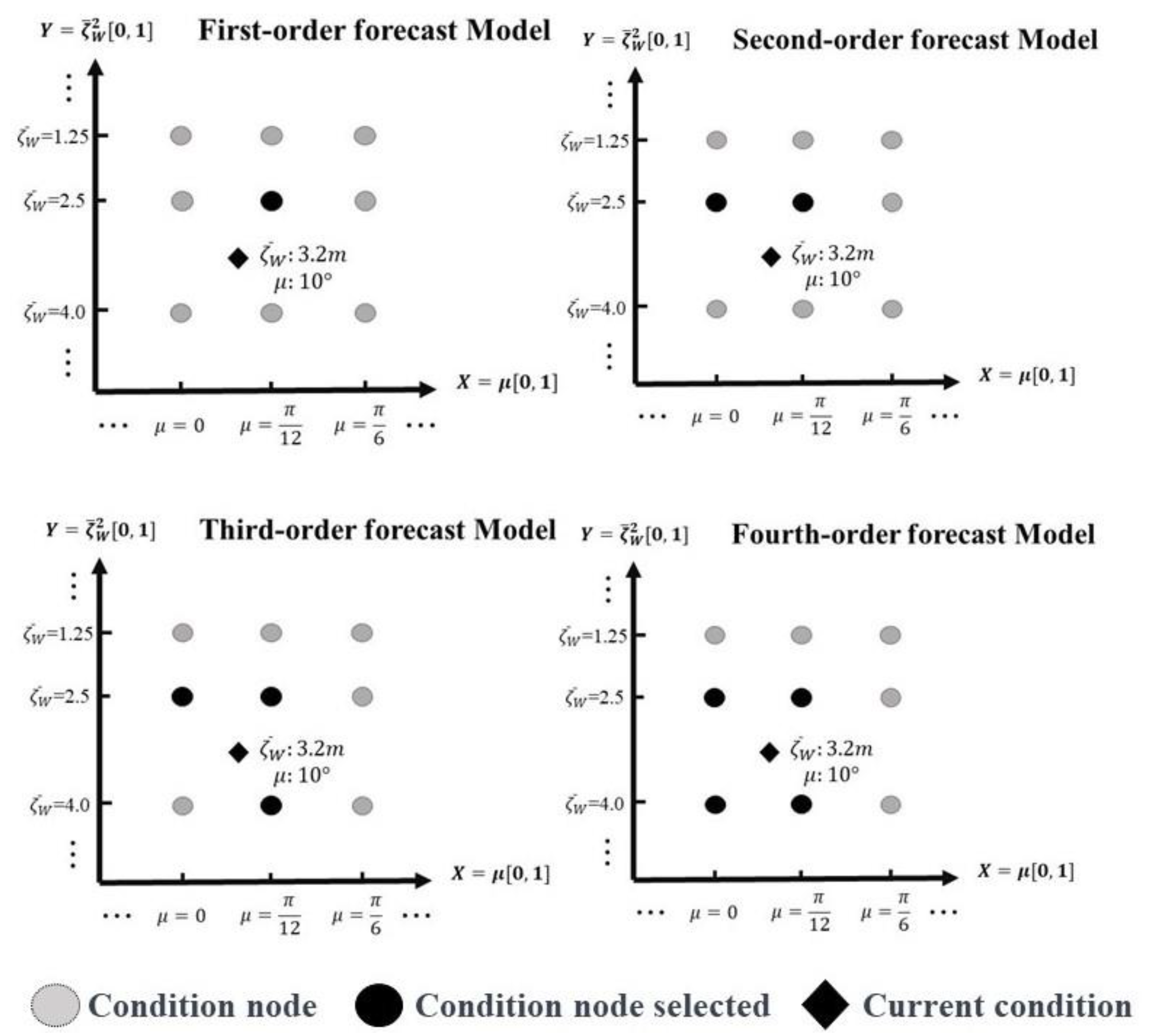
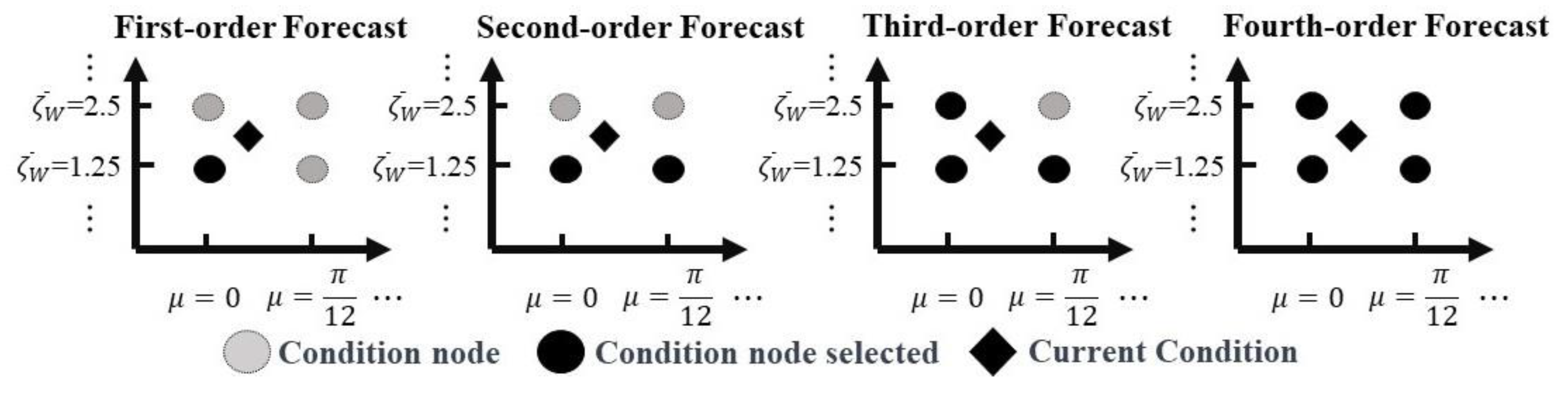
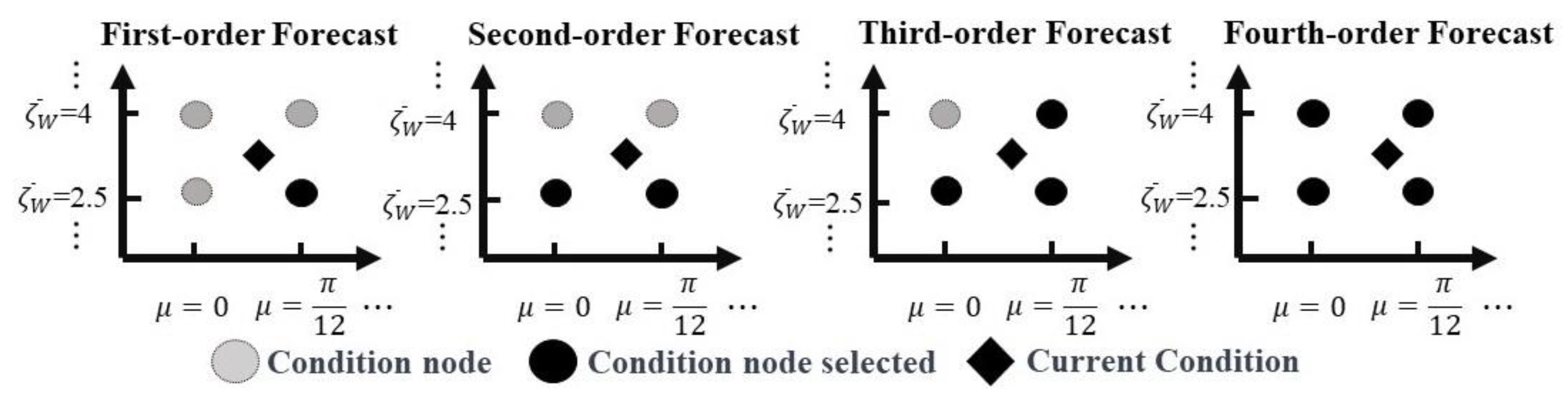
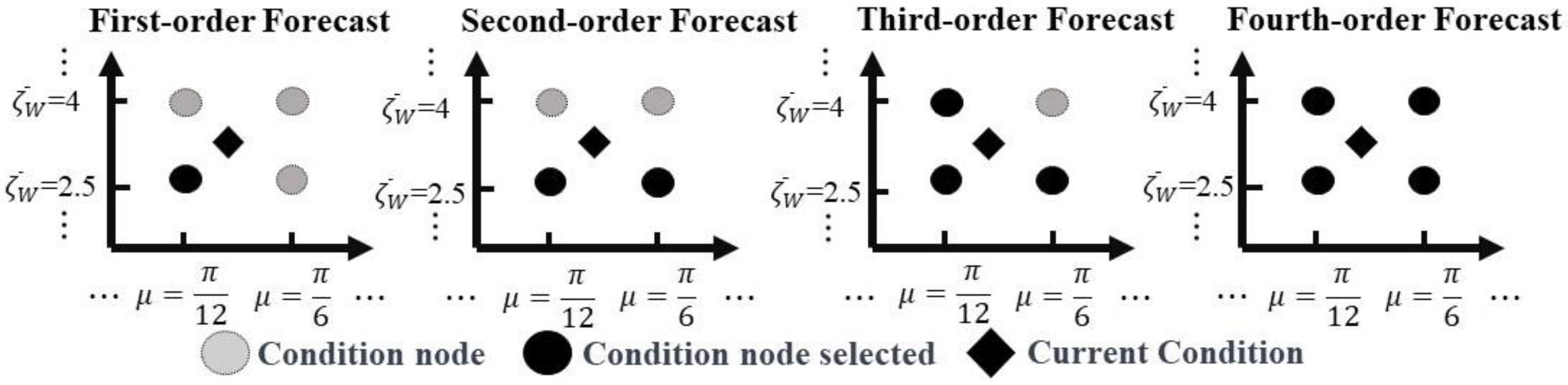
2.3. Dynamic Model Averaging Based on GJO
| Algorithm 1: Condition Node Select | |
| Input: [m, n], where m and n are parameters of ship motion response functions; Condition nodes coordinate sets X, Y | |
| Output: Condition Nodes | |
| 1 | X(m+), Y (n+): Node greater than m or n in that dimension; |
| 2 | X(m−), Y (n−): Node less than m or n in that dimension; |
| 3 | if m X and n Y then |
 | |
| 11 | return Condition Nodes |
3. Experiment
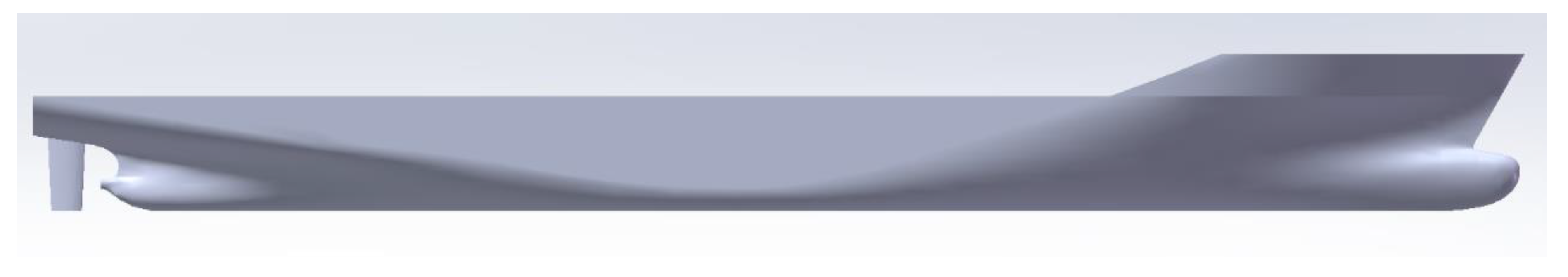
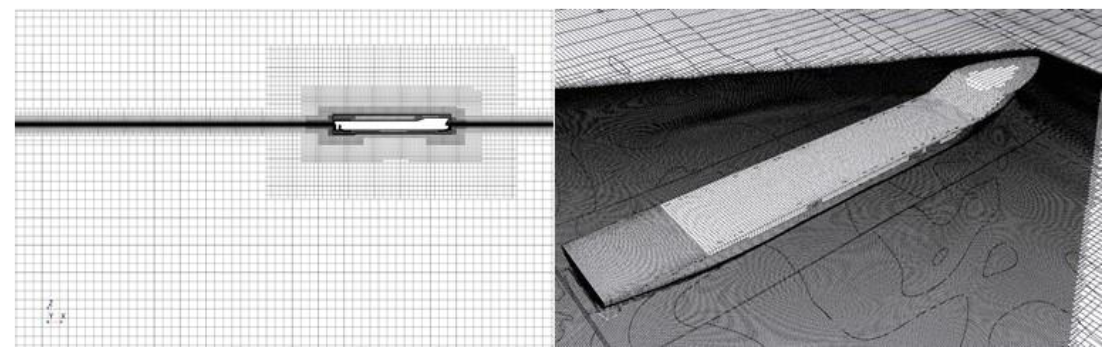
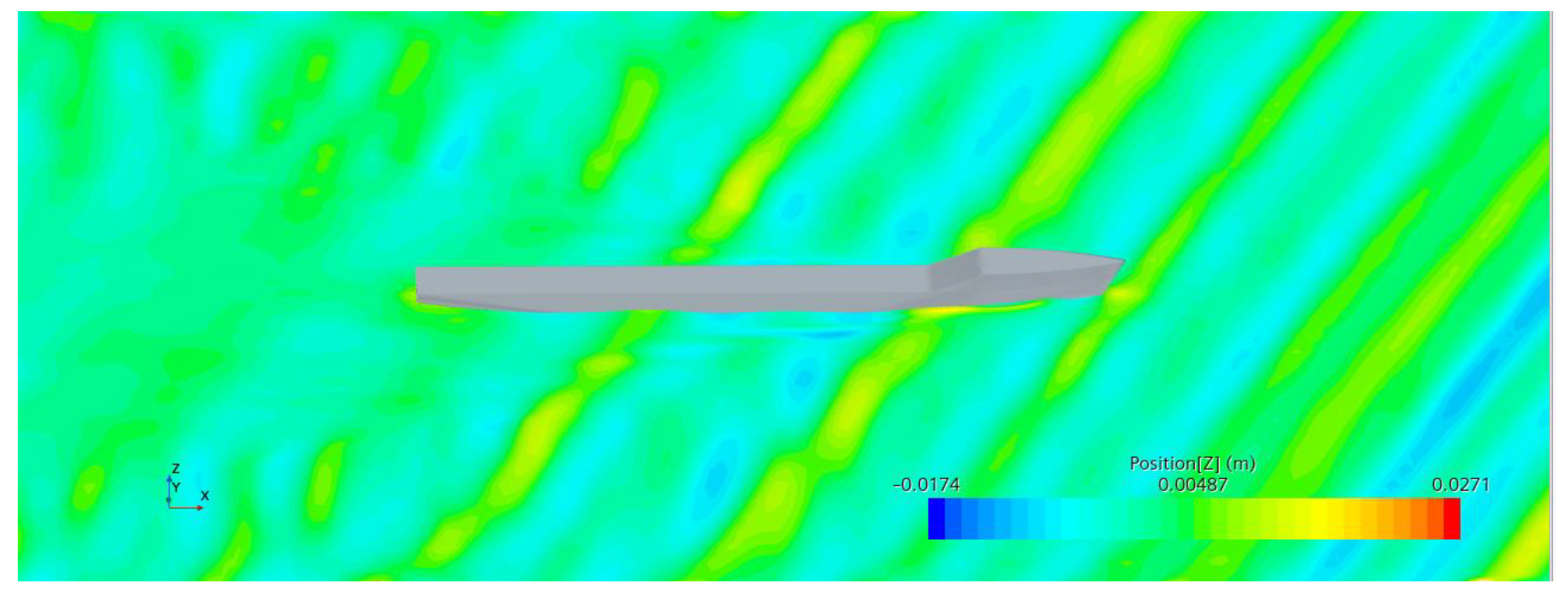
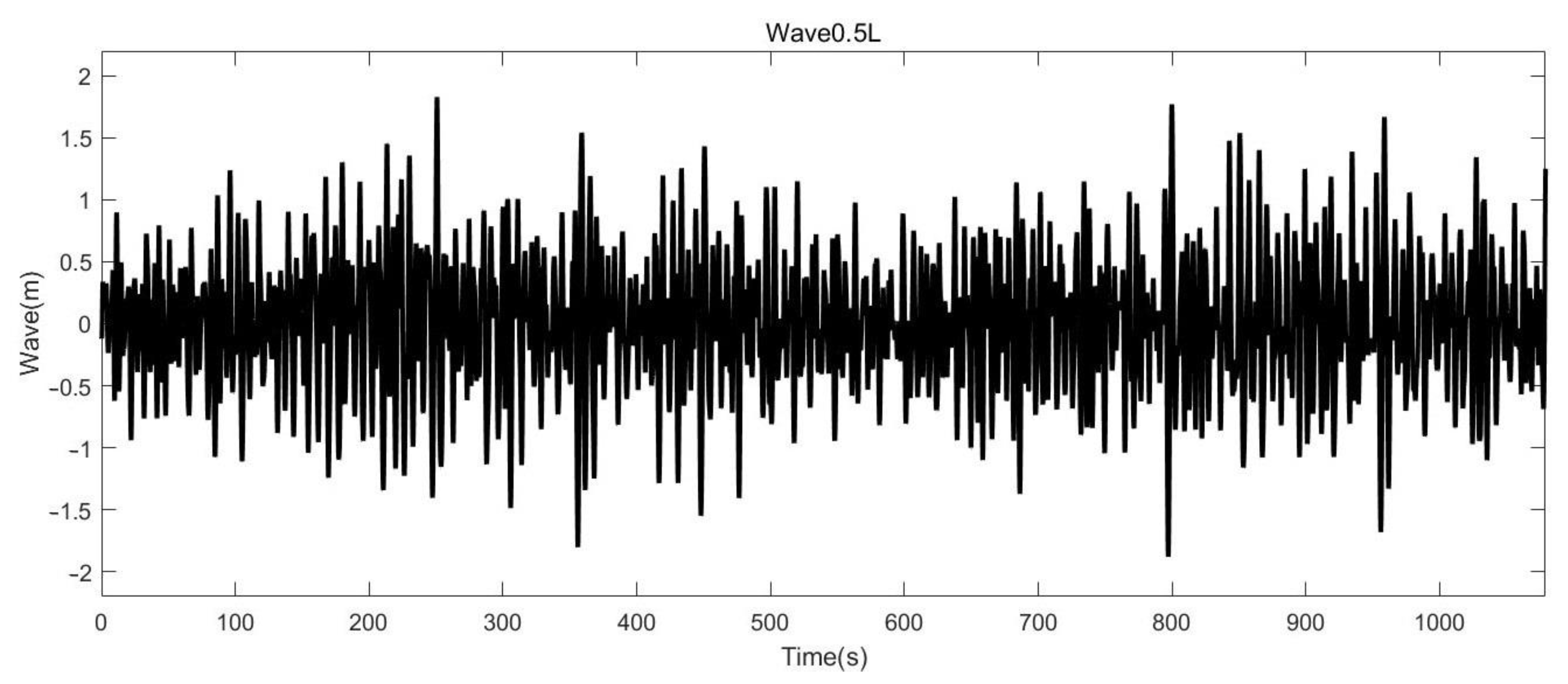
3.1. Numerical Simulation of the KCS Ship
3.2. Pre-Trained Models under Node Conditions
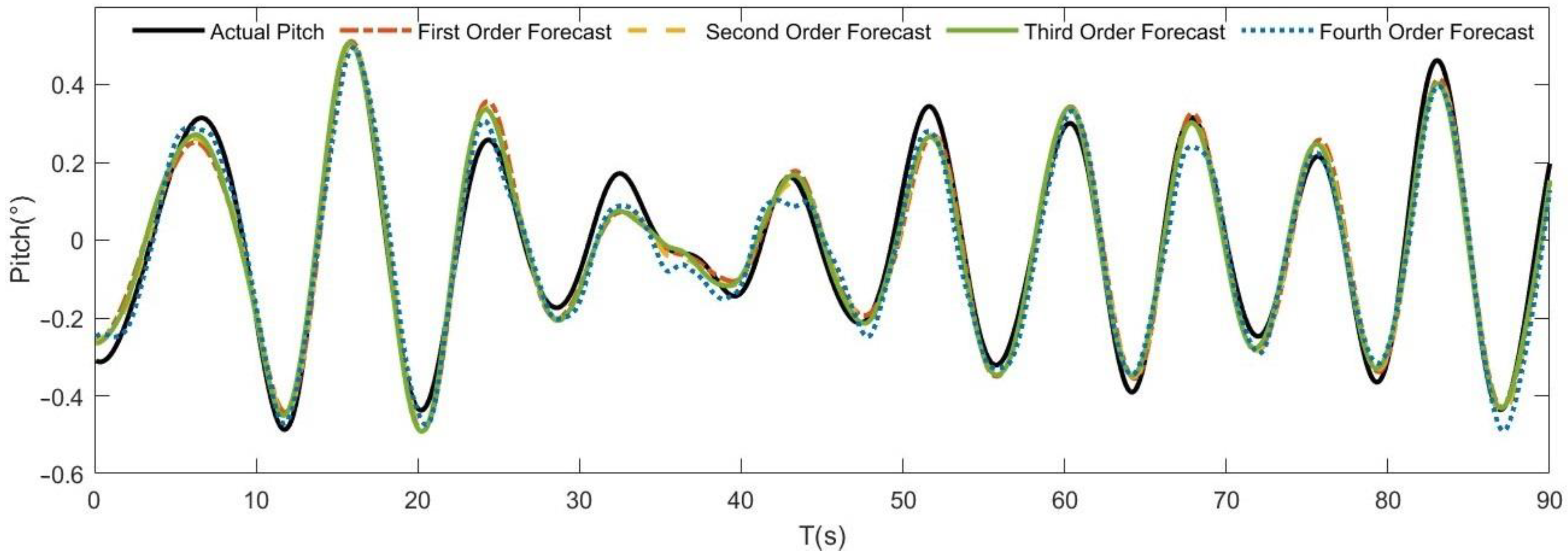
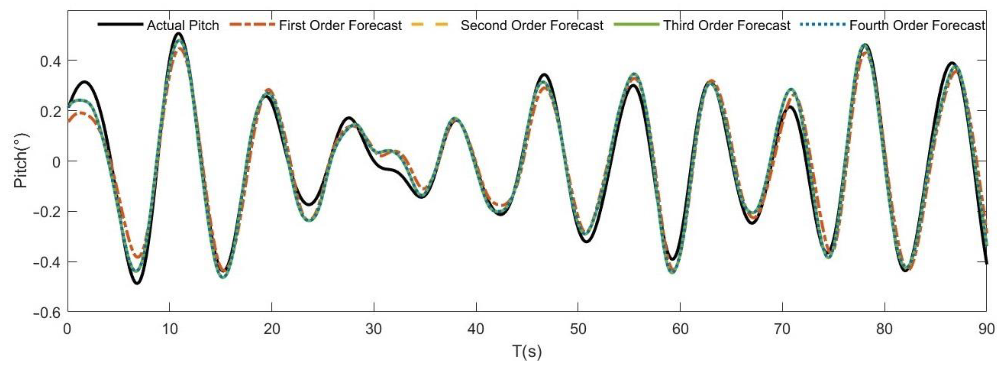
3.3. Motion Forecast under Non-Node Conditions
4. Conclusions
Author Contributions
Funding
Institutional Review Board Statement
Informed Consent Statement
Data Availability Statement
Conflicts of Interest
References
- Kubo, M.; Mizui, S.; Inoue, K. Safety evaluation of ship entering a harbor under severe wave conditions. In Proceedings of the 10th International Offshore and Polar Engineering Conference (ISOPE-2000), Seattle, WA, USA, 28 May–2 June 2000; Grundy, P., Koo, J., Langen, I., Knapp, R., Eds.; ISOPE: Mountain View, CA, USA, 2000; Volume IV, pp. 330–336. [Google Scholar]
- Chu, Y.G.; Li, G.Y.; Hatledal, L.I.; Holmeset, F.T.; Zhang, H.X. Coupling of dynamic reaction forces of a heavy load crane and ship motion responses in waves. Ships Offshore Struct. 2021, 16, 58–67. [Google Scholar] [CrossRef]
- Neupert, J.; Mahl, T.; Haessig, B.; Sawodny, O.; Schneider, K. A heave compensation approach for offshore cranes. In Proceedings of the 2008 American Control Conference, Seattle, WA, USA, 11–13 June 2008; IEEE: Piscataway, NJ, USA, 2008; Volume 1–12, p. 538. [Google Scholar]
- Yang, H.; Pan, Z.; Bai, W. Review of Time Series Prediction Methods. Comput. Sci. 2019, 46, 21–28. [Google Scholar]
- Nie, Z.H.; Lu, Z.F.; Lai, P.; Zhou, J.P.; Yao, F.J. Short-term Prediction of Large Ship Motion Based on Empirical Mode Decomposition and Autoregressive Model. In Proceedings of the 2022 IEEE 6th Advanced Information Technology, Electronic and Automation Control Conference (IAEAC), Beijing, China, 3–5 October 2022; IEEE: Piscataway, NJ, USA, 2022; pp. 933–937. [Google Scholar]
- Peng, X.Y.; Zhang, B.; Rong, L.H. A robust unscented Kalman filter and its application in estimating dynamic positioning ship motion states. J. Mar. Sci. Technol. 2019, 24, 1265–1279. [Google Scholar] [CrossRef]
- Jiang, H.; Duan, S.L.; Huang, L.M.; Han, Y.; Yang, H.; Ma, Q.W. Scale effects in AR model real-time ship motion prediction. Ocean Eng. 2020, 203, 107202. [Google Scholar] [CrossRef]
- Takami, T.; Nielsen, U.D.; Jensen, J.J. Real-time deterministic prediction of wave-induced ship responses based on short-time measurements. Ocean Eng. 2021, 221, 108503. [Google Scholar] [CrossRef]
- Ramadevi, B.; Bingi, K. Chaotic Time Series Forecasting Approaches Using Machine Learning Techniques: A Review. Symmetry 2022, 14, 955. [Google Scholar] [CrossRef]
- D’Agostino, D.; Serani, A.; Stern, F.; Diez, M. Time-series forecasting for ships maneuvering in waves via recurrent-type neural networks. J. Ocean Eng. Mar. Energy 2022, 8, 479–487. [Google Scholar] [CrossRef]
- Silva, K.M.; Maki, K.J. Data-Driven system identification of 6-DoF ship motion in waves with neural networks. Appl. Ocean Res. 2022, 125, 103222. [Google Scholar] [CrossRef]
- Diez, M.; Serani, A.; Campana, E.F.; Stern, F. Time-series forecasting of ships maneuvering in waves via dynamic mode decomposition. J. Ocean Eng. Mar. Energy 2022, 8, 471–478. [Google Scholar] [CrossRef]
- Burkart, N.; Huber, M.F. A Survey on the Explainability of Supervised Machine Learning. J. Artif. Intell. Res. 2021, 70, 245–317. [Google Scholar] [CrossRef]
- Suhermi, N.; Suhartono; Prastyo, D.D.; Ali, B. Roll motion prediction using a hybrid deep learning and ARIMA model. In Proceedings of the 3rd INNS Conference on Big Data and Deep Learning (INNS BDDL), Kota Denpasar, Indonesia, 17–19 April 2018; Ozawa, S., Tan, A.H., Angelov, P.P., Roy, A., Pratama, M., Eds.; Elsevier: Amsterdam, The Netherlands, 2018; Volume 144, pp. 251–258. [Google Scholar]
- Xu, W.Z.; Maki, K.J.; Silva, K.M. A data-driven model for nonlinear marine dynamics. Ocean Eng. 2021, 236, 109469. [Google Scholar] [CrossRef]
- Ye, R.; Dai, Q. A novel transfer learning framework for time series forecasting. Knowl.-Based Syst. 2018, 156, 74–99. [Google Scholar] [CrossRef]
- Du, Y.T.; Wang, J.D.; Feng, W.J.; Pan, S.N.; Qin, T.; Xu, R.J.; Wang, C.J. AdaRNN: Adaptive Learning and Forecasting for Time Series. In Proceedings of the 30th ACM International Conference on Information & Knowledge Management (CIKM), Gold Coast, Australia, 1–5 November 2021; ACM: New York, NY, USA, 2021; pp. 402–411. [Google Scholar]
- Dormann, C.F.; Calabrese, J.M.; Guillera-Arroita, G.; Matechou, E.; Bahn, V.; Barton, K.; Beale, C.M.; Ciuti, S.; Elith, J.; Gerstner, K.; et al. Model averaging in ecology: A review of Bayesian, information-theoretic, and tactical approaches for predictive inference. Ecol. Monogr. 2018, 88, 485–504. [Google Scholar] [CrossRef]
- Darbandsari, P.; Coulibaly, P. Introducing entropy-based Bayesian model averaging for streamflow forecast. J. Hydrol. 2020, 591, 125577. [Google Scholar] [CrossRef]
- Naser, H. Estimating and forecasting the real prices of crude oil: A data rich model using a dynamic model averaging (DMA) approach. Energy Econ. 2016, 56, 75–87. [Google Scholar] [CrossRef]
- Jiang, Y.S.; Jia, M.Q.; Zhang, B.; Deng, L.W. Ship Attitude Prediction Model Based on Cross-Parallel Algorithm Optimized Neural Network. IEEE Access 2022, 10, 77857–77871. [Google Scholar] [CrossRef]
- Wei, Y.Y.; Chen, Z.Z.; Zhao, C.; Tu, Y.H.; Chen, X.; Yang, R. A BiLSTM hybrid model for ship roll multi-step forecasting based on decomposition and hyperparameter optimization. Ocean Eng. 2021, 242, 110138. [Google Scholar] [CrossRef]
- Zhang, G.Y.; Tan, F.; Wu, Y.X. Ship Motion Attitude Prediction Based on an Adaptive Dynamic Particle Swarm Optimization Algorithm and Bidirectional LSTM Neural Network. IEEE Access 2020, 8, 90087–90098. [Google Scholar] [CrossRef]
- Do, K.D.; Jiang, Z.P.; Pan, J. Robust global stabilization of underactuated ships on a linear course: State and output feedback. Int. J. Control 2003, 76, 1–17. [Google Scholar] [CrossRef]
- Seo, M.G.; Kim, Y. Numerical analysis on ship maneuvering coupled with ship motion in waves. Ocean Eng. 2011, 38, 1934–1945. [Google Scholar] [CrossRef]
- Yang, W.; Liang, Y.K.; Leng, J.X.; Li, M. The Autocorrelation Function Obtained from the Pierson-Moskowitz Spectrum. In Proceedings of the Global Oceans 2020: Singapore—U.S. Gulf Coast, Biloxi, MS, USA, 5–30 October 2020; IEEE: Piscataway, NJ, USA, 2020. [Google Scholar]
- Peng, T.; Zhang, C.; Zhou, J.Z.; Nazir, M.S. An integrated framework of Bi-directional long-short term memory (BiLSTM) based on sine cosine algorithm for hourly solar radiation forecasting. Energy 2021, 221, 119887. [Google Scholar] [CrossRef]
- Yu, Y.; Si, X.S.; Hu, C.H.; Zhang, J.X. A Review of Recurrent Neural Networks: LSTM Cells and Network Architectures. Neural Comput. 2019, 31, 1235–1270. [Google Scholar] [CrossRef]
- Raftery, A.E.; Kárny, M.; Ettler, P. Online Prediction Under Model Uncertainty via Dynamic Model Averaging: Application to a Cold Rolling Mill. Technometrics 2010, 52, 52–66. [Google Scholar] [CrossRef]
- Chopra, N.; Ansari, M.M. Golden jackal optimization: A novel nature-inspired optimizer for engineering applications. Expert Syst. Appl. 2022, 198, 116924. [Google Scholar] [CrossRef]
- GB/T 42176-2022; The Grade of Wave Height. General Administration of Quality Supervision. Inspection and Quarantine of the People’s Republic of China: Beijing, China, 2022.
- Shen, Z.; Wan, D.; Carrica, P.M. Dynamic overset grids in OpenFOAM with application to KCS self-propulsion and maneuvering. Ocean Eng. 2015, 108, 287–306. [Google Scholar] [CrossRef]
- Li, Y.; Xiao, L.; Wei, H.; Kou, Y.; Li, X. Comparative Study of Two Neural Network Models for Online Prediction of Wave Run-up on Semi-Submersible. Shipbuild. China 2023, 64, 28–40. [Google Scholar]


| Full Scale | Model | |
|---|---|---|
| Scale | 1 | 80.87 |
| Length between perpendiculars (m) | 230 | 2.844 |
| Design waterline breadth (m) | 32.2 | 0.398 |
| Draught (m) | 10.8 | 0.134 |
| Displacement space(m3) | 52,030 | 0.09836 |
| Level | Sea State | Wave Height |
|---|---|---|
| 0 | Calm-Glassy | 0 m |
| 1 | Calm-Rippled | 0–0.1 m |
| 2 | Smooth-Wavelet | 0.1–0.5 m |
| 3 | Slight | 0.5–1.25 m |
| 4 | Moderate | 1.25–2.5 m |
| 5 | Rough | 2.5–4.0 m |
| 6 | Very Rough | 4.0–6.0 m |
| Wave Approach Angle Sea State | 0° | 15° | 30° | ||||||
|---|---|---|---|---|---|---|---|---|---|
| Pitch | Heave | Pitch | Heave | Pitch | Heave | ||||
| ··· | ··· | ··· | ··· | ··· | ··· | ··· | ··· | ··· | |
| Level-3 () | MAE | 0.0077 | 0.0092 | 0.0081 | 0.0110 | 0.0108 | 0.0139 | ||
| RMSE | 0.0098 | 0.0101 | 0.0105 | 0.0137 | 0.0126 | 0.0187 | |||
| 0.9927 | 0.9901 | 0.9945 | 0.9914 | 0.9901 | 0.9952 | ||||
| Level-4 () | MAE | 0.0191 | 0.0173 | 0.0178 | 0.0267 | 0.0133 | 0.0272 | ||
| RMSE | 0.0234 | 0.0218 | 0.0230 | 0.0318 | 0.0168 | 0.0323 | |||
| 0.9923 | 0.9870 | 0.9964 | 0.9933 | 0.9979 | 0.9963 | ||||
| Level-5 () | MAE | 0.0314 | 0.0352 | 0.0443 | 0.0609 | 0.0343 | 0.0527 | ||
| RMSE | 0.0411 | 0.0435 | 0.0550 | 0.0755 | 0.0428 | 0.0647 | |||
| 0.9975 | 0.9937 | 0.9985 | 0.9957 | 0.9981 | 0.9916 | ||||
| ··· | ··· | ··· | ··· | ··· | ··· | ··· | ··· | ||
| Wave Approach Angle Sea State | 0° | 15° | 30° | ||||||
|---|---|---|---|---|---|---|---|---|---|
| Pitch | Heave | Pitch | Heave | Pitch | Heave | ||||
| ··· | ··· | ··· | ··· | ··· | ··· | ··· | ··· | ··· | |
| Level-3 () | MAE | 0.0093 | 0.0101 | 0.0075 | 0.0139 | 0.0191 | 0.0176 | ||
| RMSE | 0.0178 | 0.0186 | 0.0165 | 0.0208 | 0.0232 | 0.0254 | |||
| 0.9891 | 0.9922 | 0.9907 | 0.9854 | 0.9927 | 0.9863 | ||||
| Level-4 () | MAE | 0.0179 | 0.0231 | 0.0213 | 0.0196 | 0.0198 | 0.0240 | ||
| RMSE | 0.0214 | 0.0282 | 0.0262 | 0.0260 | 0.0238 | 0.0305 | |||
| 0.9945 | 0.9783 | 0.9960 | 0.9930 | 0.9978 | 0.9924 | ||||
| Level-5 () | MAE | 0.0390 | 0.0372 | 0.0529 | 0.0592 | 0.0618 | 0.0871 | ||
| RMSE | 0.0218 | 0.0476 | 0.0649 | 0.0718 | 0.0777 | 0.1102 | |||
| 0.9960 | 0.9927 | 0.9984 | 0.9959 | 0.9917 | 0.9762 | ||||
| ··· | ··· | ··· | ··· | ··· | ··· | ··· | ··· | ||
| Wave Approach Angle Sea State | 0° | 15° | 30° | ||||||
|---|---|---|---|---|---|---|---|---|---|
| Pitch | Heave | Pitch | Heave | Pitch | Heave | ||||
| ··· | ··· | ··· | ··· | ··· | ··· | ··· | ··· | ··· | |
| Level-3 () | MAE | 0.0243 | 0.0324 | 0.0237 | 0.0303 | 0.0294 | 0.0408 | ||
| RMSE | 0.0377 | 0.0433 | 0.0482 | 0.0502 | 0.0412 | 0.0597 | |||
| 0.9698 | 0.9742 | 0.9707 | 0.9654 | 0.9662 | 0.9595 | ||||
| Level-4 () | MAE | 0.0359 | 0.0353 | 0.0549 | 0.0469 | 0.0577 | 0.0515 | ||
| RMSE | 0.0460 | 0.0431 | 0.0676 | 0.0573 | 0.0698 | 0.0622 | |||
| 0.9743 | 0.9513 | 0.9732 | 0.9671 | 0.9706 | 0.9615 | ||||
| Level-5 () | MAE | 0.1455 | 0.1509 | 0.1571 | 0.2017 | 0.1614 | 0.1765 | ||
| RMSE | 0.1805 | 0.2062 | 0.2075 | 0.2908 | 0.1988 | 0.2185 | |||
| 0.9785 | 0.9655 | 0.9814 | 0.9423 | 0.9469 | 0.9398 | ||||
| ··· | ··· | ··· | ··· | ··· | ··· | ··· | ··· | ||
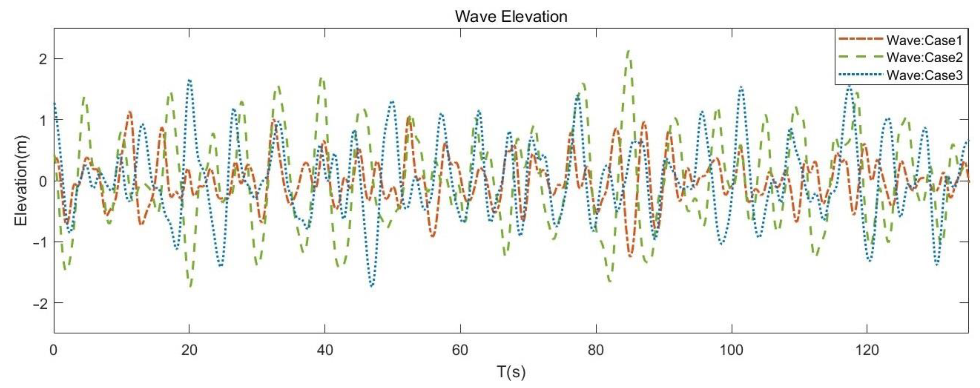
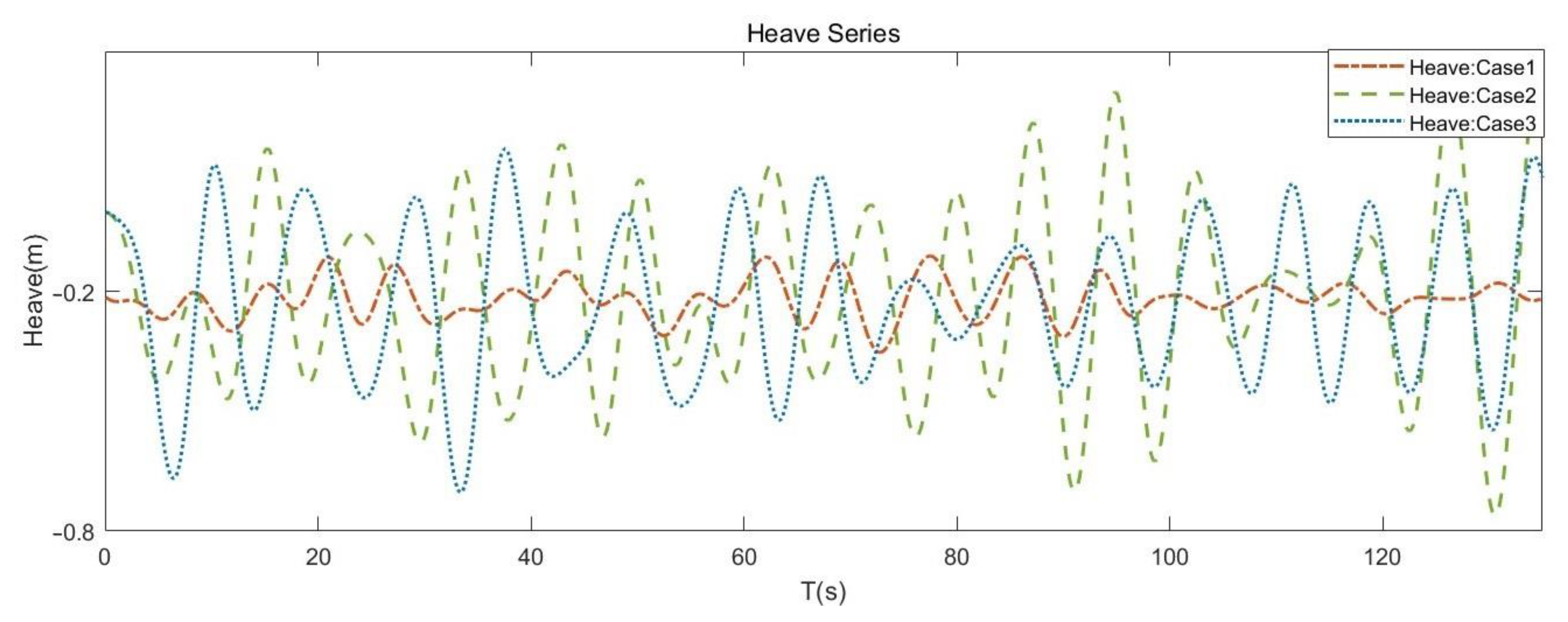
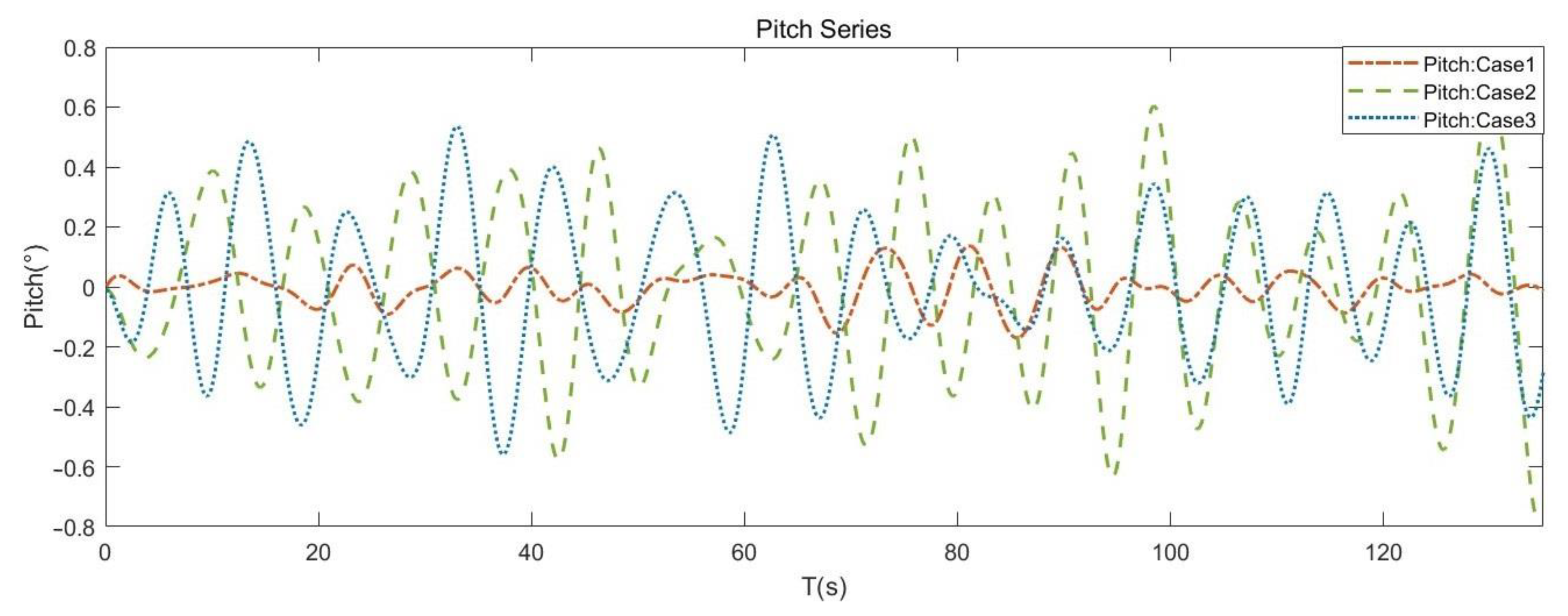
| Case 1 | Case 2 | Case 3 | |
|---|---|---|---|
| (Full Scale, m) | 1.617 | 3.235 | 3.235 |
| (Model, m) | 0.020 | 0.040 | 0.040 |
| (°) | 5° | 10° | 20° |
| First-Order | First-Order | First-Order | First-Order | |
|---|---|---|---|---|
| Params (K) | 298.6 | 597.2 | 895.8 | 1194.5 |
| Case 1 | Case 2 | Case 3 | |||||
|---|---|---|---|---|---|---|---|
| Pitch | Heave | Pitch | Heave | Pitch | Heave | ||
| 5 s Forecast | MAE | 0.0118 | 0.0109 | 0.0462 | 0.0495 | 0.0360 | 0.0267 |
| RMSE | 0.0291 | 0.0188 | 0.0583 | 0.0627 | 0.0437 | 0.0523 | |
| 0.9594 | 0.9531 | 0.9801 | 0.9736 | 0.9821 | 0.9750 | ||
| 10 s Forecast | MAE | 0.0207 | 0.0282 | 0.0542 | 0.0493 | 0.0402 | 0.0415 |
| RMSE | 0.0314 | 0.0340 | 0.0643 | 0.0644 | 0.0478 | 0.0548 | |
| 0.9415 | 0.9495 | 0.9764 | 0.9698 | 0.9807 | 0.9522 | ||
| 15 s Forecast | MAE | 0.0387 | 0.0305 | 0.0935 | 0.0753 | 0.0701 | 0.0618 |
| RMSE | 0.0442 | 0.0479 | 0.1163 | 0.0959 | 0.0892 | 0.0784 | |
| 0.9139 | 0.9277 | 0.9410 | 0.9105 | 0.9384 | 0.9132 | ||
| Case 1 | Case 2 | Case 3 | |||||
|---|---|---|---|---|---|---|---|
| Pitch | Heave | Pitch | Heave | Pitch | Heave | ||
| 5 s Forecast | MAE | 0.0102 | 0.0103 | 0.0443 | 0.0455 | 0.0349 | 0.0226 |
| RMSE | 0.0265 | 0.0164 | 0.0563 | 0.0572 | 0.0410 | 0.0338 | |
| 0.9643 | 0.9562 | 0.9814 | 0.9749 | 0.9847 | 0.9826 | ||
| 10 s Forecast | MAE | 0.0193 | 0.0257 | 0.0465 | 0.0468 | 0.0302 | 0.0397 |
| RMSE | 0.0302 | 0.0339 | 0.0590 | 0.0600 | 0.0368 | 0.0540 | |
| 0.9430 | 0.9546 | 0.9790 | 0.9698 | 0.9879 | 0.9545 | ||
| 15 s Forecast | MAE | 0.0346 | 0.0287 | 0.0628 | 0.0654 | 0.0677 | 0.0592 |
| RMSE | 0.0412 | 0.0455 | 0.0788 | 0.0838 | 0.0833 | 0.0745 | |
| 0.9315 | 0.9410 | 0.9607 | 0.9233 | 0.9534 | 0.9237 | ||
| Case 1 | Case 2 | Case 3 | |||||
|---|---|---|---|---|---|---|---|
| Pitch | Heave | Pitch | Heave | Pitch | Heave | ||
| 5 s Forecast | MAE | 0.0101 | 0.0103 | 0.0442 | 0.0455 | 0.0319 | 0.0220 |
| RMSE | 0.0265 | 0.0164 | 0.0564 | 0.0572 | 0.0391 | 0.0328 | |
| 0.9644 | 0.9562 | 0.9814 | 0.9741 | 0.9859 | 0.9833 | ||
| 10 s Forecast | MAE | 0.0193 | 0.0258 | 0.0465 | 0.0467 | 0.0302 | 0.0390 |
| RMSE | 0.0301 | 0.0339 | 0.0590 | 0.0598 | 0.0368 | 0.0540 | |
| 0.9430 | 0.9546 | 0.9790 | 0.9698 | 0.9879 | 0.9546 | ||
| 15 s Forecast | MAE | 0.0344 | 0.0295 | 0.0627 | 0.0643 | 0.0677 | 0.0592 |
| RMSE | 0.0412 | 0.0451 | 0.0787 | 0.0832 | 0.0833 | 0.0745 | |
| 0.9317 | 0.9413 | 0.9607 | 0.9254 | 0.9534 | 0.9237 | ||
| Case 1 | Case 2 | Case 3 | |||||
|---|---|---|---|---|---|---|---|
| Pitch | Heave | Pitch | Heave | Pitch | Heave | ||
| 5 s Forecast | MAE | 0.0102 | 0.0103 | 0.0442 | 0.0455 | 0.0319 | 0.0220 |
| RMSE | 0.0265 | 0.0166 | 0.0563 | 0.0572 | 0.0391 | 0.0328 | |
| 0.9643 | 0.9562 | 0.9814 | 0.9741 | 0.9858 | 0.9833 | ||
| 10 s Forecast | MAE | 0.0193 | 0.0257 | 0.0465 | 0.0467 | 0.0301 | 0.0397 |
| RMSE | 0.0302 | 0.0339 | 0.0590 | 0.0598 | 0.0368 | 0.0539 | |
| 0.9430 | 0.9545 | 0.9790 | 0.9698 | 0.9879 | 0.9545 | ||
| 15 s Forecast | MAE | 0.0344 | 0.0295 | 0.0628 | 0.0643 | 0.0679 | 0.0592 |
| RMSE | 0.0412 | 0.0455 | 0.0788 | 0.0832 | 0.0836 | 0.0745 | |
| 0.9315 | 0.9410 | 0.9607 | 0.9254 | 0.9531 | 0. 9237 | ||
Disclaimer/Publisher’s Note: The statements, opinions and data contained in all publications are solely those of the individual author(s) and contributor(s) and not of MDPI and/or the editor(s). MDPI and/or the editor(s) disclaim responsibility for any injury to people or property resulting from any ideas, methods, instructions or products referred to in the content. |
© 2024 by the authors. Licensee MDPI, Basel, Switzerland. This article is an open access article distributed under the terms and conditions of the Creative Commons Attribution (CC BY) license (https://creativecommons.org/licenses/by/4.0/).
Share and Cite
Jiang, Z.; Ma, Y.; Li, W. A Data-Driven Method for Ship Motion Forecast. J. Mar. Sci. Eng. 2024, 12, 291. https://doi.org/10.3390/jmse12020291
Jiang Z, Ma Y, Li W. A Data-Driven Method for Ship Motion Forecast. Journal of Marine Science and Engineering. 2024; 12(2):291. https://doi.org/10.3390/jmse12020291
Chicago/Turabian StyleJiang, Zhiqiang, Yongyan Ma, and Weijia Li. 2024. "A Data-Driven Method for Ship Motion Forecast" Journal of Marine Science and Engineering 12, no. 2: 291. https://doi.org/10.3390/jmse12020291