Article

Fluid Structure Interaction Using Modal Superposition and Lagrangian CFD

1
Faculty of Electrical Engineering, Mechanical Engineering and Naval Architecture, University of Split, Ruđera Boškovića 32, 21000 Split, Croatia
2
Engineering Software Steyr, Berggasse 35, 4400 Steyr, Austria
3
Faculty of Mechanical Engineering and Naval Architecture, University of Zagreb, Ivana Lučića 5, 10000 Zagreb, Croatia
*
Author to whom correspondence should be addressed.
J. Mar. Sci. Eng. 2024, 12(2), 318; https://doi.org/10.3390/jmse12020318
Submission received: 6 January 2024 / Revised: 6 February 2024 / Accepted: 8 February 2024 / Published: 12 February 2024
(This article belongs to the Special Issue CFD Applications in Ship and Offshore Hydrodynamics)

Abstract

:
This study investigates the impact of fluid loads on the elastic deformation and dynamic response of linear structures. A weakly coupled modal solver is presented, which involves the solution of a dynamic equation of motion with external loads. The mode superposition method is used to find the dynamic response, utilizing predetermined mode shapes and natural frequencies associated with the structure. These essential parameters are pre-calculated and provided as input for the simulation. Integration of the weakly coupled modal solver is accomplished with the Lagrangian Differencing Dynamics (LDD) method. This method can directly use surface mesh as boundary conditions, so it is much more convenient than other meshless CFD methods. It employs Lagrangian finite differences, utilizing a strong formulation of the Navier–Stokes equations to model an incompressible free-surface flow. The elastic deformation of the structure, induced by fluid forces obtained from the flow solver, is computed within the modal coupling algorithm through direct numerical integration. Subsequently, this deformation is introduced into the flow solver to account for changes in geometry, resulting in updated flow pressure and velocity fields. The flow particles and vertices of the structure are advected in Lagrangian coordinates, resulting in Lagrangian–Lagrangian coupling in spaces with weak or explicit coupling in time. The two-way coupling between fluid and structure is successfully validated through various FSI benchmark cases. The efficiency of the LDD method is highlighted as it operates directly on surface meshes, streamlining the simulation setup. Direct coupling of structural deformation eliminates the conventional step of mapping fluid results onto the structural mesh and vice versa.

1. Introduction

The Fluid–Structure Interaction (FSI) is the most prevalent physical phenomenon in various engineering applications. Some of the applications, such as the interaction between waves and vegetation in coastal wetlands and wave–ice interactions in the Arctic environment [1], are crucial in mitigating coastal flooding [2]. FSI plays a pivotal role in the refinement of structural designs for optimal performance under fluid loads, ensuring both efficiency and reliability [3], e.g., the construction of offshore installations and the design of windmills and ships. Identifying FSI-related issues early allows cost-effective design changes, reducing the need for any modifications during manufacturing or operation [4]. Similarly, FSI affects the hydrodynamic performance of propellers, e.g., [5,6]. The damping represents energy dissipation within vibration cycles and emerges as a key factor in resonance phenomena, impacting harmonic vibration amplitudes and the count of noteworthy vibrations in time-dependent scenarios. In most cases, the role of damping can be negligible in slightly damped vibrations. However, in the natural frequencies, their influence becomes pronounced, especially in near-resonant conditions, where excitation is balanced solely through damping. Damping in the structure is generally low, except when near resonance and the vibration cycle maintains a substantial level of independence [7].
However, simulating FSI effectively is complex, requiring certain assumptions in both structural and fluid simulations. In most of the Computational Fluid Dynamics (CFD) simulations, the consideration of elastic deformation at the boundaries is ignored [8]. Similarly, in most of the structural simulations, a constant pressure is considered at the interior and exterior boundaries. Paik et al. [9] presented methods for coupling the CFD solver with rigid and elastic models of a ship hull to compute structural loads. One-way and two-way coupling approaches were used when considering the ship as elastic. In one-way coupling, forces from CFD were used for structural loads analysis, but deformations were not feedback to CFD. In two-way coupling, hull deformations influenced the CFD solution. A URANS/DES overset solver with the modal superposition method is used for the analysis. The gluing method was applied to transfer forces and deformations between non-matching CFD and structural grids [9].
Different varieties of approaches have been formulated to tackle the intricacies of one-way and two-way coupling of the FSI. A prominent approach involves fully coupled (monolithic) methods that integrate structural and flow calculations in a single solver [10,11]. Conventional CFD solvers predominantly use an Eulerian-based approach. However, such coupling of structural formulations, which mostly use Lagrangian-based approaches, leads to a stiffer computation for the structural component compared to the fluid component. Moreover, employing a unified scheme for extensive scenarios becomes computationally intensive [12].
Grid-based partitioned methods offer a more feasible alternative to monolithic methods by tackling both the flow and structural formulation on two different meshes using distinct solvers [13]. These methods necessitate the establishment of a communication protocol at the interface between grids to appropriately transfer fluid loads to the structural mesh and, conversely, to map the deformation onto the fluid mesh. In mesh-based solvers, effective adjustment of the fluid mesh boundaries requires precise manipulation of adjacent mesh nodes to prevent mesh entanglement or deformation [14,15]. Recent advances have demonstrated the successful application of partitioned methods, such as coupling thin-walled girder theory with potential flow theory [16,17] and linking modal structure solvers with RANS-VOF solvers, Boundary-Integral Equation Methods [18]. Solid4Foam with the finite volume library is provided by OpenFOAM [19,20].
The meshless-based partitioned method offers several advantages, especially in scenarios that involve free surfaces, violent flow, complex models, and large deformations [21]. In this approach, the need for re-meshing of the model after deformation is effectively avoided. FSI is achieved by coupling the Smooth Particle Hydrodynamics (SPH) with different structural solvers such as the Finite Element Method (FEM) [22,23,24] and Discrete Element Method (DEM) [25,26,27] to compute the structural deformation. However, transferring the information is not easy, as it is necessary to resolve the interfacial energy balance [28]. Solving the structural deformation is computationally expensive but less so than the monolithic method.
In recent days, the Mode Superposition method has been used to solve structural deformation, and it is the most robust, fast, and computationally inexpensive method. Debrabandere et al. (2012) presented a new reduced-order modeling approach for FSI simulations. The method uses modal analysis to represent structural dynamics, solving the modal equations within the computational fluid dynamics solver using a complementary function and a particular integral method. Results for simple test cases compare well with full-order models and experiments. FSI predictions for realistic turbomachinery configurations demonstrate the potential of the method for efficient aeroelastic analysis of flexible structures [29]. Sun et al. (2019) presented the Moving Particle Semi-implicit (MPS) with the mode superposition method to simulate violent hydroelastic issues [30]. Corrado et al. (2020) validated the two-way coupling between CFD and FEM solvers and a more efficient modal superposition approach with the help of the HIRENASD test case [31]. Modal superposition is a useful technique for evaluating structures that are subjected to dynamic loads due to its computational efficiency and simplicity. However, when dealing with large structural deformations, the accuracy of this method tends to decrease. This is because modal superposition assumes linear behavior and uncoupled modes, which may not hold true in scenarios involving significant nonlinearity or mode coupling. Despite these limitations, modal superposition remains a widely used and valuable tool, especially when applied within its valid range [29,30,31]. Weak coupling in FSI offers simplicity and ease of implementation, making it suitable for scenarios with transient events. However, its limitations include stability issues necessitating small time steps, which can lead to computational inefficiency, and potential accuracy trade-offs compared to implicit methods, especially in large-scale simulations where the fluid and structural solvers use time steps of different magnitudes [32]. The convenience of using modes superposition is that the structural solver adds insignificant computational cost [17,29] and therefore, can adjust to the flow solver requirements.
The aim of this study is to develop a model for Fluid–Structure Interaction (FSI) by combining the Mode Superposition method and the Lagrangian Differencing Dynamics (LDD) method in two-way partitioned weak coupling or explicit coupling. In terms of computational efficiency, the LDD method is advantageous compared to most popular meshless approaches, such as Smoothed Particle Hydrodynamics (SPH), Moving Particle Semi-implicit (MPS), finite point set method, and finite point method [33,34,35]. The LDD method achieves large time steps with lower computational costs while maintaining second-order accuracy. It is well-suited for complex transient problems since it has the advantage of directly working on the meshes [8,16,17,36]. Using the mode superposition method with LDD, structural deformation is calculated for the fluid load using precalculated mode shapes and natural frequencies from the modal analysis. This approach leads to stable, robust, and computationally efficient FSI simulations. The method enables fluid-induced structural deformation to be weakly coupled into the flow solver. The deformation is obtained by using direct integration. The flow particles and vertices of the structure are advected in Lagrangian coordinates. This results in Lagrangian–Lagrangian coupling in space, while there is weak or explicit coupling in time. This ensures a more accurate representation of the interaction between fluid and structure in ship and offshore hydrodynamics. The efficiency of the LDD and Mode Superposition methods, operating directly on surface meshes, may lead to practical and effective ship and offshore hydrodynamic simulations.
This paper discusses fluid–structure interaction (FSI) modeling using the two-way weak coupling approach. Specifically, this paper details the governing equation of the LDD method and the mode superposition technique in Section 2. The methodology of implementing two-way coupling of FSI is then explained in Section 3. In Section 4, various benchmark cases are presented that are then validated and verified with modal coupling results. Finally, concluding remarks and a summary of the findings are given in Section 5.

2. Governing Equation

2.1. Incompressible Fluid Flow

An incompressible fluid flow solver known as LDD is employed, which utilizes a generalized finite difference method with a meshless approach. It uses a robust and implicit formulation of the Navier–Stokes equations to simulate incompressible free-surface fluids. This solver is utilized to address initial boundary value problems, achieving second-order accuracy in its solution. It has been successfully validated in various scenarios, including lid-driven cavity, dam break, sloshing, water entry, etc. [8,36,37]. The continuity and momentum equations are provided below:
D u D t = 1 ρ p + ν 2 u + g , x Ω ,
. u = 0 x Ω Γ w Γ f s ,
u = U x Γ w ,
u ( t = 0 ) = u 0 x Ω
In this context, D D t signifies the time rate of change of a property, u stands for the velocity vector, ρ represents the fluid density, p denotes the dynamic pressure, υ symbolizes the kinematic viscosity, g represents gravity, U corresponds to the wall velocity, and u 0 denotes the initial velocity vector.
The pressure and velocity equations are solved in a decoupled manner. The pressure Poisson and the pressure gradient equations are presented as follows:
2 p = ρ · D u / D t x Ω , n · p = ρ n · [ D u D t + g + ν 2 u ] x Γ w p = p a t m , x Γ f s
where n represents the normal vector at walls, p a t m represents atmospheric pressure, and g is the gravity constant. Additional information can be found in [8,36,37,38]. The gradient and Laplacian operators from Basic et al. [38] are utilized to discretize the equations mentioned above. To calculate the value of a general function, denoted by f, at a specific node i, the neighbouring nodes represented by j within a compact radius of h are taken into account. The differential operators, which are based on [38], are defined as:
f i = B i j I W i j r i j f j f i
2 f i = 2 d j ϵ N W i j f j f i ( 1 r i j . B i o i ) j ϵ N W i j ( 1 r i j . B i o i ) r i j 2
where, r i j = r j r i denotes the vector between locations of points i and j, while r i and r j denote the positions of points i and j in the fluid domain. The distance between these points is a scalar defined as r i j = r i j . The weighting function W i j = W ( r i j , h ) depends on the distance r i j , defined within some radius of the compact sphere, h. Here, f i and f j represent the function values at locations r i and r j , respectively. The symmetric renormalization tensor B i , and the offset vector o i are, respectively, defined as:
B i = j I W i j r i j r i j 1
o i = j I W i j r i j
The solution of a time step in the LDD method initiates with the Lagrangian advection of points, i.e., the points are moved in space according to their velocities. The streamlines compressibility issues that arise during Lagrangian advection are resolved using the Particle-Based Dynamics (PBD) technique, which iteratively rearranges the locations of points by enforcing a uniform distances between neighbor points [8]. Following this, the pressure Poisson Equation (PPE) defined above is discretized by using the discrete operators, that are defined above and analyzed in [38]. In this study, the PPE is solved using the preconditioned BiCGSTAB linear solver, as explained in [8]. After solving the PPE, the velocity equation arising from the momentum Equation (1) is explicitly determined for each time step.

2.2. Mode Superposition

The method of modal superposition is employed to analyze the dynamic behavior of structures. It is estimated through the superposition of a limited number of modal frequencies obtained from the modal analysis. Modal analysis comes into play to determine the vibration characteristics, primarily the modes of operation and the natural frequencies of a mechanical system or component. Natural frequency, or eigenfrequency, denotes the frequency at which a system naturally oscillates without any external driving force. On the other hand, mode shapes, also referred to as eigenvectors, depict the inherent behavior of the component at its natural frequency. Both these parameters hold significance in the structural design process, especially for scenarios involving dynamic loads. This approach is particularly effective in minimizing computational efforts when evaluating the dynamic response of linear structures [16,39]. This technique proves advantageous especially when dealing with limited known loading frequencies. However, it is less applicable to the issues that encompass exceedingly high frequencies [29,31].
The dynamic equation for a structure can be represented in matrix form as follows:
M u ¨ + C u ˙ + Ku = f t
In this equation, M denotes the mass-normalized matrix, C represents the damping matrix, and K stands for the stiffness matrix. The column vector u corresponds to the degree of freedom, while f ( t ) represents the applied forces over time. These matrices are obtained through the discretization of the physical domain, resulting in an NxN matrix where N signifies the degrees of freedom of the structural model. Mass normalization is convenient in the modal superposition, as it ensures that the modal mass is consistent across all modes, simplifying the modal participation factors and making them directly interpretable as a percentage of total mass.
The foundation of modal superposition is rooted in modal analysis, yielding essential outputs such as eigenfrequencies and their corresponding mode shapes. The eigenfrequencies are computed via the undamped dynamic equation, treated as an eigenvalue problem:
( ω 2 M + K ) Φ = 0 , m m m m m m Φ 0
In this context, the symbol Φ refers to the modal matrix, which contains a vector of the mode shape corresponding to every natural frequency of the structure with n-DOF, Φ = Φ 1 , Φ 2 , . . . , Φ n . Usually, the Finite Element Method (FEM) is used to model a structure, and discretize and solve Equation (11). Multiple numerical methods exist for determining natural frequencies and mode shapes, as no single method is universally optimal for all problems. The techniques for extracting eigenvalues fall under the category of transformation methods and/or tracking methods. The eigenvalue equation is initially converted into a specific format in the transformation method, facilitating the extraction of eigenvalues. The tracking method involves extracting the eigenvalues individually through an iterative procedure. In this study, the Lanczos method was used, which combines characteristics of the tracking and transformation methods. Mass normalization involves scaling the mode shapes such that the square of the mode shape integrated over the structure equals one. This ensures that each mode shape has a unit mass and simplifies the subsequent modal superposition calculations.
After the vibration modes and frequencies are extracted, their combination may be used to simulate complex vibration of the structure. The superposition involves expressing the displacement response as a linear combination of modal contributions. The overall displacement ( u ( t ) ) of the structural system for a time step can be represented as a combination of mode shapes:
u ( t ) = i = 1 n Φ y i ( t )
where y ( t ) is the vector of modal coordinates (or generalized displacement). While one can extract many vibration modes from a FEM model, in engineering practice, usually only first few modes are relevant for analysis. By applying the generalized displacement and the mass normalized modal vector Φ (i.e., substituting Equation (12) into Equation (10)), the following is obtained:
Φ T M Φ y ¨ ( t ) + Φ T C Φ y ˙ ( t ) + Φ T K Φ y ( t ) = Φ T f ( t )
To decouple the equation of motion for a Multi-Degree-of-Freedom (MDOF) system into n equations of motion for Single Degree of Freedom (SDOF) systems, it is necessary to diagonalize the damping term. This requires the introduction of a damping matrix, as proposed by Lord Rayleigh, that is assumed to exhibit proportionality to both the mass and stiffness matrices.
C = β K + α M
The final equation of motion to be solved to simulate the FSI is given as follows:
y ¨ i ( t ) + 2 ω i ζ i y ˙ i ( t ) + ω i 2 y i ( t ) = Φ i T f ( t )
where ζ i represents the damping ratio associated with mode i. It signifies the extent of real damping present within a system in comparison to critical damping.
While any integration method may be used to solve the above ordinary differential Equation (15) (ODE), in this proposed coupling method, the equation is solved using the Complementary Function and Particular Integral (CFPI) method [29]. The solution is presented in two parts: the complementary solution and the particular solution.
The complementary solution is defined as:
y t = y t 1 · e · ( C + ζ s · S ) + y ˙ t 1 · e · 1 ω n · s · S y ˙ t = y ˙ t 1 · e · ( C ζ s · S ) y t 1 · e · ω n s · S
where, y t is displacement of current time step, y t 1 is displacement of previous time step, y ˙ t is velocity of current time step and y ˙ t 1 is velocity of previous time step
The particular solution is defined as:
y t = e · F t 1 · ζ · ω n · d t + 2 · ζ 2 1 ω n 2 · W · S + ω n · d t + 2 · ζ ω n 3 · d t · C + F t 1 · 2 · ζ ω n 3 · d t + e · F t · 2 · ζ 2 1 ω n 2 · W · S + 2 · ζ ω n 3 · d t · C + F t · ω n · d t 2 · ζ ω n 3 · d t y ˙ t = e · F t 1 · ζ i + ω n · dt ω n · w t s · S + 1 ω n 2 · dt · C F t 1 · 1 ω n 2 · dt e · F · ζ i ω n · w t s · S + 1 ω n 2 · dt · C + F · 1 ω n 2 · dt
The following coefficients are introduced for easier readability of the equations:
s = 1 ζ 2 W = ω n · d t · s e = exp ( ζ · ω n · d t ) S = sin ( W ) C = cos ( W )
The final solution is obtained as the sum of both complementary solutions and particular solutions. The CFPI method of integration was chosen in this study, because it was verified that it is less sensitive to numerical errors when solving high-frequency oscillations, as compared to the Newmark-beta method [29]. Since the vibration of the structure is simply obtained using the direct integration of deformation and velocity value for each mode, the time-step used for CFPI integration may be decoupled to fluid solver time-step criterions. In other words, the high frequencies of the structural vibrations may be accurately reproduced while interacting with fluid flow.

3. Methodology

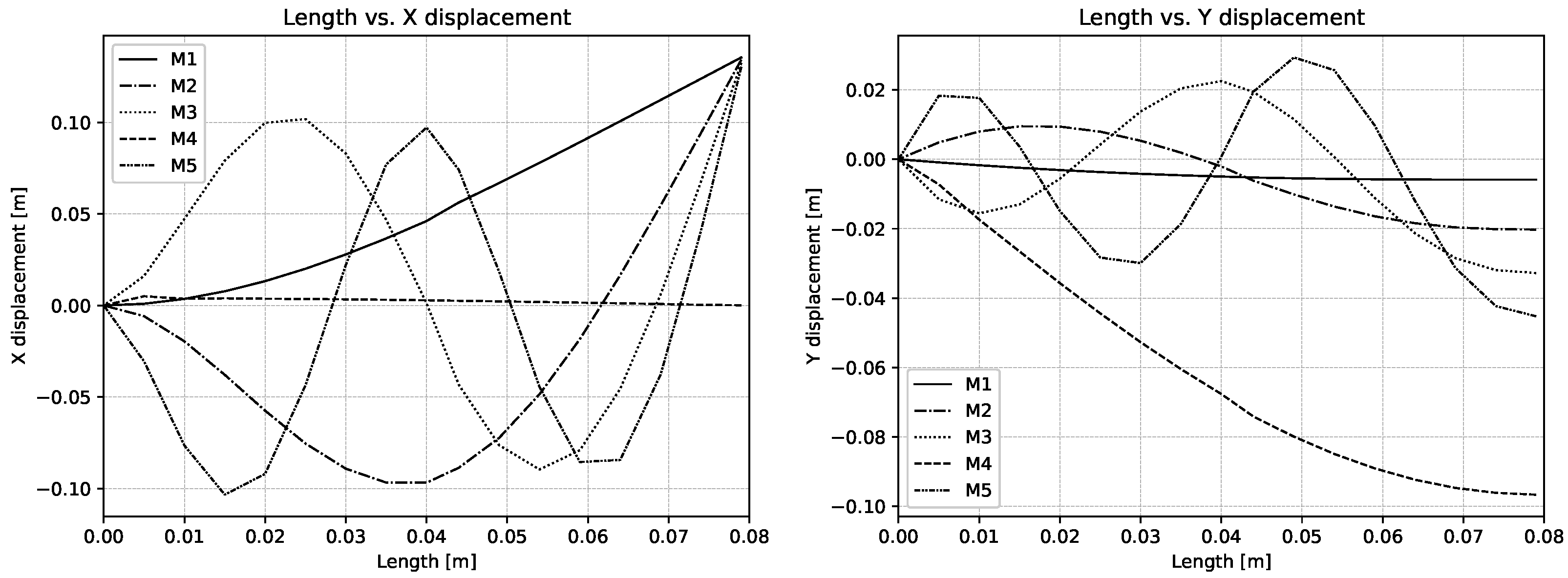
In this paper, vibration modes are expressed using natural frequencies and mass-normalized mode shapes, as detailed in Section 2.2. Equations (10)–(15) encloses the force vector and the structural deformation of the system. The equation of motion for a single mode (Equation (
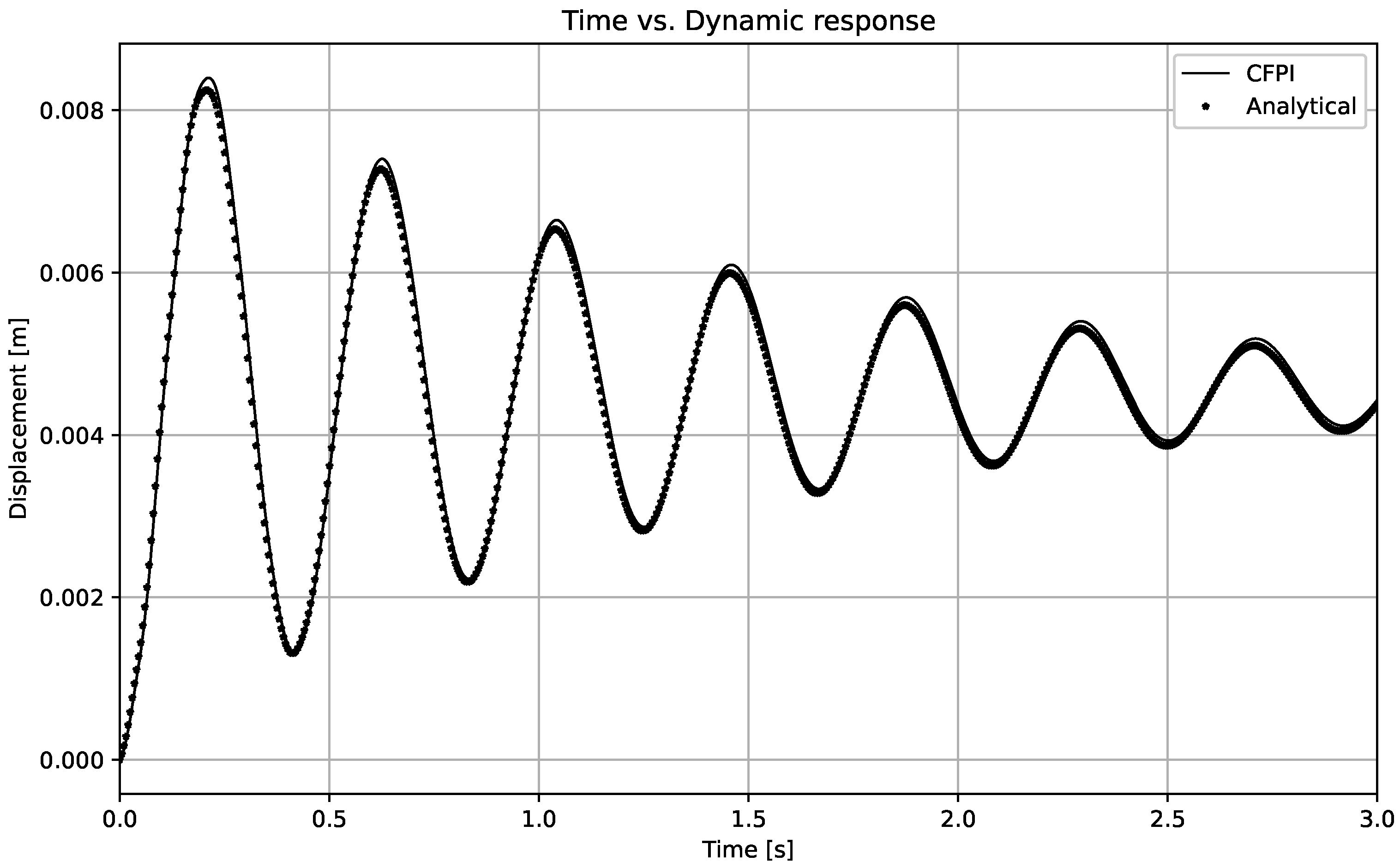
15)) is directly integrated in time within the fluid flow solver using the CFPI method, resulting in the generalized displacement, denoted y ( t ) . The same process is repeated for all modes at each time step of the simulation. Then, the global deformation of the structure is finally obtained using Equation (12), incorporating the calculated generalized displacement. Thereby ensuring that updated structural shape influences the flow calculations resulting in updated flow pressure and velocity fields [29]. Natural frequencies and corresponding modal vectors are determined externally before commencing the CFD, either by analytical methods or by using external modal solvers.
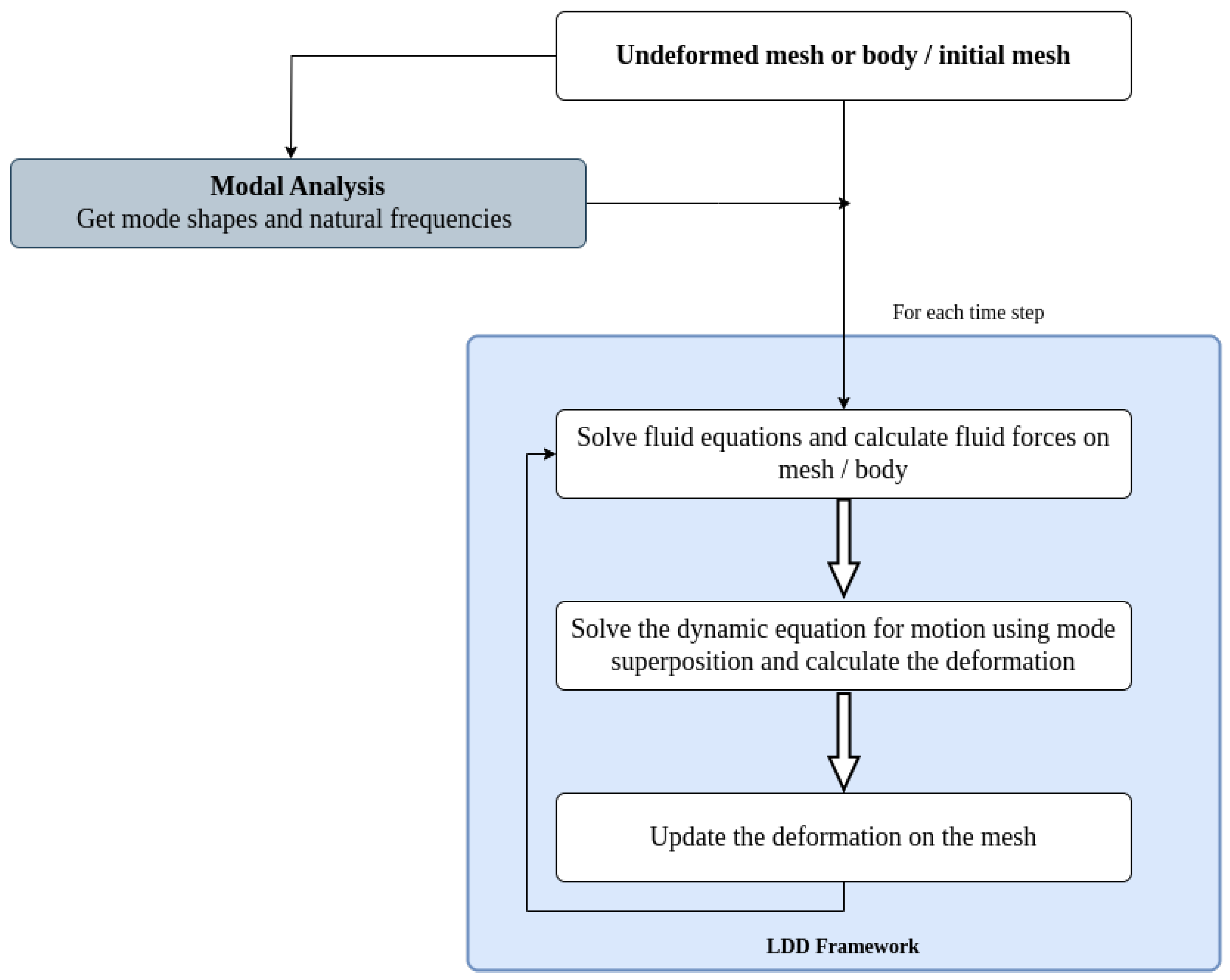
The workflow of the fluid–structure solver is depicted in Figure 1. The below steps are introduced to establish a two-way coupling of the fluid–structure interaction.
  • Calculate the mass-normalized mode shapes and corresponding natural frequencies, denoted as ω 1 , ω 2 , . . . , ω n .
  • Define the initial and boundary conditions for the simulation, including the initial displacement of the structural system if any.
  • Create Radial Basis Function (RBF) connections between fluid mesh and structural mesh to transfer the mode shape information if the structural mesh is not the same as the fluid mesh [40].
  • At every time step of the simulation Δ t :
    (a)
    Compute the forces exerted on the structural mesh due to fluid force.
    (b)
    Solve equation of motion (15) for each mode shapes and natural frequencies
    (c)
    Determine the overall deformation vector using Equation (12) and apply the resulting deformation to the mesh.
    (d)
    Solve the fluid equations for time t + Δ t , taking into account of structural deformation.
The coupling scheme based on the mode superposition method is formulated by solving the equation of motion with imposed loads by using mode shapes and natural frequencies which are determined from the modal analysis in the pre-calculation stage (step 1). This modal coupling is integrated into the LDD method, which takes initial and boundary conditions (step 2) from simulation input. This step is needed only in situations where the fluid mesh vertices do not overlap with structural vertices. In such a case, an interpolation is needed to compute the mode shape for the fluid mesh, based on the structural mesh (step 3). The displacement resulting from fluid forces (step 4a) is calculated within the modal coupling algorithm using CFPI method (step 4b). This deformation is applied on the mesh to account for geometric changes for the fluid solver (step 4c), consequently calculating the updated flow pressure and velocity fields using updated mesh (step 4d).

4. Results and Discussion

4.1. Validation of the Flow and Structural Solvers

4.1.1. Sloshing in Cobiodal Tank

The LDD method is validated by comparing the numerically obtained results to the experimental data from one of the Rhee test cases [41]. Rhee’s experimental setup uses a simplified cuboidal tank geometry with dimensions of 1200 mm, 600 mm, and 300 mm along the x, y, and z directions, respectively, and shown in Figure 2.
In this scenario, 20% of the tank volume is filled with water. The tank is subjected to a sinusoidal translation motion along the x-direction(swaying), characterized by an amplitude of 0.06 m and an oscillation period of 1.94 s. This study is based on the experimental work of Rhee [41] and aims to assess and confirm the agreement between the experimental and numerical outcomes for the specified tank geometry, flow properties and motion conditions with the LDD solver. The average pressure signal from the Rhee experiment at sensor location P1 (570 mm in the x-direction from the origin), is compared to the simulation average pressure and comparison plot shown in Figure 3. Also, the corresponding deviation is shown in Table 1.
The numerical results demonstrate a close correspondence with the experimental average impact pressure values at each sloshing peak obtained by the Rhee. This showcases the accuracy and reliability of the flow solver in predicting pressure values. Validating pressure loads is an important step in the modal superposition method. These loads serve as input parameters for calculating the deformation of the structure. Accurate validation ensures that the pressure loads used in the analysis are representative of the actual operating conditions and can provide reliable results. Any errors or inaccuracies in the pressure loads can lead to significant discrepancies in calculating the deformation of the structure. This, in turn, can impact its safety and performance. Therefore, it is crucial to validate the pressure loads through experimental or numerical methods to ensure the accuracy and reliability of the analysis results.

4.1.2. Cantilever Beam Vibration

To verify the implementation of a modal solver, a simple cantilever beam with a constant tip load applied over a time case is considered. An investigation was conducted to compute the dynamic behavior of a cantilever beam with specific geometric characteristics, including a length of 0.079 m and width of 0.005 m, under a 1N tip load and shown in Figure 4. This included the computation of the natural frequencies and their corresponding mode shapes. The initial five modes shapes are used in the simulation and shown in Table 2 and Figure 5.
For theoretical calculation, the damped vibration response of a cantilever beam which is subjected to a tip load (Figure 4) is calculated for various natural frequencies using Equation (19).
y ( t ) = i = 0 n F ω n i 2 1 e ζ ω n i t cos ( ω d i t )
where, y ( t ) is total displacement of the system at time t, F is magnitude of the load and n is number of natural frequencies. The term F ω n 2 scales the magnitude of the load. The exponential term e ζ ω n t accounts for the damping effect, causing the vibration to decay over time. The cosine term cos ( ω d t ) represents the oscillatory behavior of the system. ω n is natural frequency and ζ is damping ratio. Higher damping ratios ζ result in a larger reduction in vibration frequency. ω d is the damped angular frequency and it is calculated as follows
ω d = ω n 1 ζ 2
To understand the beam response more deeply, both theoretical and numerical methods were employed. The dynamic response of the system is mainly influenced by a few initial mode shapes. So all simulations were conducted exclusively for the initial five-mode shapes. The natural frequencies of a cantilever were used to calculate its theoretical displacement using Equation (19).
To compare this theoretical value with numerical simulations, the CFPI method was used to solve the dynamic equations of motion. The results were presented graphically in Figure 6. This comparison helped to understand the cantilever beam’s dynamic response better. The numerical simulation results closely match the theoretical predictions. The displacement difference is of the order of 1 × 10 4 , providing strong verification of the accuracy and reliability of the implementation. However, this is a simple load case, and more complex loading cases were validated in the upcoming section.

4.2. Deformation of Cantilever Gate

This section describes the initial experiment to verify the coupling implementation, which includes a slowly deforming cantilever beam. The deformation of the beam is induced by the transition from the hydrostatic loads into hydrodynamic loads. The verification of the coupling between flow and modal solver implementations is achieved by replicating an experiment originally conducted by Antoci et al. [42].
The experiment resembles the classic dam-breaking scenario, with gradual fluid loading on a rubber gate that is fixed to a rigid wall along its upper edge, which deforms under fluid forces. The experimental setup features a fluid column within a tank with dimensions: length ( A ) = 100 mm and height ( H ) = 140 mm. The rubber gate, supported by a rigid obstruction, extends downward to touch the floor. The height of the gate is L = 79 mm. For modeling, an elastic isotropic material with a density of ρ g a t e = 1100 kg/m3 and Young’s modulus E = 12 MPa is employed. The simulation considers only the first mode shape and its associated natural frequency. Validation is undertaken for the tank filled with water, density ρ = 1000 kg/m3 and dynamic viscosity μ = 10 3 Pa.s. Due to the pressure difference, the water flows through the rubber gate exerting the force to deflect it. The elastic deformation of the cantilever due to fluid loading is illustrated in Figure 7.
An assessment is being conducted to confirm whether the calculated deflection matches the expected magnitude, and to ensure the accuracy of the dynamic solver’s equations. The order of magnitude of deformation is the same as that in Antoci et al. [42]. However, this is not ideal for the primary objective of mode superposition. In this particular case, a static solution has been utilized, making the first bending mode sufficient for relevance and a small discrepancy in the predicted solution.

4.3. Elastic Baffle in Sloshing Tank

To investigate the impact of fluid–structure interaction with the complex cyclic load [43,44,45], an elastic baffle is introduced at the bottom of the tank, it is as same as the tank in Section 4.1.1 Figure 2. The tank is subjected to the same sinusoidal excitation with an amplitude of 0.06 m and a period of 1.94 s. In this study, the walls of the tank are assumed to be rigid, making the baffle the sole flexible component within the tank structure as shown in Figure 8.
The elastic baffle has dimensions of 5 mm, 150 mm, and 120 mm along the x, y, and z directions, respectively. The material property of the baffle includes the density of 4096 kg/m3, Young’s modulus of 38.4 MPa, and Poisson’s ratio of 0.3. The first five mode shapes were calculated from modal analysis and used for the simulation. Mode shapes are shown in Figure 9 and corresponding natural frequencies are shown in Table 3. By incorporating the elastic baffle model, the investigation aims to analyze and comprehend the effects of fluid–structure interaction within the tank system. Dimensions, material properties and displacement X at the location D1 (the top left corner of the baffle looking forward as shown in Figure 8) of the baffle are considered from the investigation conducted by Sampann [46]. The reference X-displacement is compared with the X-displacement obtained from the simulation and the results are presented graphically in Figure 10. The comparison shows that both results follow the same trend and also match closely at all the points where the most significant deformation takes place, thus verifying the precision of the modal coupling. At the peak, the deviation of deformation is minimal compared to the transition region where change in deformation takes place, due to the linear effect of mode superposition. The corresponding values are listed in Table 4. This provides an understanding of the baffle dynamic response under the specified sinusoidal excitation, which contributes added value to the present implementation of FSI.

4.4. Elastic Beam in Shallow Oil

The validity of the two-way coupling of fluid and structure has been substantiated through a comparison of both numerical simulations and experimental data obtained from benchmark studies conducted by Idelsohn et al. [47,48]. The experiments centered around the flexible beam exposed to sloshing loads and it is similar to Section 4.3 with different fluid properties and tank. Specifically, a cuboidal tank featuring a clamped elastic beam, made using dielectric polyurethane and filled with sunflower oil was investigated.
For the validation study, a specific test case from Idelsohn et al.’s work was selected. In this test case, the tank was filled with oil up to the height of the beam. The tank dimensions were 609 mm, 344.5 mm, and 39 mm in the x, y, and z directions, respectively. The flexible beam clamped to the tank’s bottom, exhibited dimensions of 4 mm, 57.4 mm, and 33.2 mm in the x, y, and z directions as shown in Figure 11. The beam is characterized by a density of 1100 kg/m3, a Young modulus of 60 MPa, and a Poisson ratio of 0.49. On the other hand, the oil has a density of 917 kg/m3 and a kinematic viscosity of 5 × 10 5 m²/s. The first five mode shapes obtained from modal analysis are used for the simulation. Mode shapes are presented in Figure 12 and corresponding natural frequencies are shown in Table 5.
The dynamic excitation imposed on the tank involved sinusoidal oscillatory motion about the z-axis, characterized by an amplitude of 4 degrees and a frequency of 0.61 Hz. Figure 13 shows X-displacement data at the tip of the beam, which has been compared with both experimental and numerical data from Idelsohn et al. The comparison indicates a favorable agreement between the results of the current study and the existing data [47]. Although a slight offset has been observed in certain locations, it matches closely with the numerical results from Idelsohn at the maximum deformation locations with a deviation order of 1 × 10 4 . The validation results consistently demonstrate a robust agreement in the accuracy of the implemented two-way coupling for fluid–structure interaction.

4.5. Flow Impact on a Cantilever Beam

After successful verification and validation of the FSI through various benchmark cases in the above Section 4.1, extending the exploration by conducting a study for a cantilever beam is subjected to sudden impact and subsequently oscillatory fluid loads. The geometric dimensions remain consistent with the static case, maintaining a thickness of 5 mm, while the fluid properties remain unchanged. The simulation involves a domain measuring 0.5 × 0.2 m, where an initial fluid column of dimensions 0.1 × 0.14 m is positioned at the left end of the domain. A beam is placed at the centerline of the tank, with its fixed end touching the bottom of the tank. The simulation replicates a scenario of a dam-break study, covering a total time of 10 s with intervals of 1 × 10 3 s.
In the simulation, the first five natural frequencies are utilized (as detailed in Table 2) along with their corresponding mode shapes that are illustrated in Figure 5. The dynamic behavior of the cantilever beam is presented in Figure 14.
The response of a beam to a load comes from any one individual mode shape or combination of mode shapes. From Figure 14, the combination of mode shape is clearly visible at 0.2 s and the dynamic response of the beam is dominated by the first mode after 5 s. The displacement of both the tip and mid-section of the beam is captured in the x and y directions, as shown in Figure 15. Figure 16 also shows the same behavior of combination mode shapes at 0.2 s and the dynamic response majorly from the first mode shape after 5 s. This observation highlights the effectiveness of the mode superposition technique in accurately capturing the impact of various modes on the system’s response.

4.6. Water Entry of a Wedge

The investigation on free fall of a wedge in the water case was replicated from the study carried out by Hosseinzadeh [49]. The wedge had a V-shaped variable dead-rise angle at the bottom. The wedge had dimensions of 1500 × 940 × 450 mm in length, breadth and depth. To reinforce the bottom of the wedge, 4 mm thick T−shaped stiffeners (T54 × 3 + 35 × 4 mm) were placed in the middle of the longitudinal and transverse direction on the starboard keel.
The material properties of the wedge were also taken into account, i.e., the wedge was modeled by using a material with density of 2700 kg/m3, the modulus of elasticity of 68 GPa, and the Poisson’s ratio of 0.33. The accuracy of the properties were important to consider, as they can have a significant effect on the behavior of the wedge during the free fall water entry [49]. The tank has dimensions of 5 × 5 × 1.75 m and is filled with water up to a height of 1.5 m in the z direction, as shown in Figure 17. For both structural modal analysis and fluid simulation, the surface mesh of the wedge was represented by 9200 triangles, which is shown in Figure 17. To conduct the numerical analysis of the impact loads, the wedge was dropped vertically from a height of 0.25 m (measured from the free surface up to the keel) into the water, with zero initial velocity. During the free fall, the velocity increased to U = 2.2 m/s as the wedge made contact with the water. The numerical time step was taken as constant, δ t = 2.5 × 10 3 . The modal analysis of the structural model resulted in obtaining the first five significant modes, which are shown in Figure 18 and corresponding natural frequencies are shown in Table 6. The same surface mesh and the modes obtained were used as input for the LDD-modal coupling solver.
During the simulation of free fall water entry, the evolution of loads and deformation of the wedge are observed and analyzed. The hydrodynamic pressure measured during the simulation at points PS1 and PP1 was compared with the experimental data given by Hosseinzadeh et al. [49] as shown in Figure 19. It shows that the maximum pressure matches with the experimental data and the deviation between them is 4%. However, it has been observed that the decrease in the pressure signal after the peaks happened faster in the simulation than that reported by the experimental data.
When the wedge impacts the water at a velocity of 2.2 m/s, it deforms in the X, Y, and Z directions. Figure 20 illustrates the deformation in the maximum impact load condition. It has been noted that the maximum amount of deformation observed was 36 μ m.

5. Conclusions

The modal-coupling solver has been seamlessly integrated into the Lagrangian Differencing Dynamics (LDD) solver. The numerical experimentation has shown that it enables effective two-way weak coupling of the fluid–structure interaction. The effectiveness of the Modal Coupling approach is attributed to its utilization of the mode superposition method. While the proposed bidirectional coupling is explicit in time, the insignificant cost of computing the structural deformation by using the mode superposition method allows the weak coupling to remain stable for time-steps that are required by the flow solver.
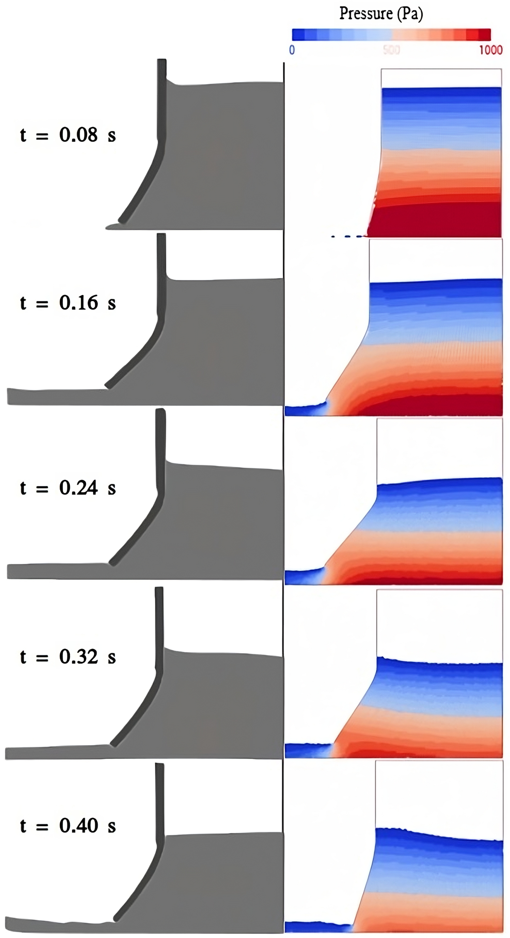
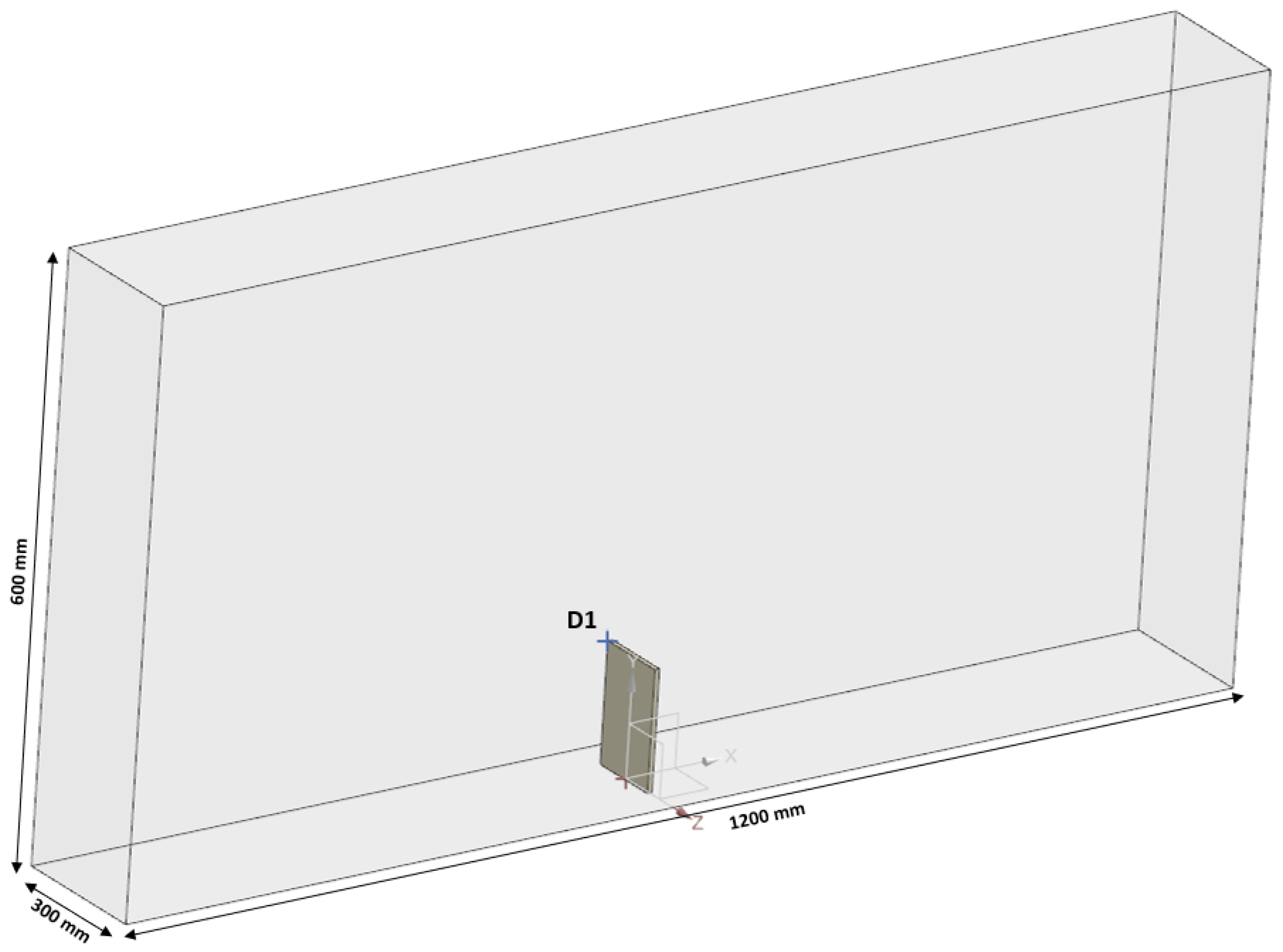
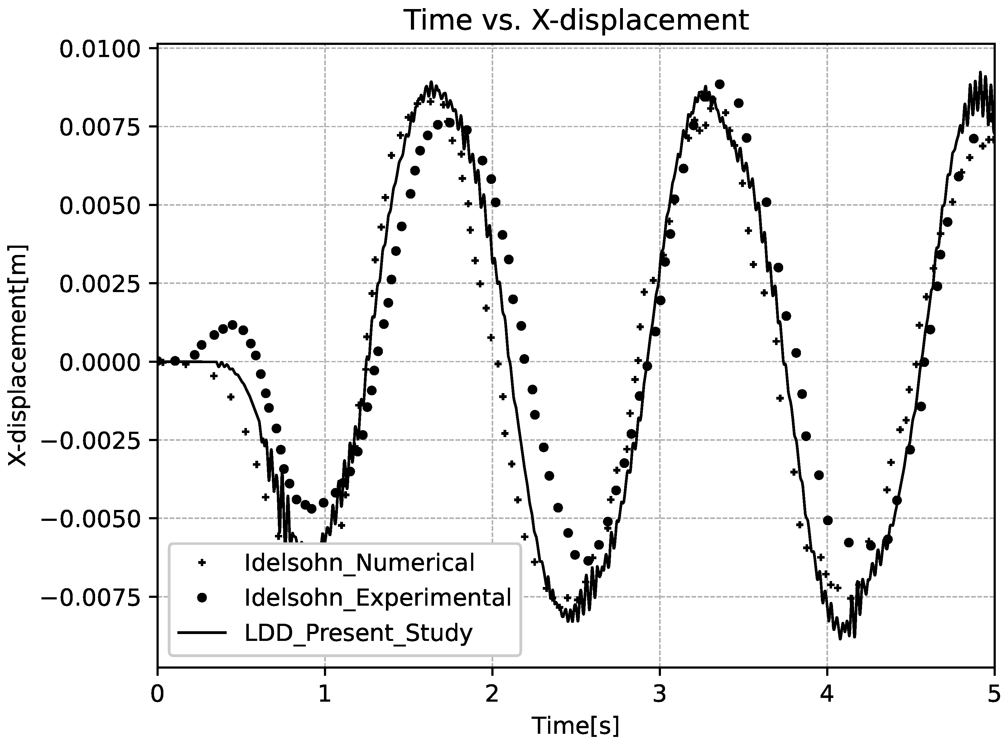
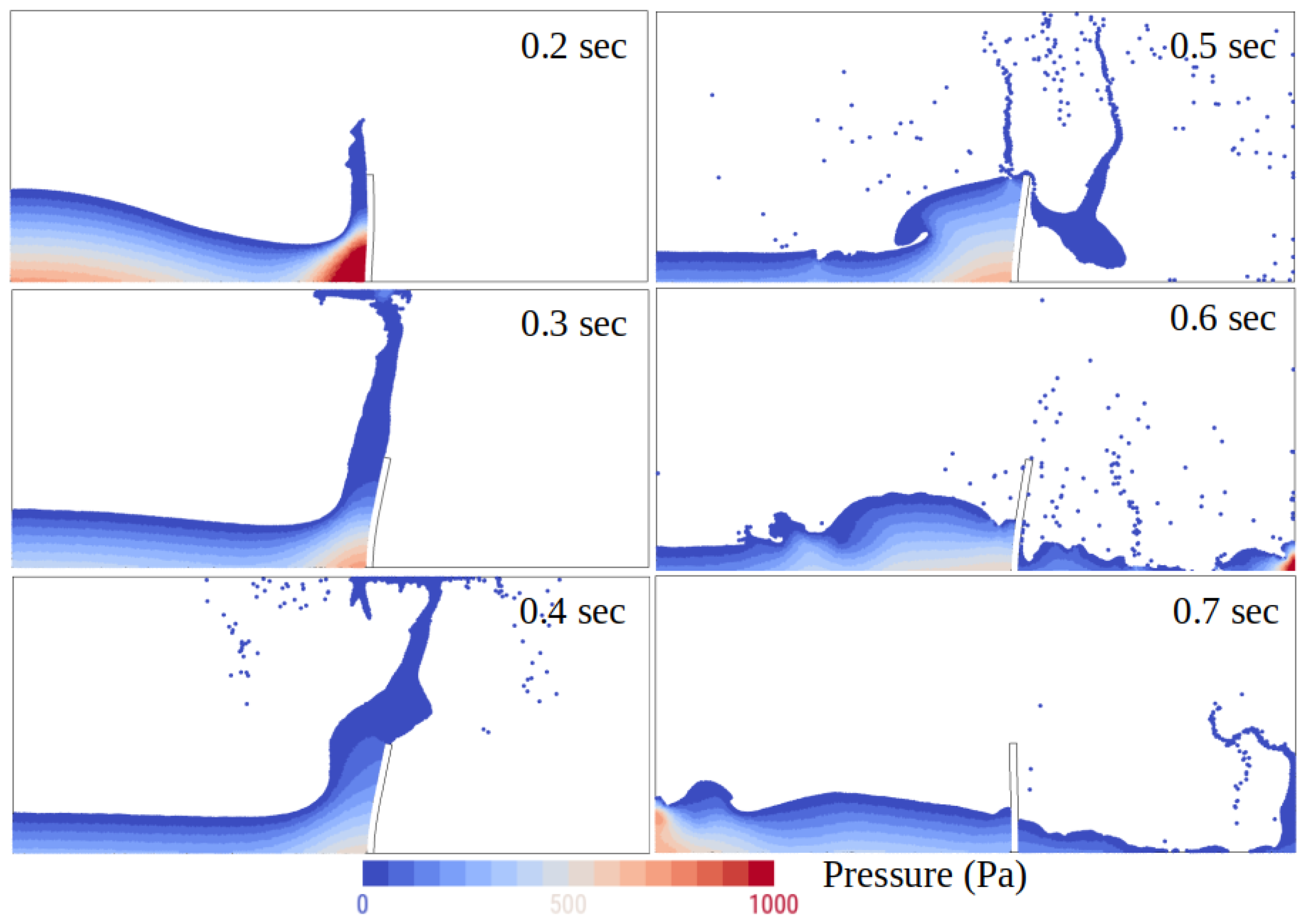
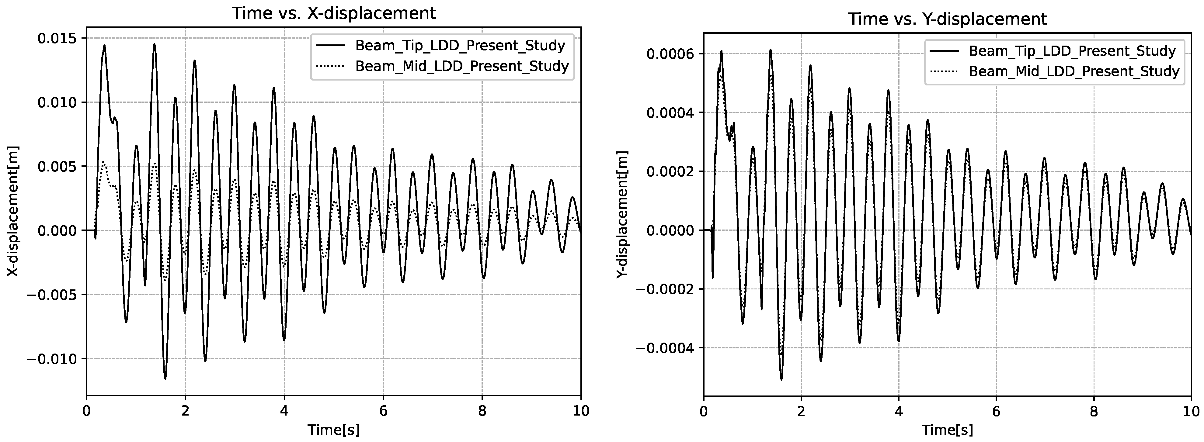
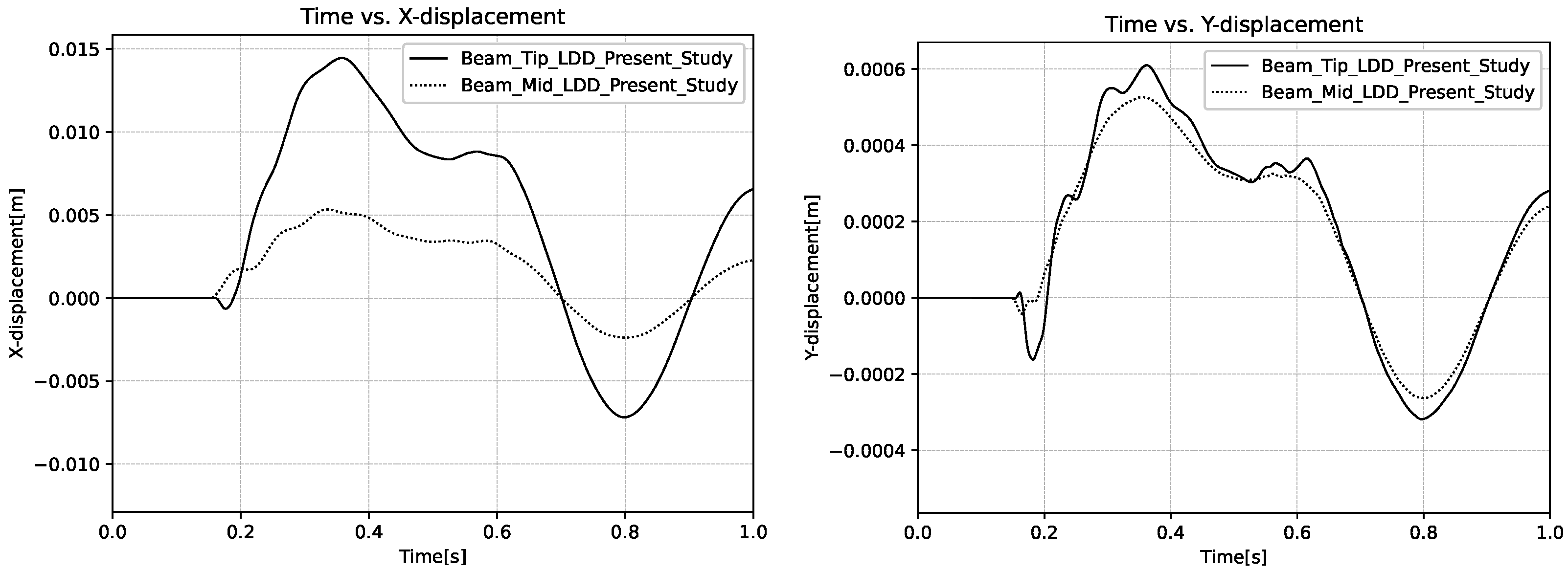
The verification and validation of the bidirectional fluid–structure interaction are successfully demonstrated through seven numerical experiments. The benchmark cases included both slowly and quickly deforming structures, and single or oscillatory fluid loads. The benchmark cases resembled swaying and rotating sloshing experiments (with and without flexible baffles), dam break experiments (with an elastic gate or obstacles) and water-entry experiment (slamming loads applied to a stiffened structure). The comparison between the numerically obtained results and the available experimental data demonstrated the ability of the proposed coupling method to capture complex interactions between fluids and structures.
The efficiency of the modal-coupling solver is accomplished by small computational cost of deforming the structure, by its flexibility to accommodate to the flow solver time-steps, and by using the Lagrangian LDD method to obtain accurate pressure loads. While this allows straightforward and efficient Lagrangian–Lagrangian coupling during the simulation, the engineering advantage is that there is no need for meshing or preparing the coupling interface, since the flow solver operates directly on surface meshes shared by the structural solver.
The above features of the proposed coupling method show practicality and applicability in future ship and offshore hydrodynamic simulations. The implementation process of the coupling scheme substantiates the tool’s capability to facilitate the effortless coupling of diverse solvers, all without necessitating changes to solver algorithms or input files. The incorporation of the energy equation into the framework is planned in future work. This expansion aims to explore the influence of energy on the fluid–structure interaction, thereby broadening the scope and insights of the analysis.

Author Contributions

Conceptualization, M.P. and J.B.; methodology, M.P. and J.B.; software, M.P.; validation, M.P.; investigation, M.P.; writing—original draft preparation, M.P.; writing—review and editing, C.P., J.B. and N.D.; visualization, M.P.; funding acquisition, C.P. and N.D.; supervision, J.B., D.S. and Ž.L. All authors have read and agreed to the published version of the manuscript.

Funding

This study was funded by the Croatian Science Foundation under project IP-2020-02-8568. M.P. and C.P. acknowledge the financial support received from CELTIC-NEXT under project COA-CFD, ID C2021/1-11.

Institutional Review Board Statement

Not applicable.

Informed Consent Statement

Not applicable.

Data Availability Statement

The data presented in this study are available on request from the corresponding author.

Acknowledgments

This study has been fully supported by the Croatian Science Foundation under project IP-2020-02-8568.

Conflicts of Interest

The authors declare no conflicts of interest.

Abbreviations

The following abbreviations are used in this manuscript:
CFDComputational Fluid Dnamics
LDDLagrangian Differencing Dynamics
FSIFluid Structure Interaction
RANSReynolds-Averaged Navier–Stokes
URANSUnsteady Reynolds-Averaged Navier–Stokes
VOFVoluem Of Fluid
RBFRadial Basis Function
DESDetached Eddy Simulation
SPHSmooth Particle Hydrodynamic
FEMFinite Element Method
DEMDiscrete Element Method
MPSMoving Particle Semi-implicit
CFPIComplementary Function and Particular Integral
MDOFMulti-Degree-Of-Freedom
SDOFSingle-Degree-Of-Freedom
ODEOrdinary Differential Equation
DOFDegree-Of-Freedom
PBDParticle-Based Dynamics

References

  1. Huang, L.; Rena, K.; Lib, M.; Tuković, Ž.; Cardiff, P.; Thomas, G. Fluid–structure interaction of a large ice sheet in waves. Ocean. Eng. Ser. 2019, 182, 102–111. [Google Scholar] [CrossRef]
  2. Danielsen, F.; Sørensen, M.K.; Olwig, M.F.; Selvam, V.; Parish, F.; Burgess, N.D.; Hiraishi, T.; Karunagram, V.M.; Rasmussen, M.S.; Hansen, L.B.; et al. The Asian tsunami: A protective role for coastal vegetation. Science 2005, 310, 643. [Google Scholar] [CrossRef] [PubMed]
  3. Zhou, W.; Wu, Z.; Mevel, L. Vibration-based damage detection to the composite tank filled with fluid. Struct. Health Monit. 2010, 9, 433–445. [Google Scholar] [CrossRef]
  4. Chella, M.A.; Tørum, A.; Myrhaug, D. An overview of wave impact forces on offshore wind turbine substructures. Energy Procedia 2012, 20, 217–226. [Google Scholar] [CrossRef]
  5. Liang, L.; Baoji, Z.; Hao, Z.; Hailin, T.; Weijie, W. Hydrodynamic performance optimization of marine propellers based on fluid–structure coupling. Brodogradnja 2023, 74, 145–164. [Google Scholar] [CrossRef]
  6. Zhang, Z.; Sun, P.; Pan, L.; Zhao, T. On the propeller wake evolution using large eddy simulations and physics-informed space-time decomposition. Brodogradnja 2024, 75, 75102. [Google Scholar] [CrossRef]
  7. Jensen, J.J. Load and Global Response of Ships; Elsevier: Amsterdam, The Netherlands, 2001; pp. 268–271. [Google Scholar]
  8. Bašić, J.; Degiuli, N.; Blagojević, B.; Ban, D. Lagrangian differencing dynamics for incompressible flows. J. Comput. Phys. 2022, 462, 111198. [Google Scholar] [CrossRef]
  9. Kwang-JunPaik, A.; Pablo, M.; Carrica, A.; Donghee Lee, B.; Kevin, M. Strongly coupled fluid–structure interaction method for structural loads on surface ships. Ocean. Eng. 2009, 36, 1346–1357. [Google Scholar]
  10. Hron, J.; Turek, S. A monolithic FEM/multigrid solver for an ALE formulation of fluid–structure interaction with applications in biomechanics. Fluid–Struct. Interact. 2006, 53, 146–170. [Google Scholar]
  11. Hron, J.; Turek, S. A monolithic FEM solver for an ALE for- mulation of fluid–structure interaction with configuration for numerical benchmarking. In Proceedings of the European Conference on Computational Fluid Dynamics, Egmond aan Zee, The Netherlands, 5–8 September 2006. [Google Scholar]
  12. Rugonyi, S.; Bathe, K.J. On finite element analysis of fluid flows fully coupled with structural interactions. CMES 2001, 2, 195–212. [Google Scholar]
  13. Degroote, J.; Hojjat, M.; Stavropoulou, E.; Wüchner, R.; Bletzinger, K.U. Partitioned solution of an unsteady adjointnfor strongly coupled fluid–structure interactions and application to parameter identification of a one-dimensional problem. Struct. Multidiscip. Optim. 2013, 47, 77–94. [Google Scholar] [CrossRef]
  14. Degroote, J.; Haelterman, R.; Annerel, S.; Vierendeels, J. Coupling techniques for partitioned fluid–structure interaction simulations with black-box solvers. In Proceedings of the 10th MpCCI User Forum, Sankt Augustin, Germany, 17–18 February 2009; Fraunhofer Institute SCAI: Sankt Augustin, Germany, 2009; pp. 82–91. [Google Scholar]
  15. Lim, W.Z.; Xiao, R.Y.; Hong, T.; Chin, C.S. Partitioned methods in computational modelling on fluid–structure interactions of concrete gravity-dam. Comput. Informat. Sci. 2013, 6, 154. [Google Scholar] [CrossRef]
  16. Bašić, M.; Blagojević, B.; Klarin, B.; Bašić, J. Coupling of Non–Newtonian meshless flow with structural solvers. In Proceedings of the VII International Conference on Particle-Based Methods, PARTICLES, Hamburg, Germany, 4–6 October 2021. [Google Scholar]
  17. Bašić, J.; Degiuli, N.; Malenica, Š. Insight into Hydrodynamic Damping of a Segmented Barge Using Numerical Free-Decay Tests. J. Mar. Sci. Eng. 2023, 11, 581. [Google Scholar] [CrossRef]
  18. Seng, S.; Jensen, J.J.; Malenica, Š. Global hydroelastic model for springing and whipping based on a free-surface CFD code (OpenFOAM). Int. J. Nav. Archit. Ocean Eng. 2014, 6, 1024–1040. [Google Scholar] [CrossRef]
  19. Cardiff, P.; Karač, A.; De Jaeger, P.; Jasak, H.; Nagy, J.; Ivanković, A.; Tuković, Z. An Open-Source Finite Volume Toolbox for Solid Mechanics and Fluid-Solid Interaction Simulations; Elsevier Ltd.: Amsterdam, The Netherlands, 2018. [Google Scholar]
  20. Tuković, Z.; Karač, A.; Cardiff, P.; Jasak, H.; Ivanković, A. OpenFOAM Finite Volume Solver for Fluid-Solid Interaction. Trans. Famena XLII-3 2018, 42, 1–31. [Google Scholar] [CrossRef]
  21. Schillaci, E.; Favre, F.; Troch, P.; Oliva, A. Numerical simulation of fluid structure interaction in free-surface flows: The WEC case. J. Phys. Conf. Ser. 2021, 2116, 012122. [Google Scholar] [CrossRef]
  22. Fourey, G.; Oger, G.; Le Touzé, D.; Alessandrini, B. Violent fluid–structure interaction simulations using a coupled SPH/FEM method. IOP Conf. Ser. Mater. Sci. Eng. 2010, 10, 012041. [Google Scholar] [CrossRef]
  23. Yang, Q.; Jones, V.; McCue, L. Free-surface flow interactions with deformable structures using an SPH–FEM model. Ocean Eng. 2012, 55, 136–147. [Google Scholar] [CrossRef]
  24. Nunez-Ramirez, J.; Marongiu, J.; Brun, M.; Combescure, A. A partitioned approach for the coupling of SPH and FE methods for transient nonlinear FSI problems with incompatible time-steps. Int. J. Numer. Methods Eng. 2017, 109, 1391–1417. [Google Scholar] [CrossRef]
  25. Wu, K.; Yang, D.; Wright, N. A coupled SPH-dem model for fluid–structure interaction problems with free-surface flow and structural failure. J. Comput. Struct. 2016, 177, 141–161. [Google Scholar] [CrossRef]
  26. Nasar, A.M.A.; Rogers, B.D.; Revell, A.; Stansby, P.K. Flexible slender body fluid interaction: Vector-based discrete element method with Eulerian smoothed particle hydrodynamics. Comput. Fluids 2019, 179, 563–578. [Google Scholar] [CrossRef]
  27. Joseph, O.; Rogers Benedict, D. A fluid–structure interaction model for free-surface flows and flexible structures using smoothed particle hydrodynamics on a GPU. J. Fluids Struct. 2021, 104, 103312. [Google Scholar]
  28. Degroote, J. Partitioned simulation of fluid–structure interaction. Arch. Comput. Methods Eng. 2013, 20, 185–238. [Google Scholar] [CrossRef]
  29. Debrabandere, F.; Tartinville, B.; Hirsch, C.; Coussement, C. Fluid-Structure interaction using a Modal Approach. J. Turbomach. 2012, 134, 051043. [Google Scholar] [CrossRef]
  30. Sun, K.Z.; Zhang, G.Y.; Zong, Z.; Djidjeli, K.; Xing, J.T. SNumerical analysis of violent hydroelastic problems based on a mixed MPS—mode superposition method. Ocean. Eng. 2019, 179, 285–297. [Google Scholar] [CrossRef]
  31. CoGroth, R.; Biancolini, M.E.; Costa, E.; Cella, U. Validation of High Fidelity Computational Methods for Aeronautical FSI Analyses. In Engineering Toward Green Aircraft—CAE Tools for Sustainable Mobility; Springer International Publishing: Berlin/Heidelberg, Germany, 2020; Volume 92, pp. 29–70. [Google Scholar]
  32. Banks, J.W.; Henshaw, W.D.; Schwendeman, D.W.; Tang, Q. A stable partitioned FSI algorithm for rigid bodies and incompressible flow. Part I: Model problem analysis. J. Comput. Phys. 2017, 343, 432–468. [Google Scholar] [CrossRef]
  33. Tiwari, S.; Kuhnert, J. Finite pointset method based on the projection method for simulations of the incompressible Navier–Stokes equations. In Meshfree Methods for Partial Differential Equations; Springer: Berlin/Heidelberg, Germany, 2003; pp. 373–387. [Google Scholar]
  34. Drumm, C.; Tiwari, S.; Kuhnert, J.; Bart, H.J. Finite pointset method for simulation of the liquid–liquid flow field in an extractor. Comput. Chem. Eng. 2008, 32, 2946–2957. [Google Scholar] [CrossRef]
  35. Onate, E.; Perazzo, F.; Miquel, J. A finite point method for elasticity problems. Comput. Struct. 2001, 79, 2151–2163. [Google Scholar] [CrossRef]
  36. Peng, C.; Bašić, M.; Blagojević, B.; Bašić, J.; Wu, W. A Lagrangian differencing dynamics method for granular flow modeling. J. Comput. Geotech. 2021, 137, 104297. [Google Scholar] [CrossRef]
  37. Bašić, J.; Degiuli, N.; Malenica, Š.; Ban, D. Lagrangian finite-difference method for predicting green water loadings. Ocean Eng. 2020, 209, 107533. [Google Scholar] [CrossRef]
  38. Basic, J.; Degiuli, N.; Ban, D. A class of renormalised meshless Laplacians for boundary value problems. J. Comput. Phys. 2018, 354, 269–287. [Google Scholar] [CrossRef]
  39. Paneer, M.; Bašić, J.; Lozina, Ž.; Sedlar, D.; Peng, C. Elastic Behaviours of Linear Structure Using Modal Superposition and Lagrangian Differencing Dynamics. In Proceedings of the VIII International Conference on Particle-Based Methods PARTICLES 2023, Milan, Italy, 9–11 October 2023. [Google Scholar]
  40. De Boer, A.; van der Schoot, M.S.; Bijl, H. Mesh deformation based on radial basis function interpolation. J. Comput. Struct. 2007, 85, 784–795. [Google Scholar] [CrossRef]
  41. Rhee, S.H. Unstructured grid based Reynolds-averaged Navier–Stokes method for liquid tank sloshing. J. Fluids Eng. 2008, 127, 572–582. [Google Scholar] [CrossRef]
  42. Antoci, C.; Gallati, M.; Sibilla, S. Numerical simulation of fluid–structure interaction by SPH. J. Comput. Struct. 2007, 85, 879–890. [Google Scholar] [CrossRef]
  43. Eswaran, M.; Saha, U.K.; Maity, D. Effect of baffles on a partially filled cubic tank: Numerical simulation and experimental validation. Comput. Struct. 2009, 87, 198–205. [Google Scholar] [CrossRef]
  44. Sankar, S.; Ranganathan, R.; Rakheja, S. Impact of dynamic fluid sloshnloads on the directional response of tank vehicles. Veh. Syst. Dyn. 1992, 21, 385–404. [Google Scholar] [CrossRef]
  45. Nicolici, S.; Bilegan, R.M. Fluid structure interaction modeling of liquid sloshing phenomena in flexible tanks. Nucl. Eng. Des. 2013, 258, 51–56. [Google Scholar] [CrossRef]
  46. Arora, S.; Vasudevan, S.; Sasic, S.; Etemad, S. A Partitioned FSI methodology for analysis of sloshing-induced loads on a fuel tank structure. In Proceedings of the 6th European Conference on Computational Mechanics (ECCM 6), Glasgow, UK, 11–15 June 2018. [Google Scholar]
  47. Idelsohn, S.R.; Marti, J.; Souto-Iglesias, A.; Onate, E. Interaction between an elastic structure and free-surface flows: Experimental versus numerical comparisons using the PFEM. Comput. Mech. 2008, 43, 125–132. [Google Scholar] [CrossRef]
  48. Marcela, C.; Laura, B.; Mario, S.; Jorge, D. Numerical Modeling and Experimental Validation of Free Surface Flow Problems. Arch. Comput. Methods Eng. 2016, 23, 139–169. [Google Scholar]
  49. Hosseinzadeh, S.; Tabri, K. Free-fall water entry of a variable deadrise angle aluminium wedge: An experimental study. In Developments in the Analysis and Design of Marine Structures, 1st ed.; CRC Press: Boca Raton, FL, USA, 2021; p. 9. [Google Scholar]
Figure 1. FSI with LDD workflow: This flowchart explains the process of integrating weak coupling of the modal solver.
Jmse 12 00318 g001
Figure 2. Tank considered for sloshing to validate the simulation pressure with Rhee [41] Experiment pressure.
Jmse 12 00318 g002
Figure 3. Comparison of pressure from the simulation at P1 location (Refer to Figure 2) with Rhee experiment pressure [41].
Jmse 12 00318 g003
Figure 4. Cantilever beam subjected to the tip load is considered for comparative analysis of Mode Superposition: Theoretical vs. Numerical.
Jmse 12 00318 g004
Figure 5. Mode shape of the beam along the length, Left: X-Displacement and Right: Y-Displacement.
Jmse 12 00318 g005
Figure 6. Comparison between the numerical and theoretical dynamic response of beam.
Jmse 12 00318 g006
Figure 7. Comparison of cantilever beam deformation from the current study with Antoci et al. [42] at different time steps such as t = 0.08 s, 0.16 s, 0.24 s, 0.32 s and 0.40 s.
Jmse 12 00318 g007
Figure 8. Rhee sloshing tank is considered and an elastic baffle is introduced at the bottom of the tank.
Jmse 12 00318 g008
Figure 9. Modal results of an elastic baffle with reference to its undeformed wireframe, i.e., the first five mode-shapes.
Jmse 12 00318 g009
Figure 10. Comparison of X-displacement from the simulation at D1 location (Refer to Figure 8) with numerical results from Sampann [46].
Jmse 12 00318 g010
Figure 11. Idelsohn sloshing tank is considered and an elastic beam is introduced at the bottom of the tank.
Jmse 12 00318 g011
Figure 12. Modal results of an elastic beam with reference to its undeformed wireframe, i.e., the first five mode-shapes.
Jmse 12 00318 g012
Figure 13. Comparison of X-displacement from the simulation at the end of the beam (Refer to Figure 11) with experimental and numerical results from [47].
Jmse 12 00318 g013
Figure 14. Dynamic response of cantilever beam at different time step.
Jmse 12 00318 g014
Figure 15. Dynamic response over a time period at the mid and tip section, Left: X Displacement and Right: Y Displacement.
Jmse 12 00318 g015
Figure 16. Displacement at the mid and tip section until 1 s, Left: X Displacement and Right: Y Displacement.
Jmse 12 00318 g016
Figure 17. Numerical setup to replicate the experiment of [49]. On the left, a tank filled with water up to 1.5 m and a wedge placed at a distance of 0.25 m above the free surface. On the right, a wedge with a surface mesh was used for the modal coupling solver.
Jmse 12 00318 g017
Figure 18. Modal results of a wedge with reference to its undeformed wireframe, i.e., the first five mode shapes.
Jmse 12 00318 g018
Figure 19. Comparison of dynamic pressure from the simulation with experimental results from [49], Left: PS1 point as per [49] and Right: PP1 point as per [49].
Jmse 12 00318 g019
Figure 20. Deformation of Wedge in X, Y, and Z directions and deformation magnitude at maximum impact load condition, where wedge touches the water with 2.2 m/s velocity.
Jmse 12 00318 g020
Table 1. Deviation of pressure from the simulation with respect to Rhee Experiment at peak location.
Region1st Peak2nd Peak
Deviation of pressure [kPa]0.10.35
Table 2. Initial 5 Modes and natural frequencies of the cantilever beam.
Mode12345
Natural Frequency (Hz)15.0993.433257.66374.8495.57
Table 3. Initial 5 Modes and natural frequencies of the elastic baffle.
Mode12345
Natural Frequency (Hz)100.12270.05301.33392.05505.44
Table 4. Deviation of deformation from the simulation with respect to Sampann.
RegionPeakTransition
Max Deviation of deformation [m]0.0050.01
Table 5. Initial 5 Modes and natural frequencies of the elastic beam.
Mode12345
Natural Frequency (Hz)186.4560.61673.29856.07939.09
Table 6. Initial 5 Modes and natural frequencies of the wedge.
Mode12345
Natural Frequency (Hz)213.8376.6440.95529.12535.23
Disclaimer/Publisher’s Note: The statements, opinions and data contained in all publications are solely those of the individual author(s) and contributor(s) and not of MDPI and/or the editor(s). MDPI and/or the editor(s) disclaim responsibility for any injury to people or property resulting from any ideas, methods, instructions or products referred to in the content.

