
Assessment of Numerical Captive Model Tests for Underwater Vehicles: The DARPA SUB-OFF Test Case

Abstract
:1. Introduction
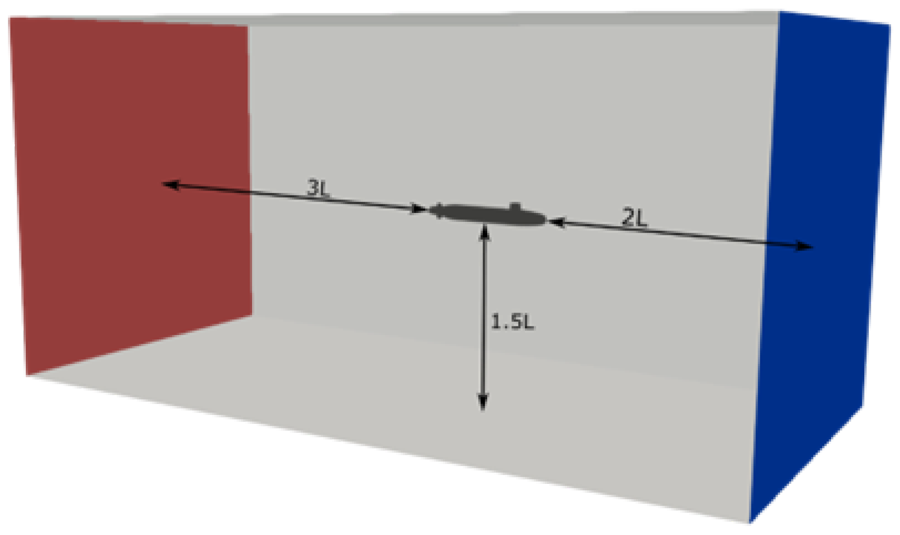
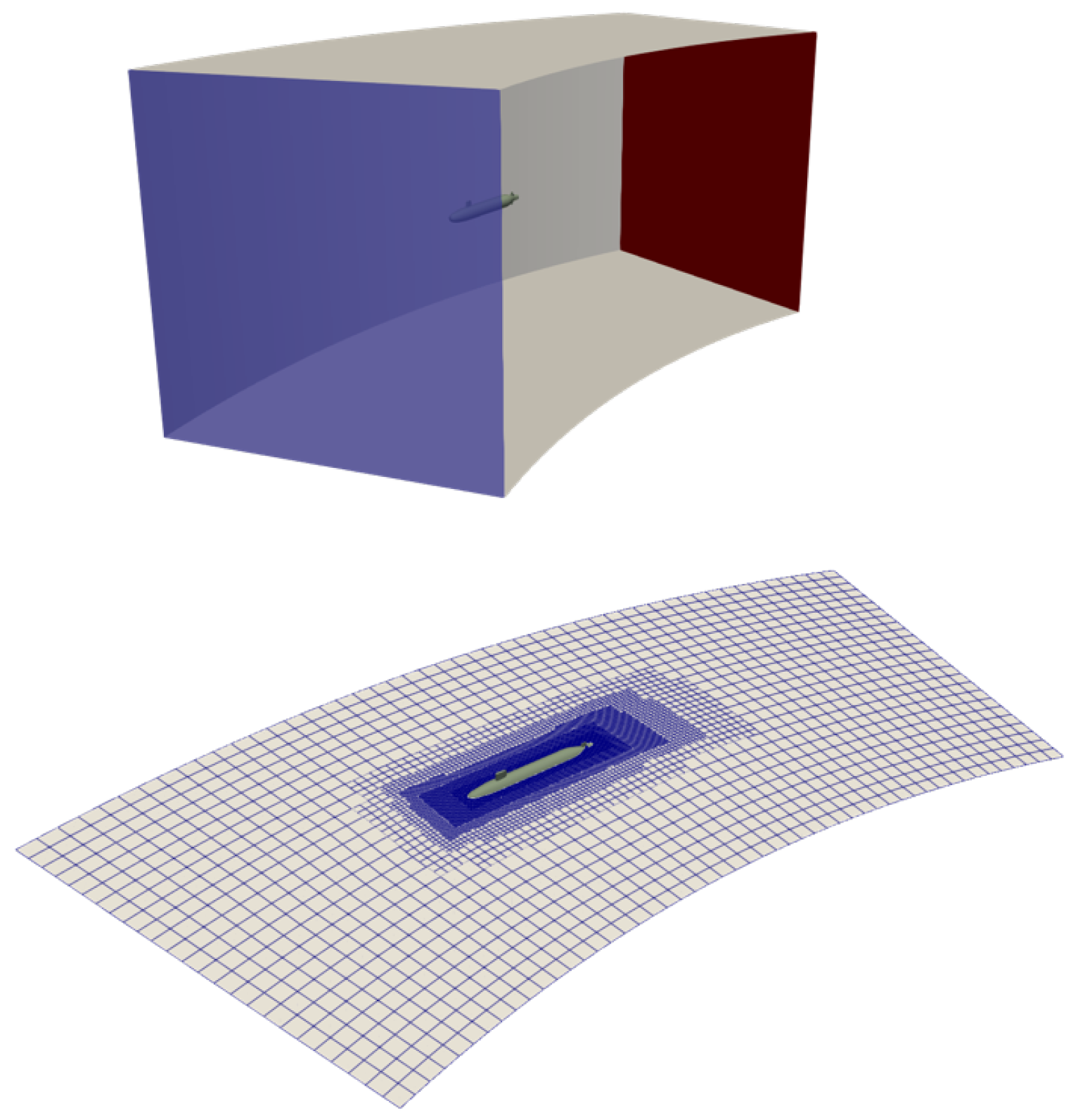
2. Computational Setup and Test Case
3. Numerical Model
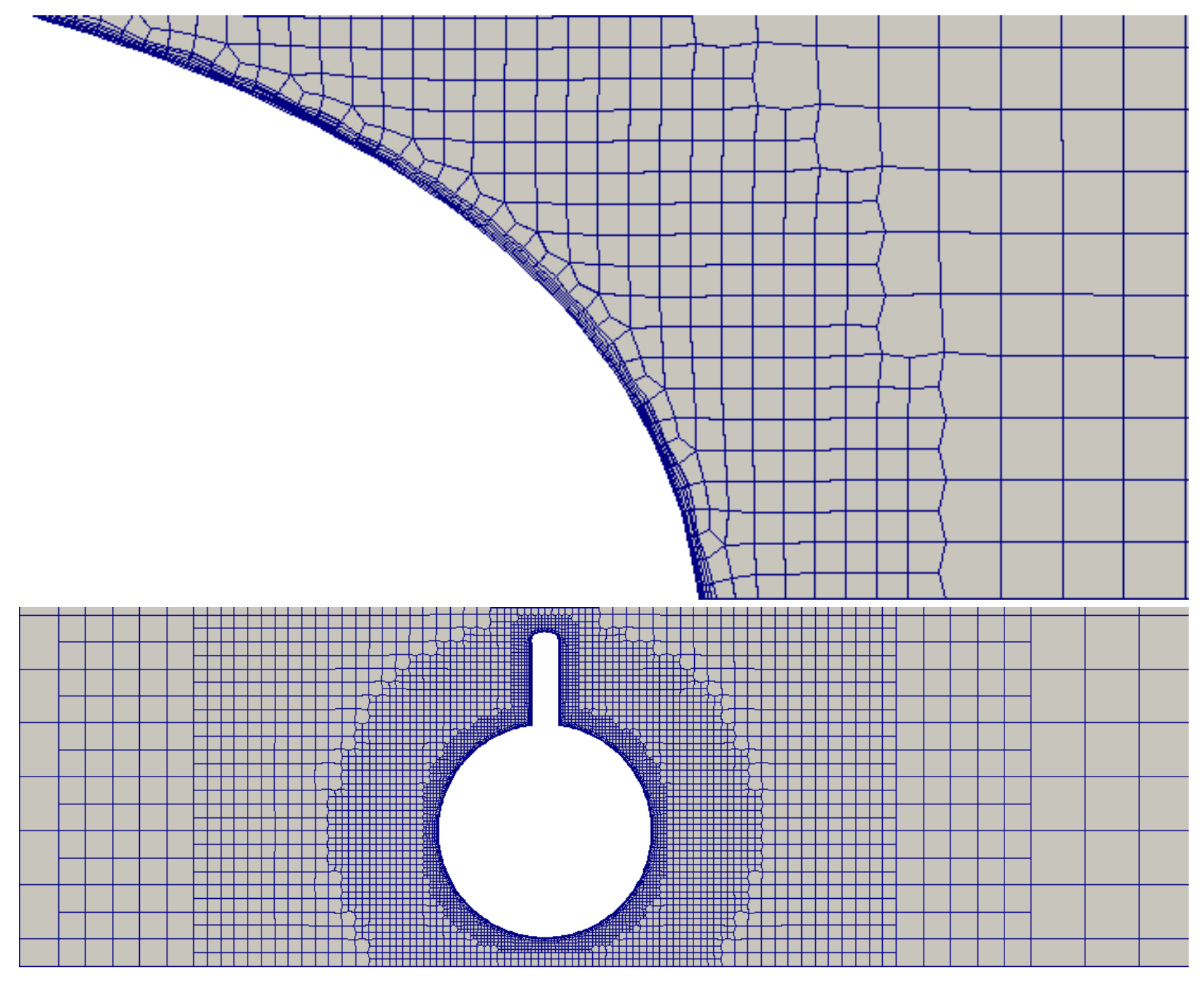
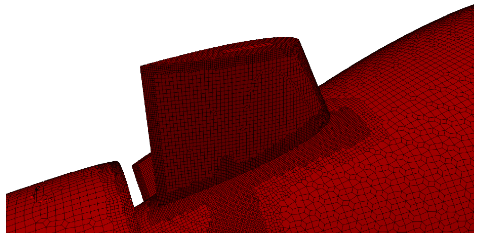
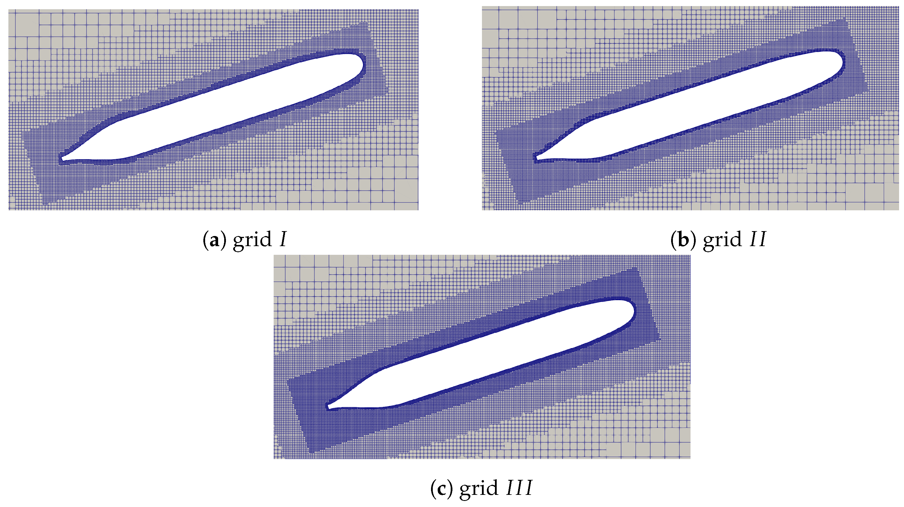
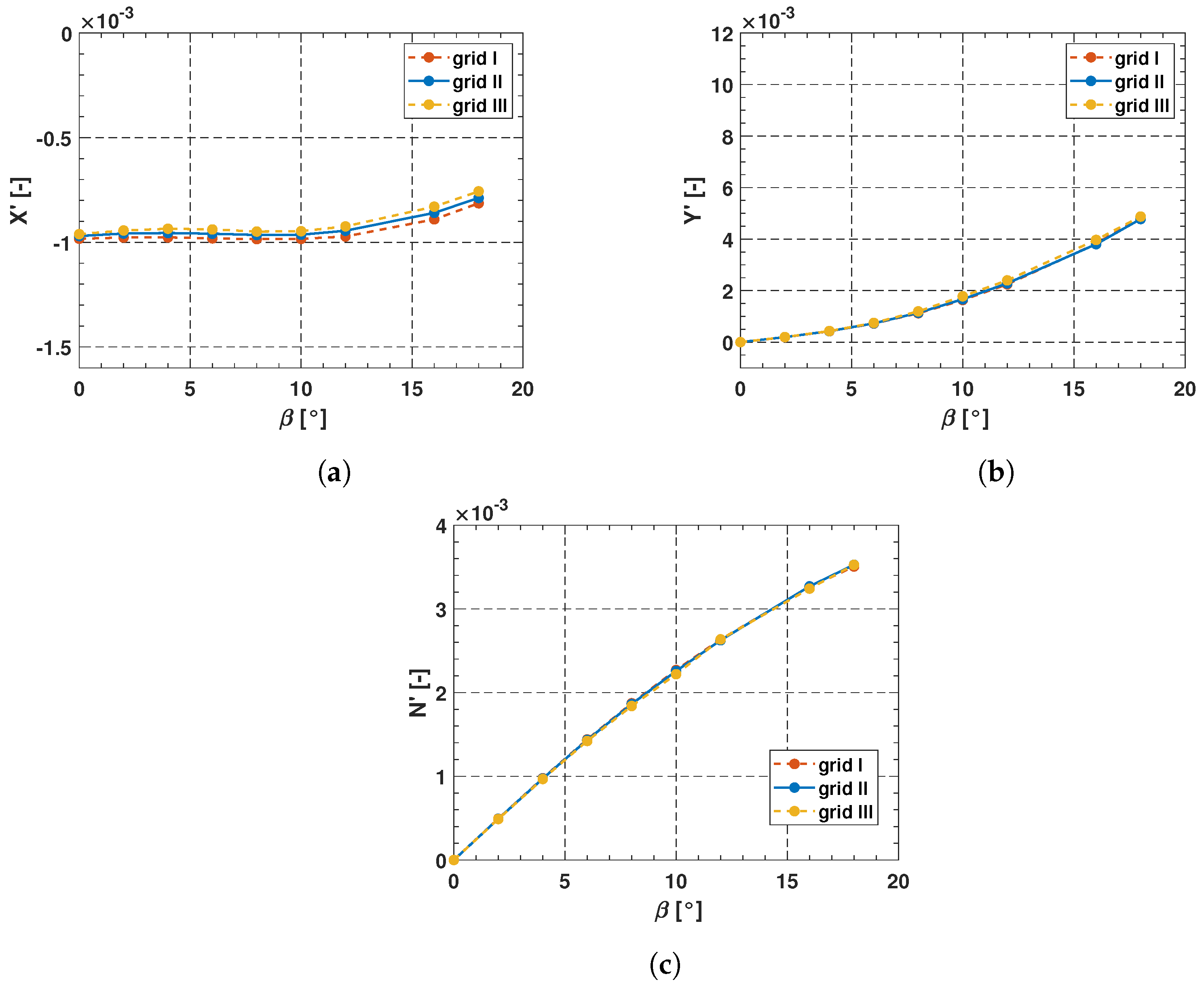
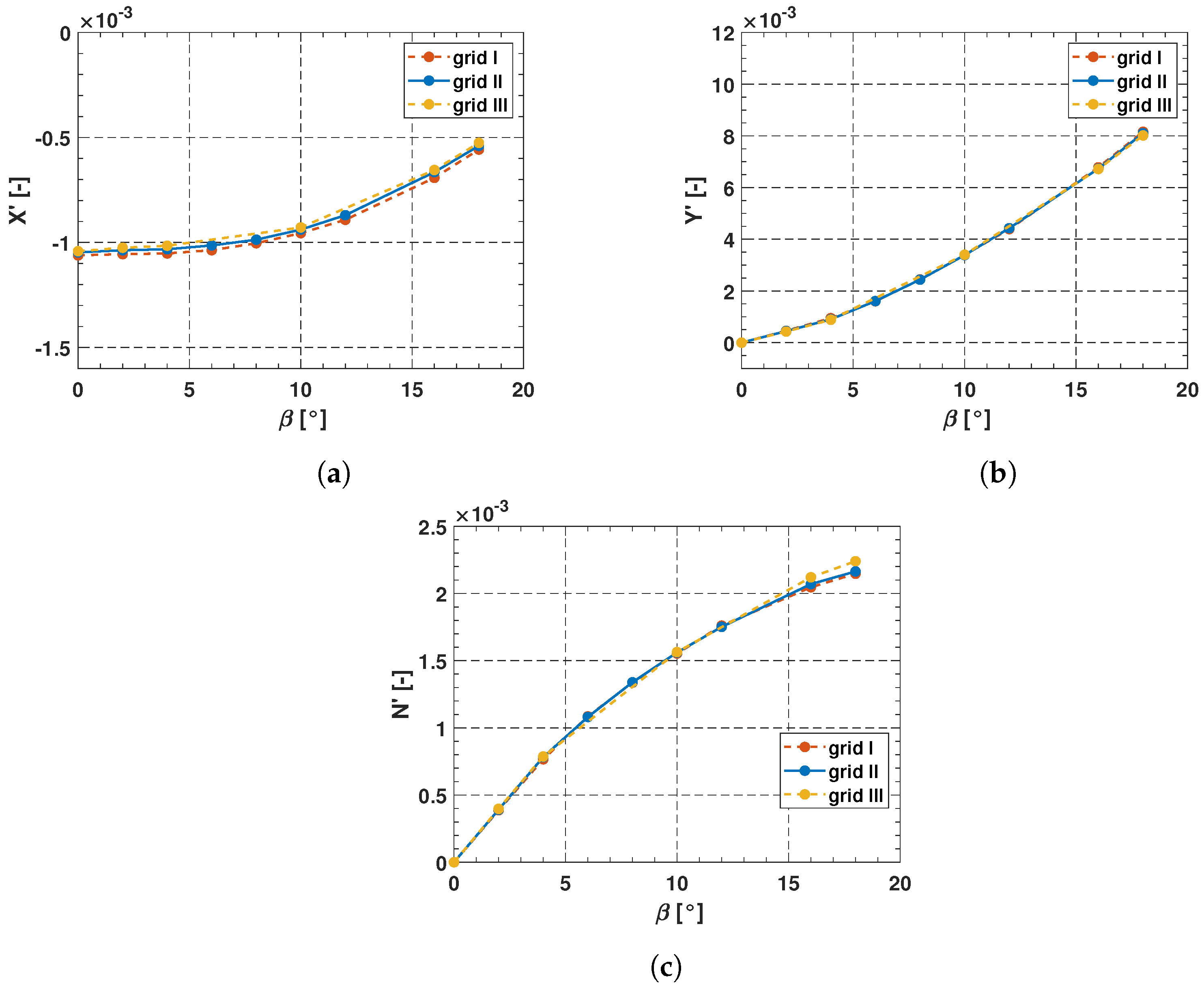
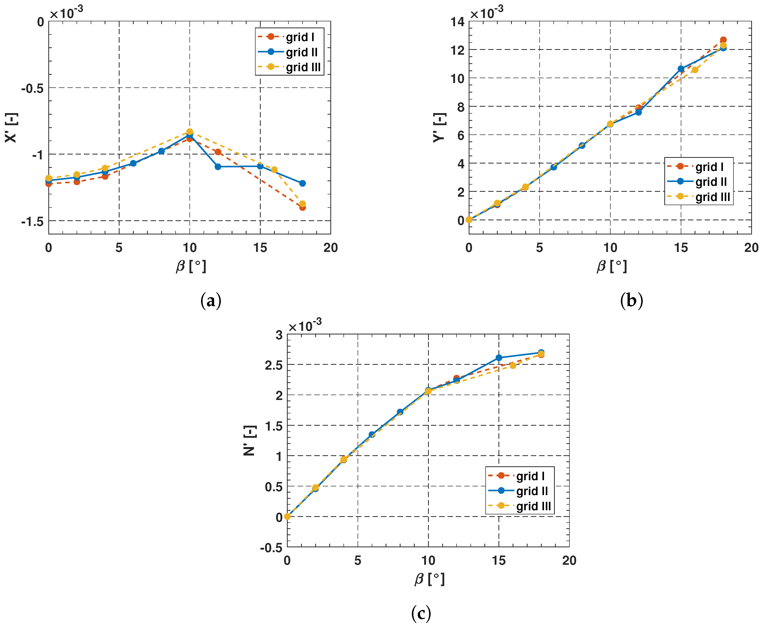
3.1. Mesh Sensitivity Analysis
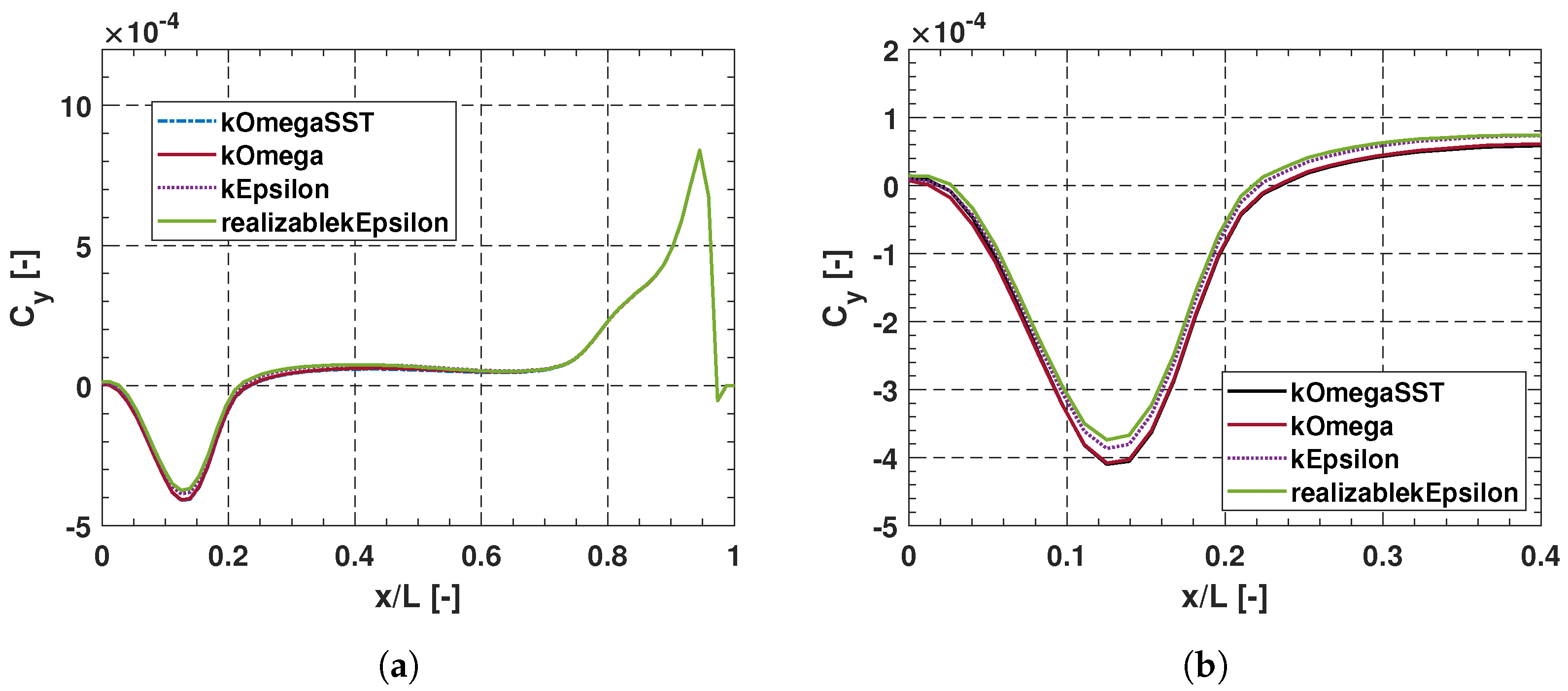
3.2. Turbulence Model Analysis
4. Results: Pure Drift Tests
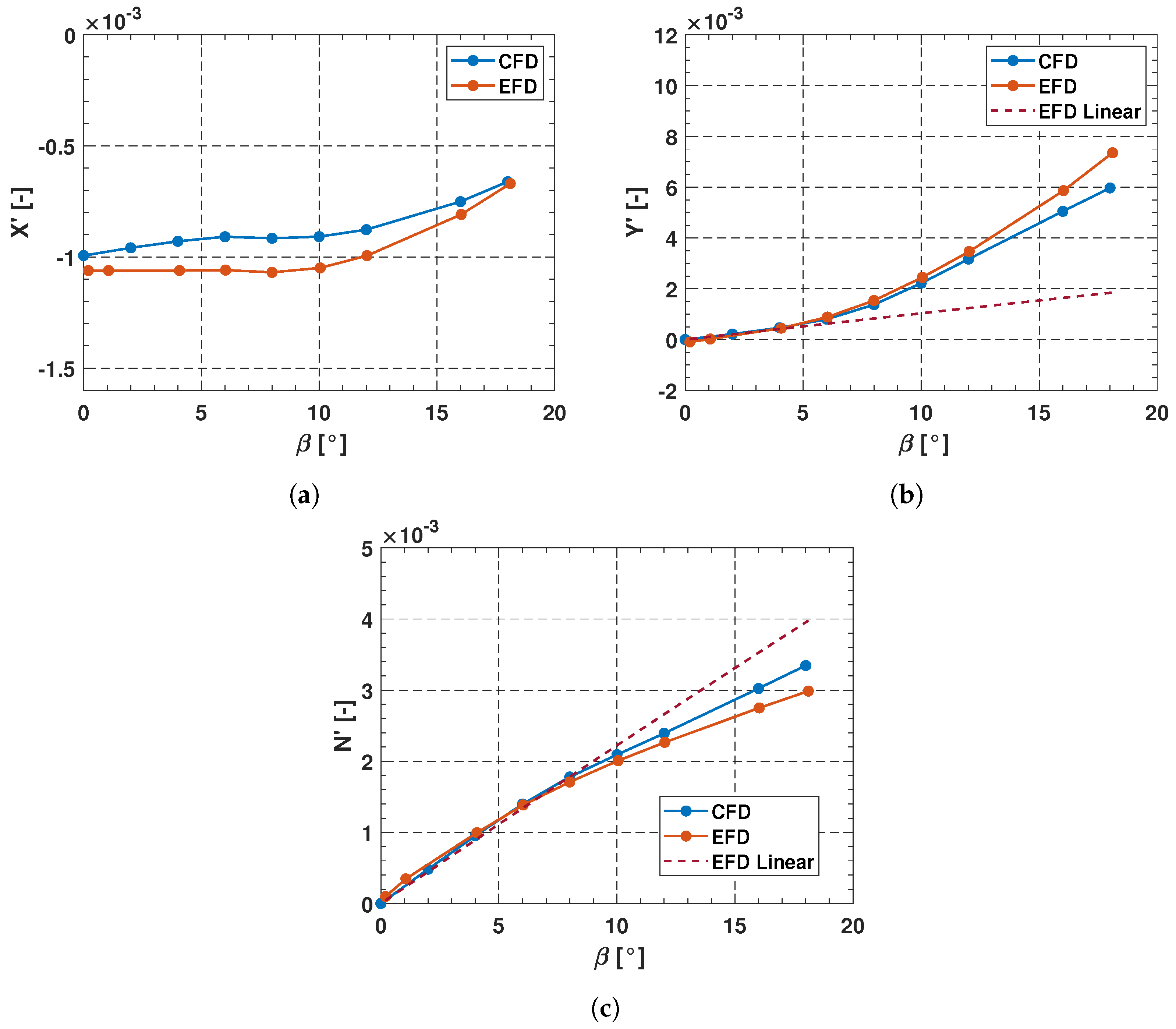
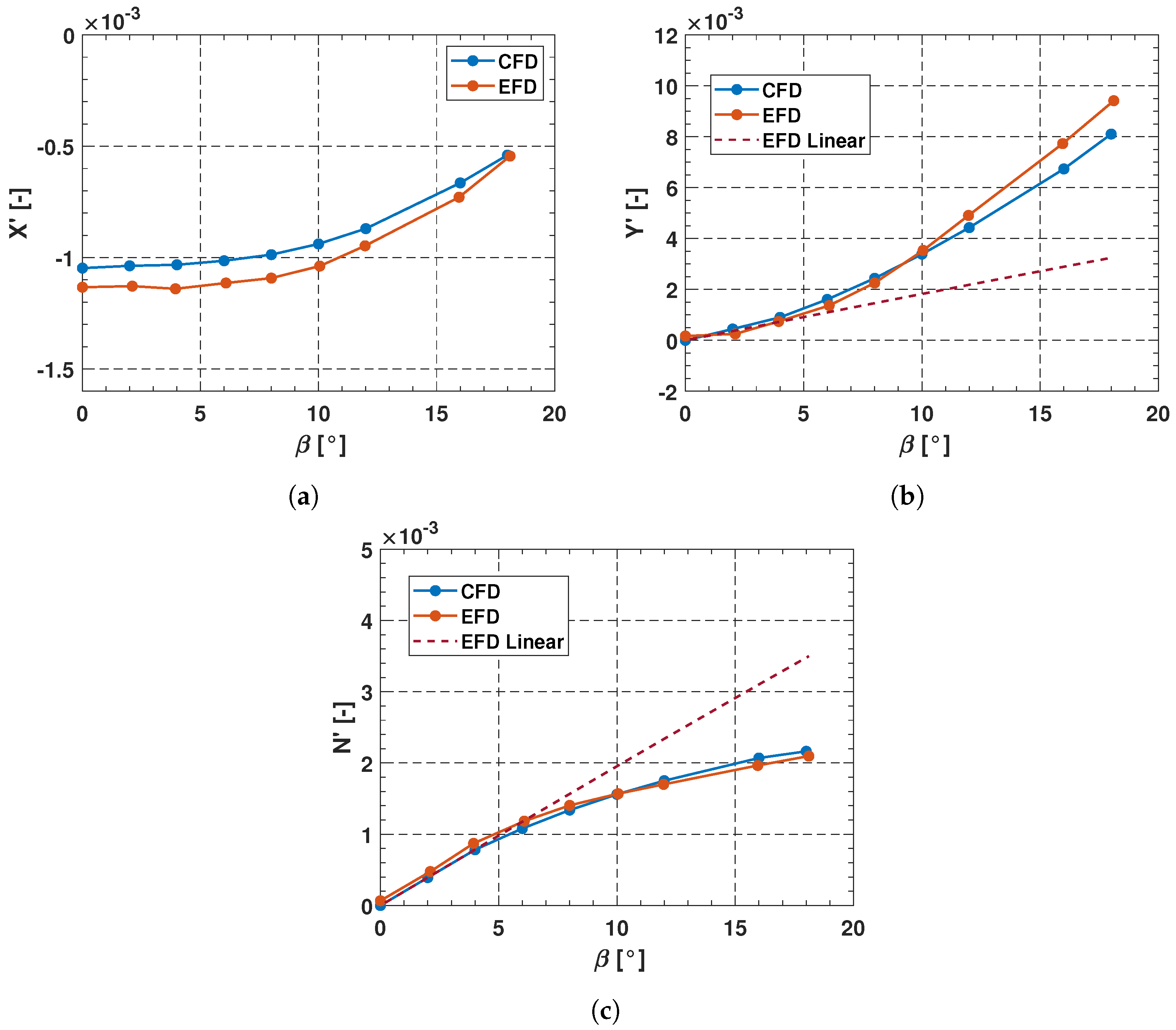
4.1. Barehull Configuration
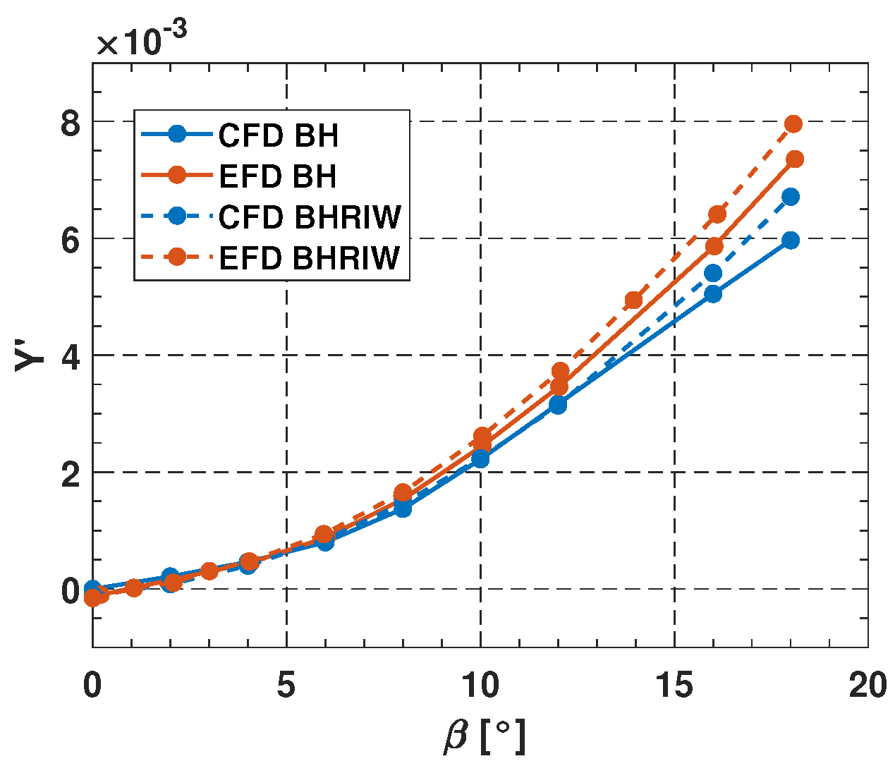
4.2. Barehull with Ring Wing
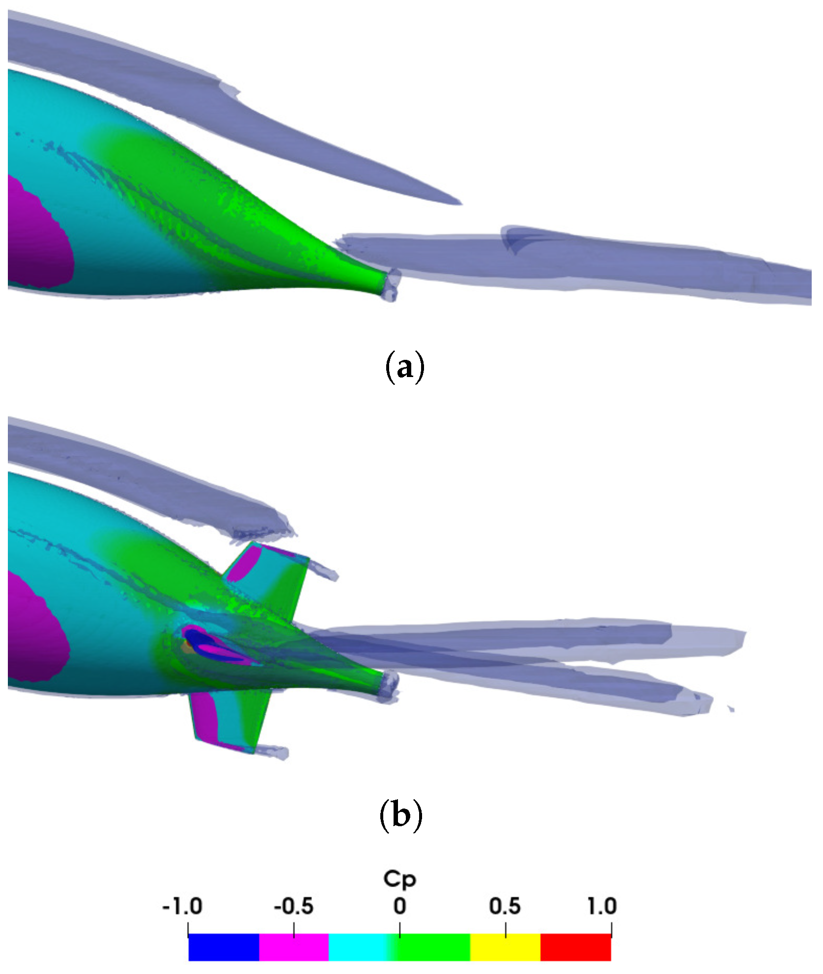
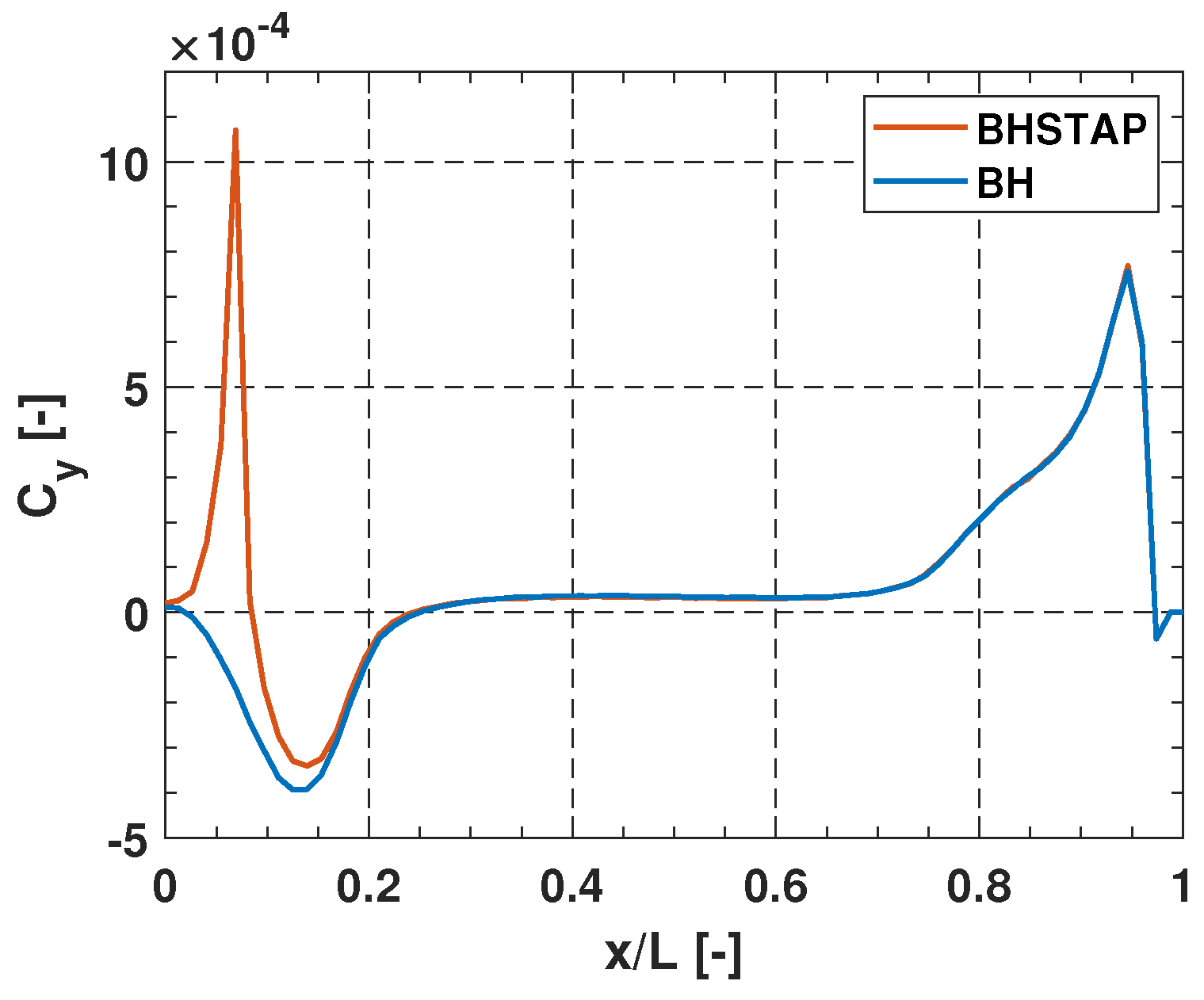
4.3. Barehull with Stern Appendages
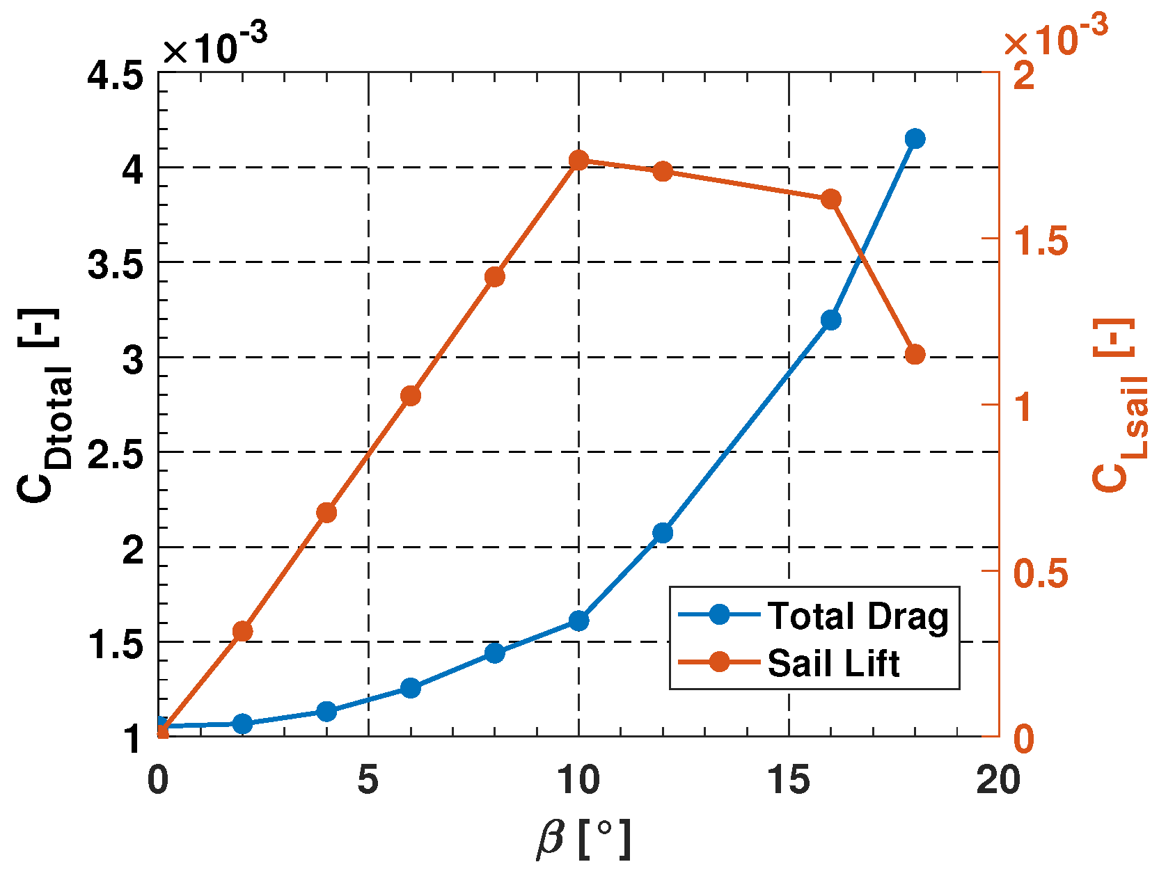
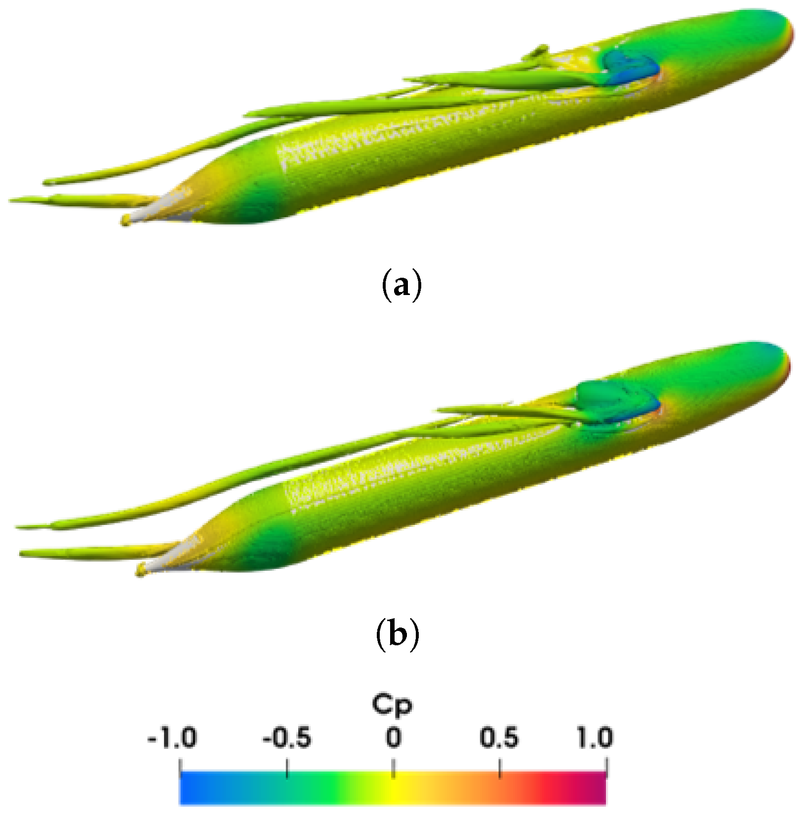
4.4. Barehull with Sail
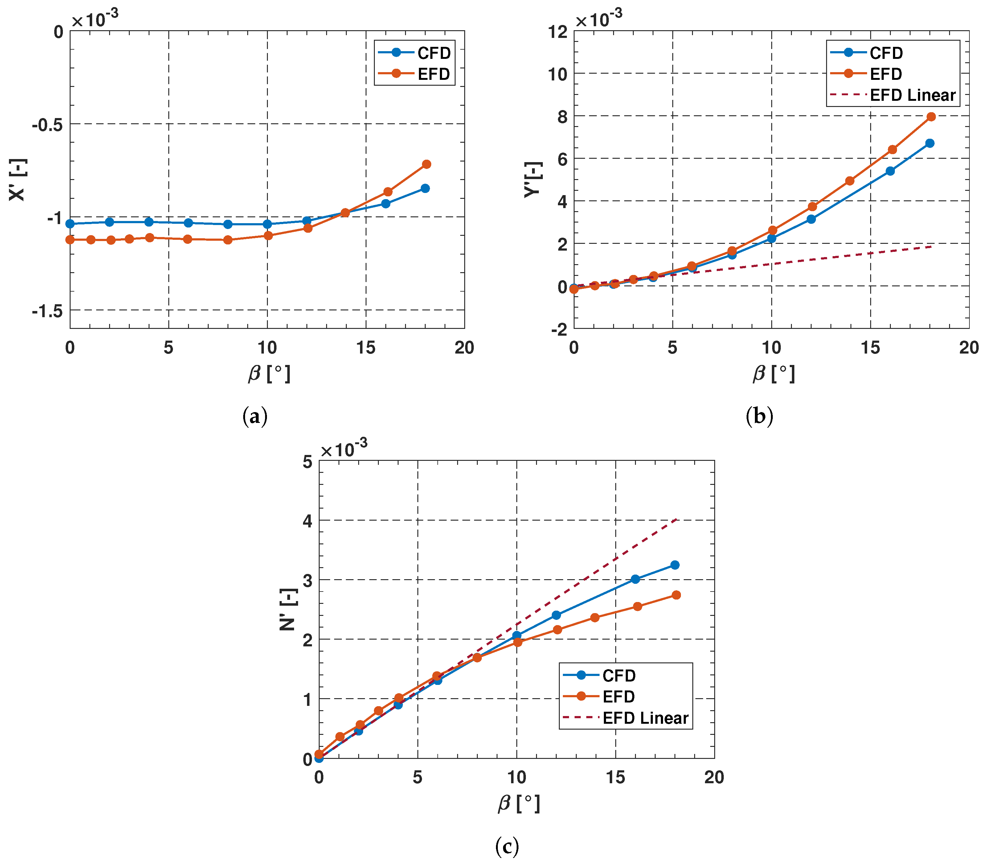
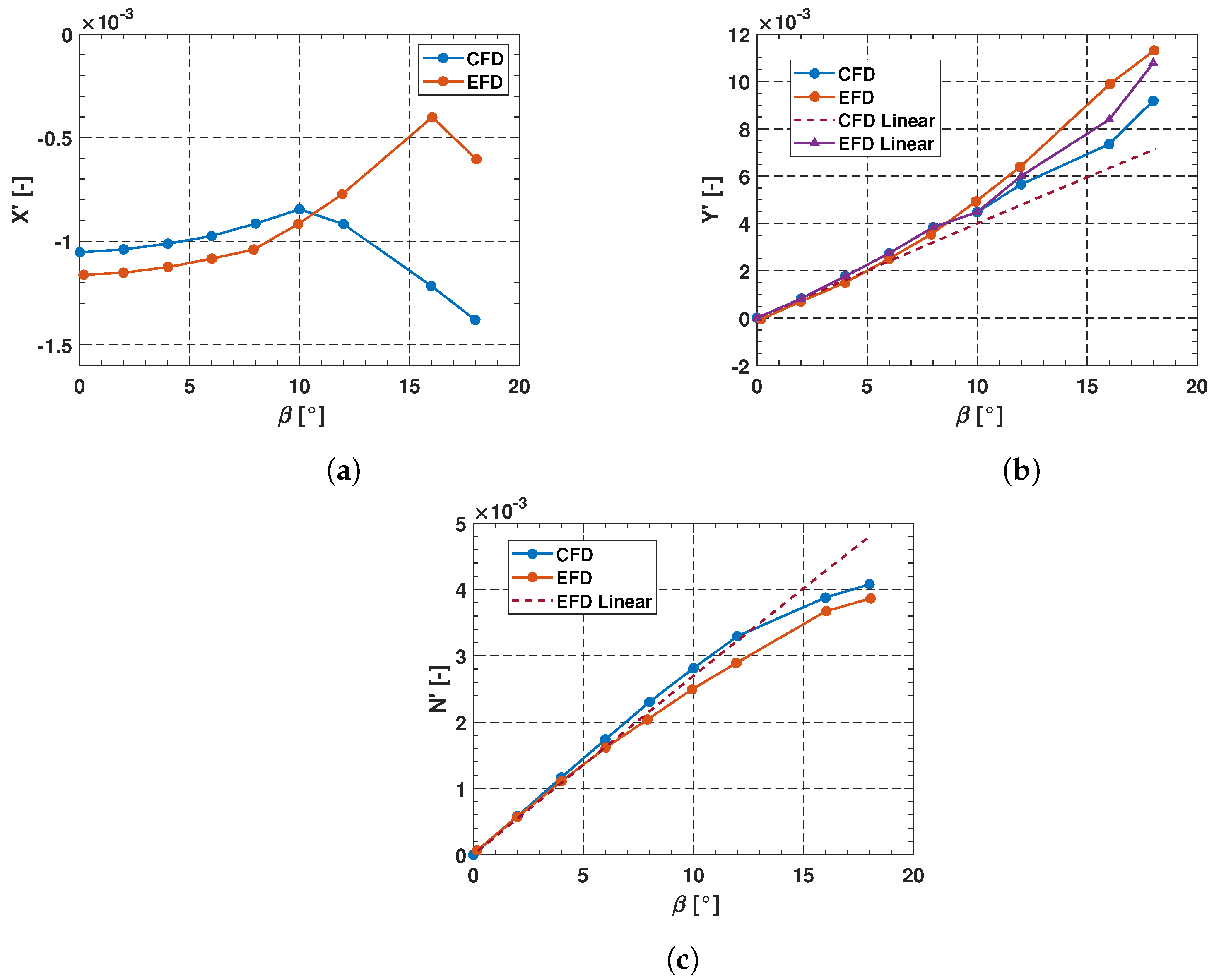
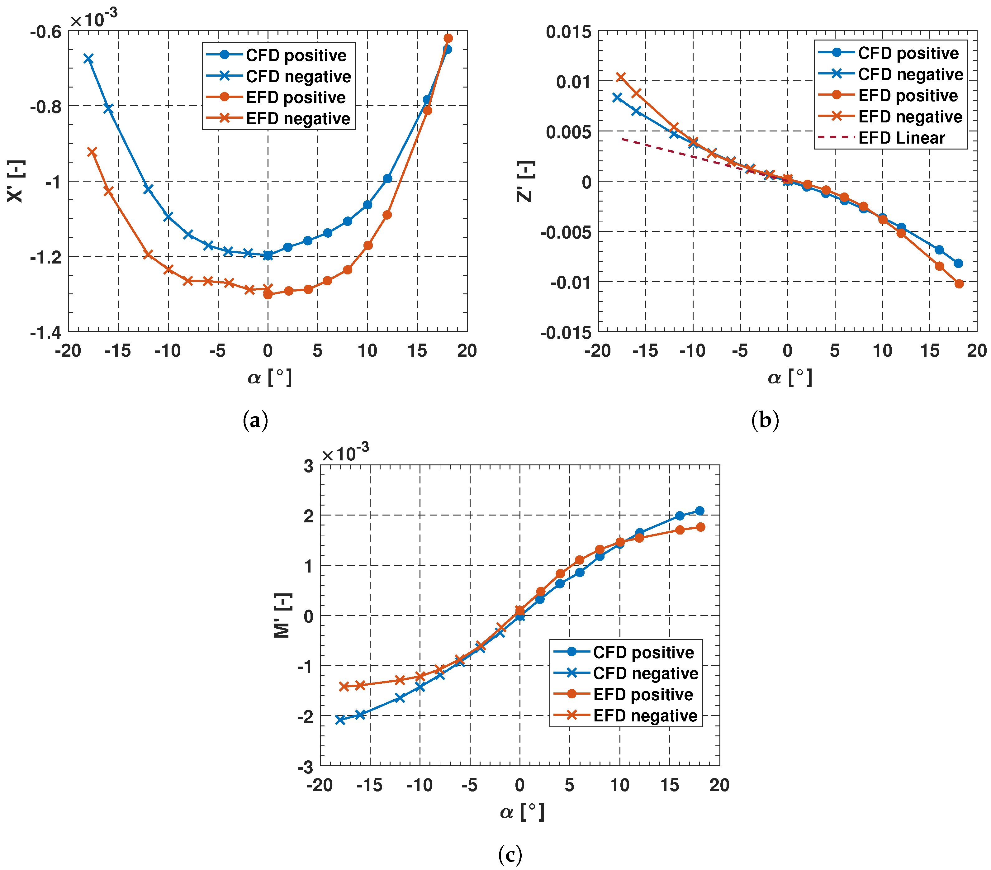
4.5. Fully Appended Configuration
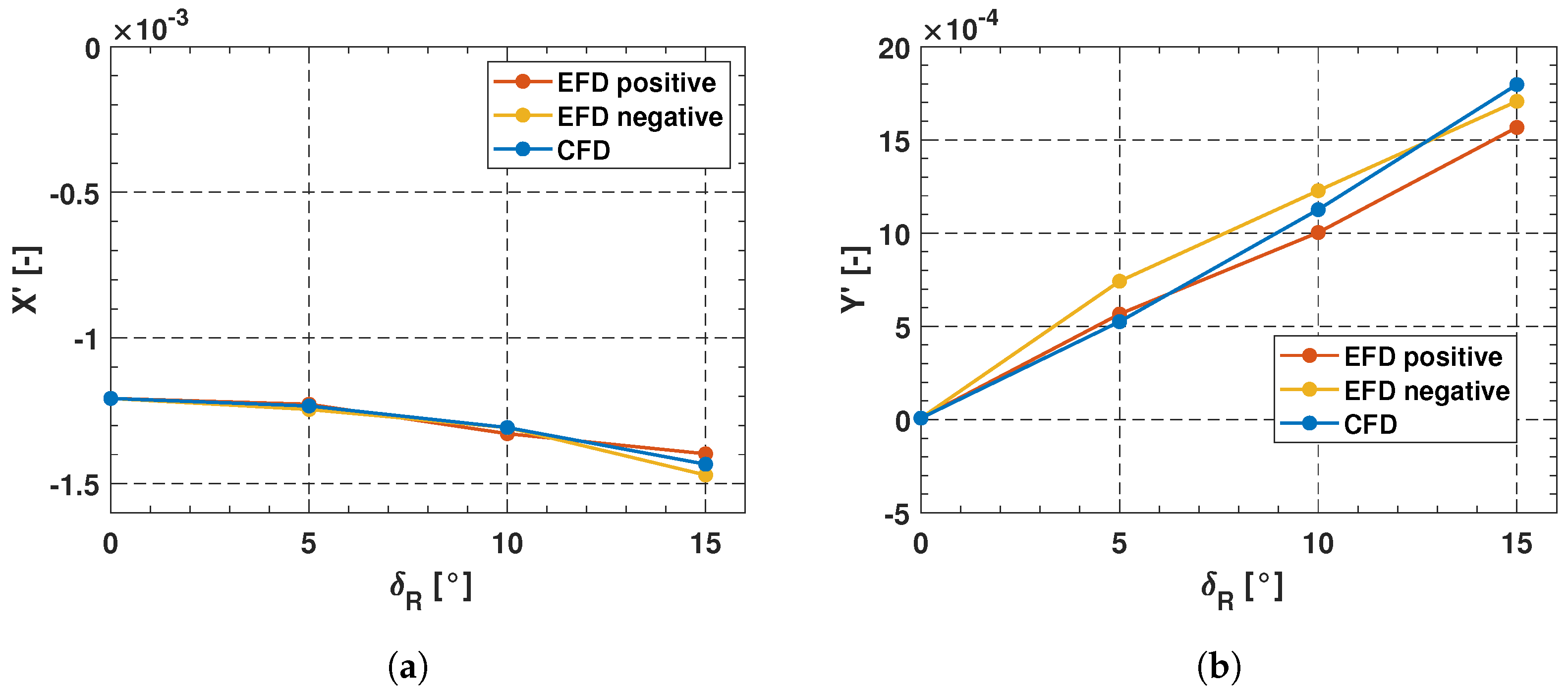
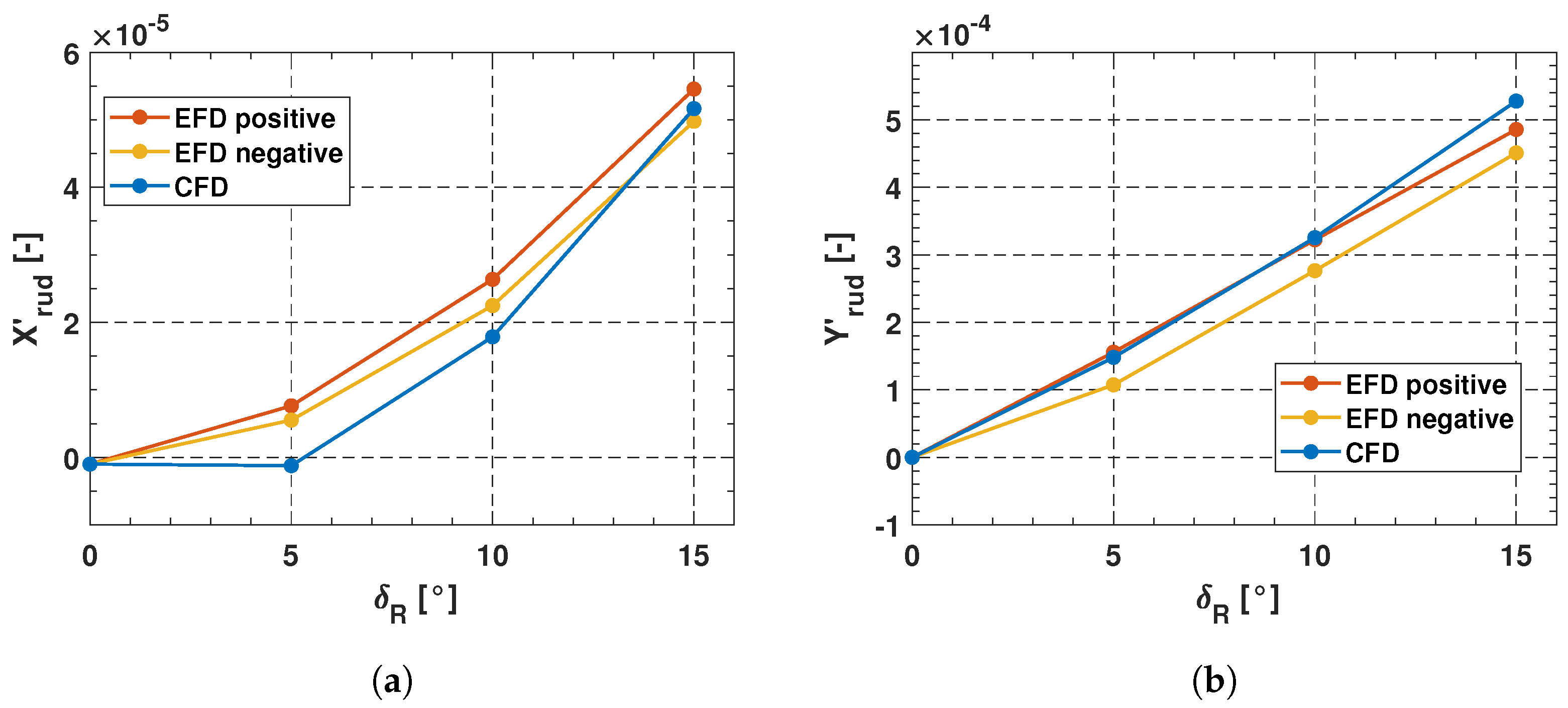
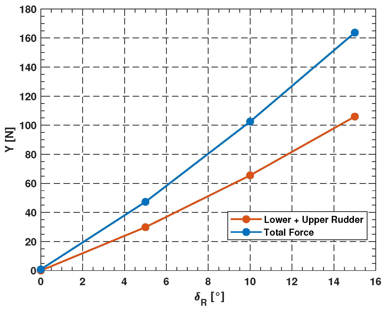
5. Results: Rudder Tests—Fully Appended Configuration
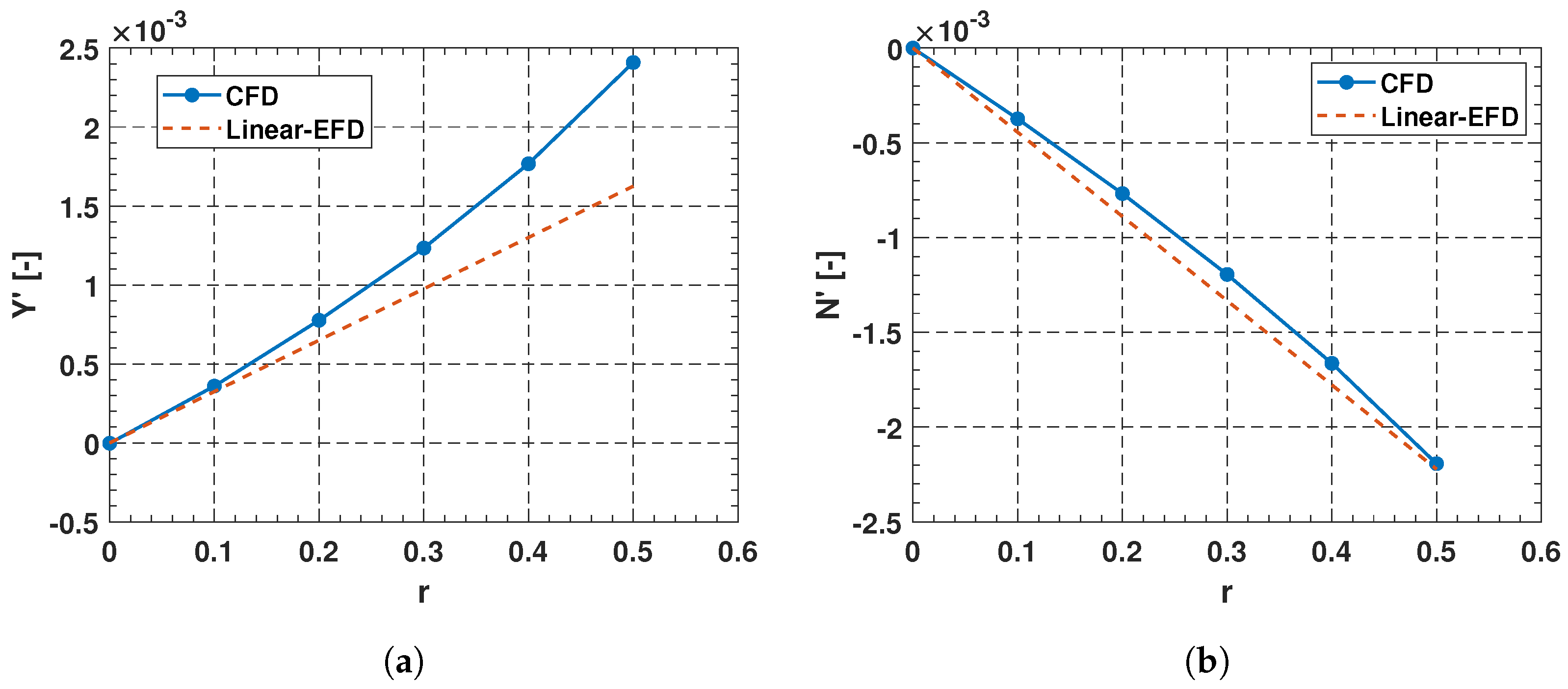
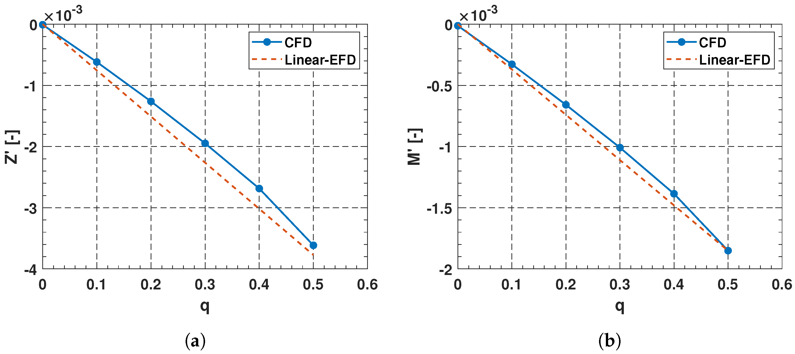
5.1. Results: Pure Rotation
6. Conclusions
Author Contributions
Funding
Institutional Review Board Statement
Informed Consent Statement
Data Availability Statement
Conflicts of Interest
References
- Lin, Y.H.; Tseng, S.H.; Chen, Y.H. The experimental study on maneuvering derivatives of a submerged body SUBOFF by implementing the Planar Motion Mechanism tests. Ocean Eng. 2018, 170, 120–135. [Google Scholar] [CrossRef]
- Renilson, M. Submarine Hydrodynamics; Springer: Berlin/Heidelberg, Germany, 2015; Volume 31. [Google Scholar]
- Hoyt, E.D.; Imlay, F.H.; David Taylor Model Basin Washington DC. The Influence of Metacentric Stability on the Dynamic Longitudinal Stability of a Submarine SRD 542/46 NS 512-001; David Taylor Model Basin Washington DC: Washington, DC, USA, 1948. [Google Scholar]
- Anderson, B.; Chapuis, M.; Erm, L.; Fureby, C.; Giacobello, M.; Henbest, S.; Jones, D.; Jones, M.; Kumar, C.; Liefvendahl, M.; et al. Experimental and computational investigation of a generic conventional submarine hull form. In Proceedings of the 29th Symposium on Naval Hydrodynamics, Gothenburg, Sweden, 26–31 August 2012. [Google Scholar]
- Quick, H.; Widjaja, R.; Anderson, B.; Woodyatt, B.; Snowden, A.D.; Lam, S. Phase I Experimental Testing of a Generic Submarine Model in the DSTO Low Speed Wind Tunnel; Client Report, DSTO-TN-1101; Defence Science and Technology Organisation: Victoria, Australia, 2012. [Google Scholar]
- Fureby, C.; Anderson, B.; Clarke, D.; Erm, L.; Henbest, S.; Giacobello, M.; Jones, D.; Nguyen, M.; Johansson, M.; Jones, M.; et al. Experimental and numerical study of a generic conventional submarine at 10 yaw. Ocean Eng. 2016, 116, 1–20. [Google Scholar] [CrossRef]
- Dubbioso, G.; Broglia, R.; Zaghi, S. CFD analysis of turning abilities of a submarine model. Ocean Eng. 2017, 129, 459–479. [Google Scholar] [CrossRef]
- Broglia, R.; Posa, A.; Bettle, M.C. Analysis of vortices shed by a notional submarine model in steady drift and pitch advancement. Ocean Eng. 2020, 218, 108236. [Google Scholar] [CrossRef]
- Lee, S.K.; Manovski, P.; Kumar, C. Wake of a cruciform appendage on a generic submarine at 10 yaw. J. Mar. Sci. Technol. 2020, 25, 787–799. [Google Scholar] [CrossRef]
- Wackers, J.; Deng, G.; Guilmineau, E.; Leroyer, A.; Queutey, P.; Visonneau, M. What is happening around the KVLCC2? In Proceedings of the 18th Numerical Towing Tank Symposium (NuTTS 2015), Cortona, Italy, 28–30 September 2015.
- Zhang, Z.; Guo, L.; Wei, P.; Wang, X.; Feng, D. Numerical simulation of submarine surfacing motion in regular waves. Iran. J. Sci. Technol. Trans. Mech. Eng. 2020, 44, 359–372. [Google Scholar] [CrossRef]
- Posa, A.; Balaras, E. A numerical investigation of the wake of an axisymmetric body with appendages. J. Fluid Mech. 2016, 792, 470–498. [Google Scholar] [CrossRef]
- Morse, N.; Mahesh, K. Large-eddy simulation and streamline coordinate analysis of flow over an axisymmetric hull. J. Fluid Mech. 2021, 926, A18. [Google Scholar] [CrossRef]
- Rocca, A.; Cianferra, M.; Broglia, R.; Armenio, V. Computational hydroacoustic analysis of the BB2 submarine using the advective Ffowcs Williams and Hawkings equation with wall-modeled LES. Appl. Ocean Res. 2022, 129, 103360. [Google Scholar] [CrossRef]
- Lungu, A. DES-based computation of the flow around the DARPA suboff. In Proceedings of the IOP Conference Series: Materials Science and Engineering, Kazimierz Dolny, Poland, 21–23 November 2019; Volume 591, p. 012053. [Google Scholar]
- Lungu, A. Large flow separations around a generic submarine in static drift motion resolved by various turbulence closure models. J. Mar. Sci. Eng. 2022, 10, 198. [Google Scholar] [CrossRef]
- Wang, L.; Martin, J.; Carrica, P.; Felli, M.; Falchi, M. Experiments and CFD for DARPA suboff appended with propeller E1658 operating near the surface. In Proceedings of the 6th International Symposium on Marine Propulsors, Rome, Italy, 26–30 May 2019; pp. 1–9. [Google Scholar]
- Wang, L.; Martin, J.E.; Felli, M.; Carrica, P.M. Experiments and CFD for the propeller wake of a generic submarine operating near the surface. Ocean Eng. 2020, 206, 107304. [Google Scholar] [CrossRef]
- Guo, H.; Li, G.; Du, L. Investigation on the flow around a submarine under the rudder deflection condition by using URANS and DDES methods. Appl. Ocean Res. 2023, 131, 103448. [Google Scholar] [CrossRef]
- Jones, D.A.; Clarke, D.B.; Brayshaw, I.B.; Barillon, J.L.; Anderson, B. The Calculation of Hydrodynamic Coefficients for Underwater Vehicles; Technical Report; Defense Technical Information Center: Fort Belvoir, VA, USA, 2002. [Google Scholar]
- Groves, N.C.; Huang, T.T.; Chang, M.S. Geometric Characteristics of DARPA Suboff Models: (DTRC Model Nos. 5470 and 5471); David Taylor Research Center: Bethesda, MD, USA, 1989. [Google Scholar]
- Roddy, R.F. Investigation of the Stability and Control Characteristics of Several Configurations of the DARPA SUBOFF Model (DTRC Model 5470) from Captive-Model Experiments; DTRC/SHD-1298-08; David Taylor Research Center, Ship Hydromechanics Department: Bethesda, MD, USA, 1990. [Google Scholar]
- Huang, T.T.; Liu, H.L.; Groves, N.C. Experiments of the Darpa (Defense Advanced Research Projects Agency) Suboff Program; David Taylor Research Center, Ship Hydromechanics Department: Bethesda, MD, USA, 1989. [Google Scholar]
- Joubert, P. Some Aspects of Submarine Design: Part 1: Hydrodynamics; Australian Department of Defence: Canberra, Australia, 2004. [Google Scholar]
- Joubert, P. Some Aspects of Submarine Design. Part 2. Shape of a Submarine 2026; Technical Report; Australian Department of Defence: Canberra, Australia, 2006. [Google Scholar]
- Overpelt, B.; Nienhuis, B.; Anderson, B. Free running manoeuvring model tests on a modern generic SSK class submarine (BB2). In Proceedings of the Pacific International Maritime Conference, Sydney, Australia, 6–8 October 2015; pp. 1–14. [Google Scholar]
- Du, P.; Cheng, L.; Tang, Z.j.; Ouahsine, A.; Hu, H.b.; Hoarau, Y. Ship maneuvering prediction based on virtual captive model test and system dynamics approaches. J. Hydrodyn. 2022, 34, 259–276. [Google Scholar] [CrossRef]
- Franceschi, A.; Piaggio, B.; Villa, D.; Viviani, M. Development and assessment of CFD methods to calculate propeller and hull impact on the rudder inflow for a twin-screw ship. Appl. Ocean Res. 2022, 125, 103227. [Google Scholar] [CrossRef]
- Franceschi, A.; Piaggio, B.; Tonelli, R.; Villa, D.; Viviani, M. Assessment of the Manoeuvrability Characteristics of a Twin Shaft Naval Vessel Using an Open-Source CFD Code. J. Mar. Sci. Eng. 2021, 9, 665. [Google Scholar] [CrossRef]
- Piaggio, B.; Villa, D.; Viviani, M. Numerical analysis of escort tug manoeuvrability characteristics. Appl. Ocean Res. 2020, 97, 102075. [Google Scholar] [CrossRef]
- Weller, H.G.; Tabor, G.; Jasak, H.; Fureby, C. A tensorial approach to computational continuum mechanics using object-oriented techniques. Comput. Phys. 1998, 12, 620–631. [Google Scholar] [CrossRef]
- Versteeg, H.K.; Malalasekera, W. An Introduction to Computational Fluid Dynamics: The Finite Volume Method; Pearson Education: Upper Saddle River, NJ, USA, 2007. [Google Scholar]
- Wilcox, D.C. Turbulence Modeling for CFD; DCW Industries: La Canada, CA, USA, 1998; Volume 2. [Google Scholar]
- Menter, F.R. Two-equation eddy-viscosity turbulence models for engineering applications. AIAA J. 1994, 32, 1598–1605. [Google Scholar] [CrossRef]
- Launder, B.E.; Spalding, D.B. Lectures in Mathematical Models of Turbulence; Academic Press: London, UK; New York, NY, USA, 1972; 169p. [Google Scholar]
- Spalding, D.B. The numerical computation of turbulent flow. Comp. Methods Appl. Mech. Eng. 1974, 3, 269. [Google Scholar]
- Shih, T.H.; Liou, W.W.; Shabbir, A.; Yang, Z.; Zhu, J. A new k-epsilon eddy viscosity model for high reynolds number turbulent flows. Comput. Fluids 1995, 24, 227–238. [Google Scholar] [CrossRef]
- Juretic, F. cfMesh User Guide; Creative Fields, Ltd.: London, UK, 2015; Volume 1. [Google Scholar]
- Zheku, V.; Villa, D.; Gaggero, S. A Detailed Analysis of Manoeuvring Performance of Solid of Revolutions. In Proceedings of the MARINE Conference, Madrid, Spain, 27–29 June 2023.
- Kim, H.; Leong, Z.Q.; Ranmuthugala, D.; Forrest, A. CFD modelling and validation of an AUV undergoing variable accelerations. In Proceedings of the ISOPE International Ocean and Polar Engineering Conference, Busan, Republic of Korea, 15–20 June 2014; p. ISOPE-I. [Google Scholar]
- Pan, Y.C.; Zhang, H.X.; Zhou, Q.D. Numerical prediction of submarine hydrodynamic coefficients using CFD simulation. J. Hydrodyn. 2012, 24, 840–847. [Google Scholar] [CrossRef]
- Amiri, M.M.; Esperança, P.T.; Vitola, M.A.; Sphaier, S.H. An initial evaluation of the free surface effect on the maneuverability of underwater vehicles. Ocean Eng. 2020, 196, 106851. [Google Scholar] [CrossRef]
- Amiri, M.M.; Esperança, P.T.; Vitola, M.A.; Sphaier, S.H. How does the free surface affect the hydrodynamics of a shallowly submerged submarine? Appl. Ocean Res. 2018, 76, 34–50. [Google Scholar] [CrossRef]
- Dawson, E. An Investigation into the Effects of Submergence Depth, Speed and Hull Length-to-Diameter Ratio on the near Surface Operation of Conventional Submarines. Ph.D. Thesis, University of Tasmania, Hobart, Australia, 2014. [Google Scholar]
- Celik, I.B.; Ghia, U.; Roache, P.J.; Freitas, C.J. Procedure for estimation and reporting of uncertainty due to discretization in CFD applications. J. Fluids Eng.-Trans. ASME 2008, 130. [Google Scholar] [CrossRef]
- Roache, P.J. Quantification of uncertainty in computational fluid dynamics. Annu. Rev. Fluid Mech. 1997, 29, 123–160. [Google Scholar] [CrossRef]
- Hoang, N.; Wetzel, T.; Simpson, R. Unsteady measurements over a 6: 1 prolate spheroid undergoing a pitch-up maneuver. In Proceedings of the 32nd Aerospace Sciences Meeting and Exhibit, Reno, NV, USA, 10–13 January 1994; p. 197. [Google Scholar]
- Kotapati-Apparao, R.B.; Squires, K.D. Prediction of a prolate spheroid undergoing a pitchup maneuver. In Proceedings of the 41 st AIAA Aerospace Sciences Meeting & Exhibit, Reno, NV, USA, 6–9 January 2003. [Google Scholar]
- Subrahmanya, M.; Rajani, B. Numerical Investigation of the Flow Past 6: 1 Prolate Spheroid. 2019. [Google Scholar]
- Chesnakas, C.J.; Simpson, R.L. Detailed investigation of the three-dimensional separation about a 6: 1 prolate spheroid. AIAA J. 1997, 35, 990–999. [Google Scholar] [CrossRef]
- Jeong, J.; Hussain, F. On the identification of a vortex. J. Fluid Mech. 1995, 285, 69–94. [Google Scholar] [CrossRef]
- Villa, D.; Gaggero, S.; Tani, G.; Viviani, M. Numerical and experimental comparison of ducted and non-ducted propellers. J. Mar. Sci. Eng. 2020, 8, 257. [Google Scholar] [CrossRef]
- Andersson, J.; Eslamdoost, A.; Vikström, M.; Bensow, R.E. Energy balance analysis of model-scale vessel with open and ducted propeller configuration. Ocean Eng. 2018, 167, 369–379. [Google Scholar] [CrossRef]
- Piaggio, B.; Vernengo, G.; Ferrando, M.; Mazzarello, G.; Viviani, M. Submarine Manoeuvrability Design: Traditional Cross-Plane vs. x-Plane Configurations in Intact and Degraded Conditions. J. Mar. Sci. Eng. 2022, 10, 2014. [Google Scholar] [CrossRef]
- Watt, G.; Gerber, A.; Holloway, A. Submarine hydrodynamics studies using computational fluid dynamics. In Proceedings of the CMHSC, Halifax, NS, Canada, 21–22 September 2007. [Google Scholar]
- Bettle, M.C. Baseline Predictions of BB2 Submarine Hydrodynamics for the NATO AVT-301 Collaborative Exercise; Defence Research and Development Canada: Toronto, ON, Canada, 2018. [Google Scholar]
- Pattison, D. Stability and Control of Submarines: A Review of Design Criteria and Derivative Prediction Techniques; Admiralty Experiment Works-Haslar: Gosport, South Hampshire, 1975. [Google Scholar]
- Pitts, W.C.; Nielsen, J.N.; Kaattari, G.E. Lift and Center of Pressure of Wing-Body-Tail Combinations at Subsonic, Transonic, and Supersonic Speeds; Technical Report; US Government Printing Office: Washington, DC, USA, 1957.


| Terms | Scheme |
|---|---|
| Convective term | Bounded Gauss LinearUpWindV (U) |
| Bounded Gauss upwind (k, , R, ) | |
| Diffusive term | Bounded Gauss upwind (k, , R, ) |
| Time integration | SteadyState |
| Laplacian term | Gauss linear limited 0.3 |
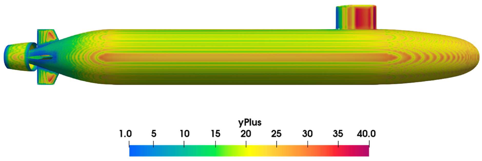
| Component | Requested | Obtained |
|---|---|---|
| Hull | 50 | 38.42 |
| Ring Wing | 50 | 48.37 |
| Sail | 50 | 48.37 |
| Upper Rudder | 50 | 44.74 |
| Lower Rudder | 50 | 44.74 |
| STB Sternplane | 50 | 44.74 |
| PS Sternplane | 50 | 44.74 |
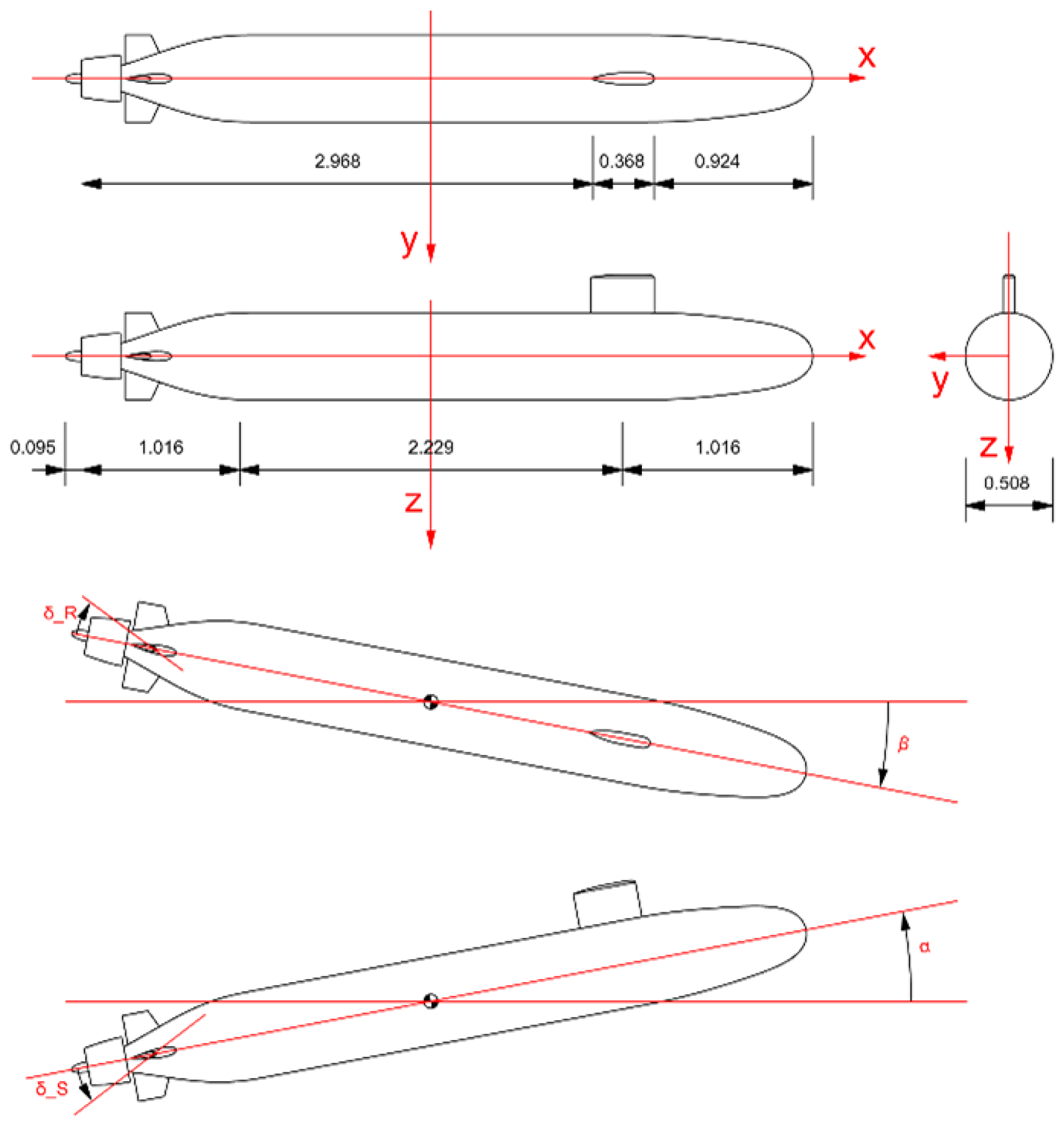
| Condition | Configuration | [] | [] | or [] |
|---|---|---|---|---|
| Pure drift (Horizontal) | // // | 0/+18 | 0 | 0 |
| Pure drift (Vertical) | 0 | −18/+18 | 0 | |
| Rudder Tests | 0 | 0 | +5/+15 | |
| Combined Tests (Horizontal plane) | 0/+18 | 0 | +5/+15 | |
| Combined Tests (Vertical plane) | 0 | −18/+18 | +5/+15 |
| Configurations | GCI |
|---|---|
| BH | 0.40% |
| BHSTAP | 1.64% |
| FA | 3.21% |
| Configurations | GCI |
|---|---|
| BH | 0.45% |
| BHSTAP | 1.82% |
| FA | 2.78% |
| DTRC | 4.49 | 8.86 | 73.55 | 9.96 | 13.85 | 29.86 |
| kOmega | 4.55 | 7.94 | 53.64 | 9.57 | 14.03 | 34.77 |
| kOmegaSST | 4.27 | 7.29 | 47.79 | 9.73 | 14.34 | 35.27 |
| kEpsilon | 4.63 | 8.00 | 59.66 | 9.52 | 13.97 | 33.46 |
| realizable kEpsilon | 3.97 | 8.77 | 61.39 | 9.66 | 13.70 | 32.64 |
Disclaimer/Publisher’s Note: The statements, opinions and data contained in all publications are solely those of the individual author(s) and contributor(s) and not of MDPI and/or the editor(s). MDPI and/or the editor(s) disclaim responsibility for any injury to people or property resulting from any ideas, methods, instructions or products referred to in the content. |
© 2023 by the authors. Licensee MDPI, Basel, Switzerland. This article is an open access article distributed under the terms and conditions of the Creative Commons Attribution (CC BY) license (https://creativecommons.org/licenses/by/4.0/).
Share and Cite
Zheku, V.V.; Villa, D.; Piaggio, B.; Gaggero, S.; Viviani, M. Assessment of Numerical Captive Model Tests for Underwater Vehicles: The DARPA SUB-OFF Test Case. J. Mar. Sci. Eng. 2023, 11, 2325. https://doi.org/10.3390/jmse11122325
Zheku VV, Villa D, Piaggio B, Gaggero S, Viviani M. Assessment of Numerical Captive Model Tests for Underwater Vehicles: The DARPA SUB-OFF Test Case. Journal of Marine Science and Engineering. 2023; 11(12):2325. https://doi.org/10.3390/jmse11122325
Chicago/Turabian StyleZheku, Vito Vasilis, Diego Villa, Benedetto Piaggio, Stefano Gaggero, and Michele Viviani. 2023. "Assessment of Numerical Captive Model Tests for Underwater Vehicles: The DARPA SUB-OFF Test Case" Journal of Marine Science and Engineering 11, no. 12: 2325. https://doi.org/10.3390/jmse11122325