Article

Effects of Leading-Edge Tubercles on Three-Dimensional Flapping Foils

1
School of Marine Science and Technology, Northwestern Polytechnical University, Xi’an 710072, China
2
State Key Laboratory of Digital Manufacturing Equipment and Technology, School of Mechanical Science and Engineering, Huazhong University of Science and Technology, Wuhan 430074, China
3
Xi’an Precision Machinery Research Institute, Xi’an 710072, China
*
Author to whom correspondence should be addressed.
J. Mar. Sci. Eng. 2023, 11(10), 1882; https://doi.org/10.3390/jmse11101882
Submission received: 10 August 2023 / Revised: 25 September 2023 / Accepted: 25 September 2023 / Published: 27 September 2023
(This article belongs to the Special Issue CFD Applications in Ship and Offshore Hydrodynamics)

Abstract

:
Recently, inspired by the flippers of humpback whales, researchers have been widely studying leading-edge tubercles for use as passive flow control devices. In this research, we numerically investigated the effects of leading-edge tubercles on a three-dimensional flapping foil coupled with rolling and pitching motions. Appropriate spanwise flexibility is considered to mimic the real flapping motion of humpback whales, and the profile of the angle of attack was analyzed in a representative section under the effects of spanwise flexibility. The motion of flexible foils was decomposed into rigid motion and flexible deflection by using the sliding mesh and dynamic mesh methods, respectively. Then, the hydrodynamic performance of the flexible flapping foils was estimated by solving the unsteady Reynolds Averaged Navier–Stokes equations. The effects of the shape and kinematic parameters on thrust, power consumption, and propulsive efficiency were studied and the mechanism behind these effects was investigated. A maximum efficiency loss of 19.4% was observed for the sharpest tubercle shape. Although the hydrodynamic advantages of leading-edge tubercles were not observed in the present study, the tendency of flow separation over peaking sections was suppressed under low angles of attacks. The results suggest that leading-edge tubercles are more suitable for foils with steady or quasi-steady motions, such as propellers or turbines.

1. Introduction

Owing to millions of years of evolution, aquatic animals demonstrate optimum hydrodynamic performance in terms of morphology and behavior. Therefore, they provide the best bionic inspiration for designing marine vehicles. The humpback whale (Megaptera novaeangliae), one of the largest aquatic animals, has evolved and exhibited outstanding maneuverability despite its huge body. Its maneuverability is attributed to the leading-edge tubercles on its pectoral flippers [1]. Morphological details of the humpback whale flipper have been evaluated and recorded [2]. Since then, numerous researchers have been interested in studying this unique structure to improve the performance of foils and wings.
For static foils, experimental and numerical methods have been employed to evaluate the impact of leading-edge tubercles. Wind tunnel measurements [3] and water tunnel tests [4] have indicated that the addition of leading-edge tubercles to foils delays their stall angle and improves their performance in the post-stall region. A flow visualization experiment [5] indicated that the flow over the peak sections of the tubercles is critical in the post-stall performance. Furthermore, numerical analyses have shown that the flow separation is suppressed over the peak sections owing to the streamwise vortices induced by the leading-edge tubercles [6,7]. This variation in the separation pattern is related to the weakening of the suction peak over the peak sections [8]. Static foils or wings can take advantage of leading-edge tubercles to improve the performance of rudders, for example [9].
Previous research on the effects of leading-edge tubercles has principally focused on static foils. However, most aquatic animals, especially humpback whales, acquire optimal propulsion and maneuverability by flapping their pectoral and caudal foils. Flapping motions are divided into three configurations: pitching or heaving only, combined pitching and heaving motions, and coupled rolling and pitching motions [10]. The coupled rolling and pitching motions are closest to the real motion of the foils of aquatic animals, such as turtles and humpback whales. In addition, this motion has three-dimensional kinematics, and the other two motions can be considered simplifications of this motion [10,11,12]. Therefore, this study focuses on coupled rolling and pitching motions, which can reflect the real motion form. A rigid three-dimensional flapping foil with coupled rolling and pitching motions was studied experimentally. The reported thrust and efficiency contours prove the superiority of these flapping foils [13]. The propulsive performance and flow details of the motion have been studied using a numerical method [11]. Flexibility is another key characteristic of bionic flapping foils and has recently received considerable attention. Spanwise flexibility was found to yield a small increase in the thrust coefficient and a small decrease in the power input requirement, resulting in higher efficiency [14]. Flexibility is also beneficial for improving the power extraction efficiency of flapping tidal generators [15].
In most studies, flapping motions have been performed on conventional foils with smooth leading edges. For flapping foils with leading-edge tubercles, a flow visualization experiment indicated that both the positive and the negative spanwise flows were attenuated [16]. Force measurements indicated a deteriorated hydrodynamic performance in the presence of leading-edge tubercles [17]. Numerical analyses also showed that leading-edge tubercles are disadvantageous for flapping performance [1]. These experiments and numerical simulations focused only on the difference between foils with and without leading-edge tubercles and ignored the tubercle shape. The effect of shape on the performance of insect-like flapping wings was studied and similar results were observed [18]. However, the motion was simple and the Reynolds number was low (400), which was not suitable for engineering. In addition, the mechanism of the effect was not focused on. In this research, the performance of three-dimensional flapping foils with leading-edge tubercles that move in coupled rolling and pitching motions was evaluated for different tubercle shape parameters and kinematic parameters at the Reynolds number of 50,000. The effect of leading-edge tubercles on flapping foils and the corresponding mechanism were focused on. Additionally, flexibility was considered to mimic the real flapping motion of humpback whales. The purpose of this study was to gain a deeper understanding of, first, the effect of leading-edge tubercles, and second, the morphology and behavior of humpback whales. These are useful in the design of bionic underwater vehicles.
The remainder of this article is organized as follows. Section 2 provides the problem statement and theoretical analysis. The numerical method used in this study is also described. The results are presented and analyzed in Section 3. In Section 4, the mechanisms of leading-edge tubercles and their effects on flapping foils are discussed. Section 5 summarizes the observations of this study and provides suggestions for further research.

2. Materials and Methods

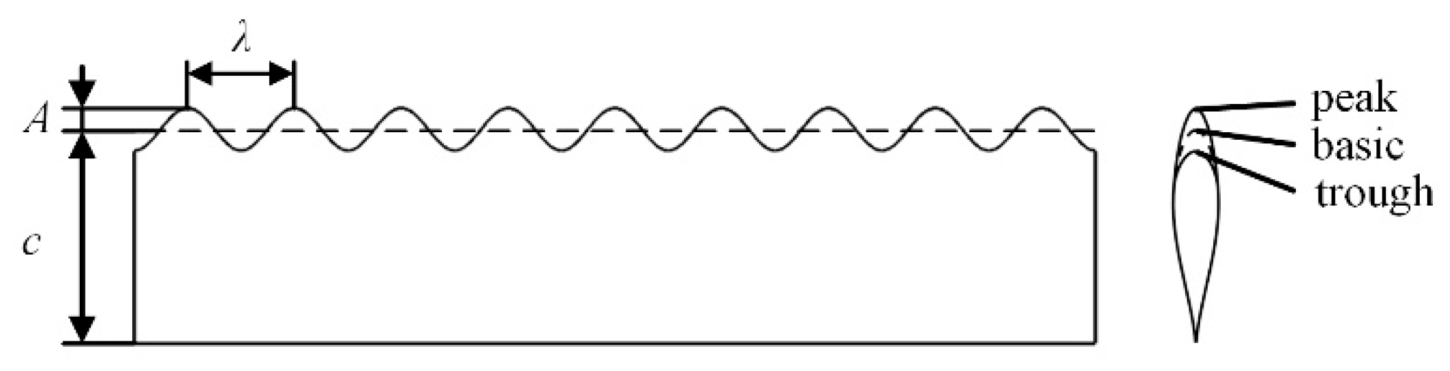
2.1. Description of Flapping Foils

A typical foil with leading-edge tubercles is shown in Figure 1. All modified foils were designed based on a rectangular foil with a smooth leading edge, chord length c = 100 mm, and span length b = 450 mm. The aspect ratio of a foil is defined as:
A R = b 2 S
where S is the planform area of the foil. The foils used in this study had an aspect ratio of 4.5, which is approximately equal to that of an idealized representation of a humpback whale flipper specimen [19].
The foils are based on the NACA 634-021 profile, which is similar to the cross-section of a humpback whale flipper [2]. The shape of the leading-edge tubercles for the modified foils is the same as that of a sinusoidal wave with amplitude A and wavelength λ in the spanwise direction. The cross-section of each modified foil was formed by first separating the head part from the basic profile and scaling its chordwise length and then reattaching it to the rest of the profile to maintain a smooth surface. A cross-section that is consistent with the basic profile exists between the peak and trough sections, where the chord length of the modified foils is defined.

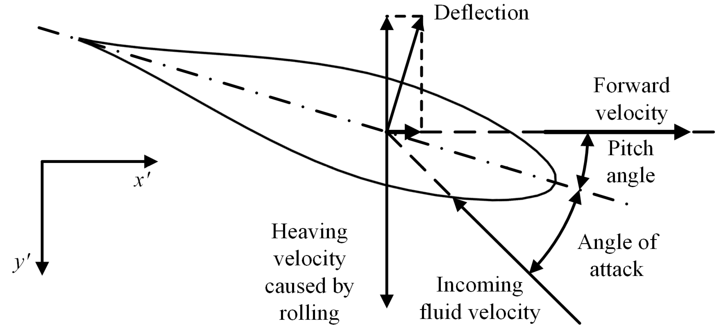
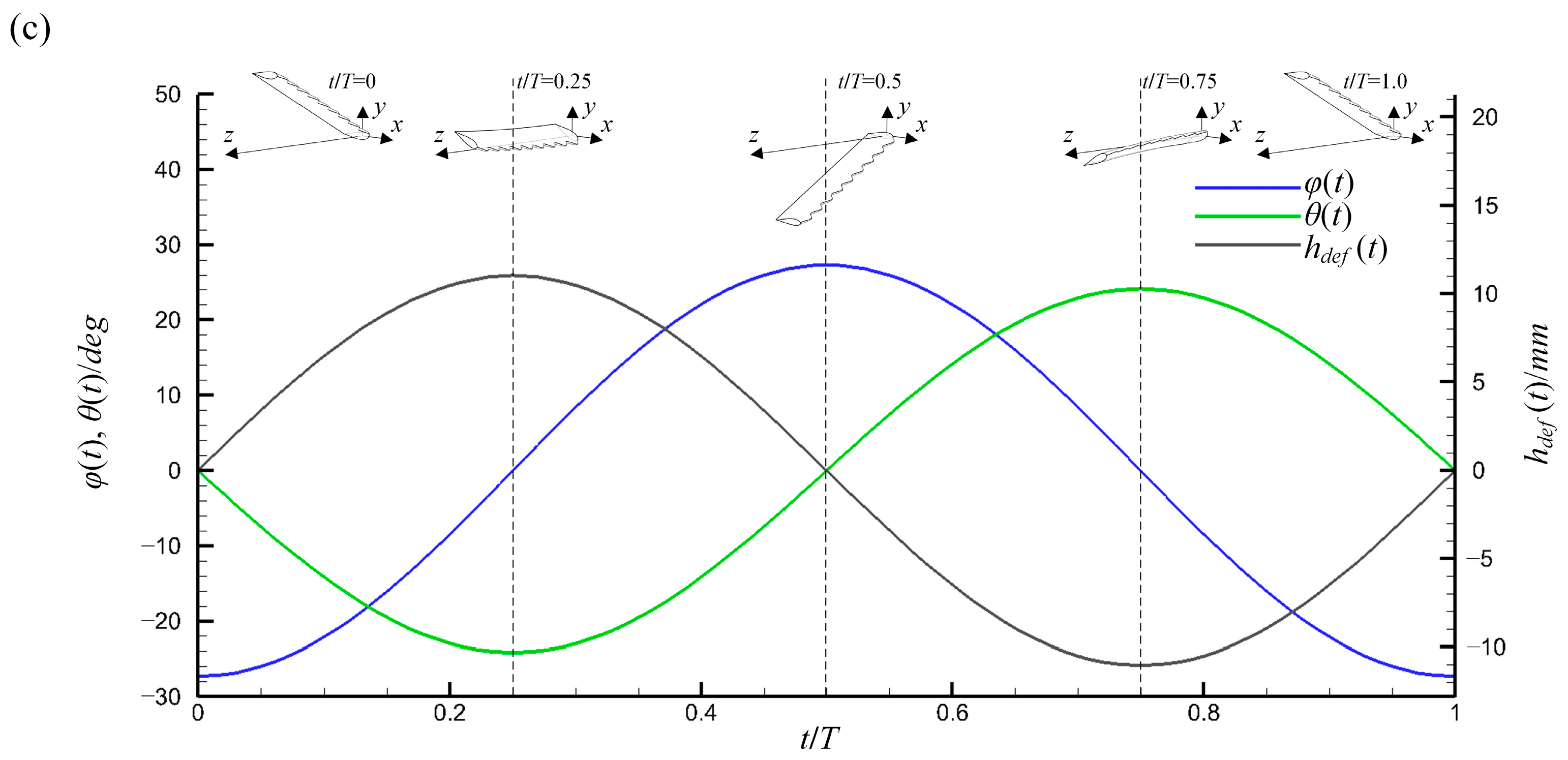
2.2. Kinematics Equations
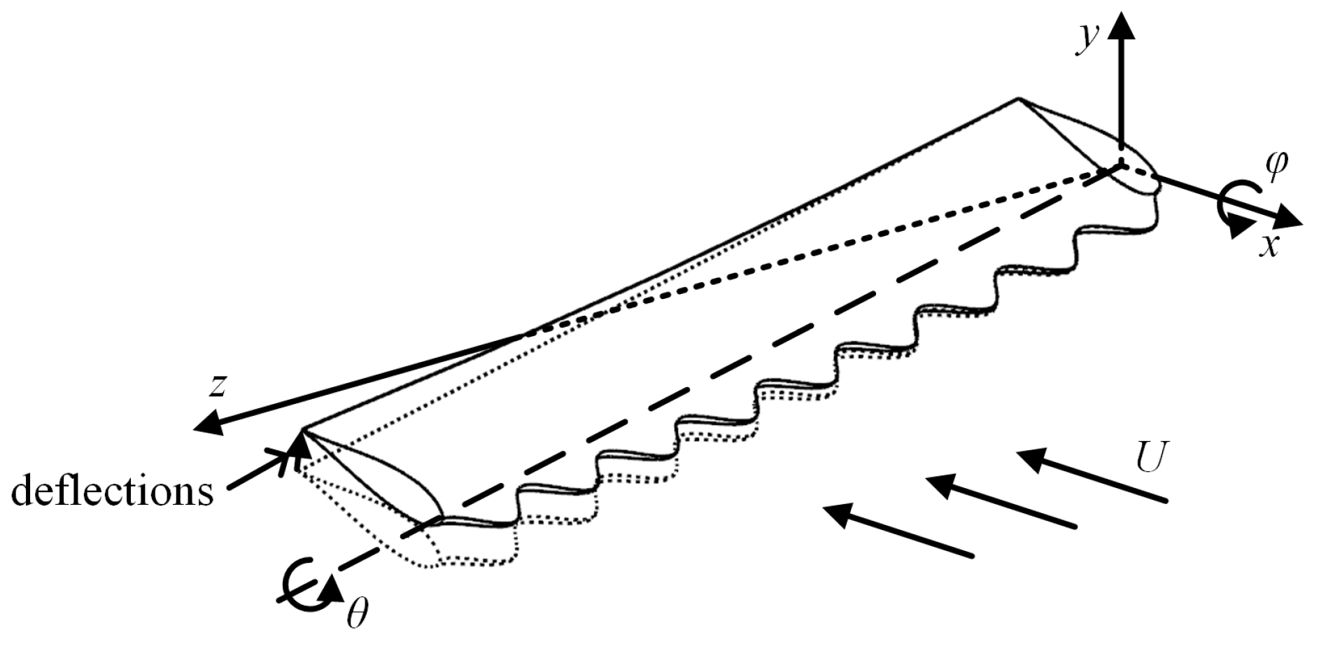
2.2.1. Rigid Motion

The flapping motion of foils with spanwise flexibility can be decomposed into rigid motion and flexible deflection, as shown in Figure 2. Rigid motion is composed of rolling and pitching motions, which are defined as:
φ ( t ) = φ 0 sin ( ω t )
θ ( t ) = θ 0 sin ( ω t - ψ p )
where φ ( t ) is the instantaneous rolling angle at which the foil rotates around the x -axis; θ ( t ) is the instantaneous pitching angle at which the foil rotates around the pitch axis, which is parallel to the trailing edge and located at distance of c/3 from the leading edge of the basic profile; φ 0 and θ 0 are the amplitudes of the rolling and pitching motions, respectively; ω is the circular frequency of the motion; and ψ p is the phase difference between the rolling and pitching motions, with its value set to π / 2 for optimal performance [20].

2.2.2. Spanwise Motion for Flexibility

During rigid motion, the spanwise flexibility is expressed as:
h d e f ( t ) = B ( s / b ) 2 sin ( ω t + ψ h )
where h d e f ( t ) is the spanwise deflection function, and B is the amplitude of deflection, with its value set to 0.05 b. Furthermore, s is the spanwise distance from the foil root, and ψ h is the phase difference between rolling and deflection, with its value set to π / 2 . The definition of spanwise flexibility is similar to that of a flapping tidal generator [15]. Moreover, as shown in Figure 2, the positive direction of deflection is defined as being perpendicular to the chord direction and at an acute angle to the y-axis.
The angle of attack varies along the span of the foils and depends on the rigid motion and flexible deflection at different span locations. The motion can be decomposed into 2D heaving and pitching motions at any spanwise location. To describe the kinematic parameters of this motion, a 70% span location was selected, which is a conventional position used in previous studies [13,17].
As shown in Figure 3, in the local velocity coordinates, the heaving motion at the selected location can be described as:
h ( t ) = h 0 sin ( ω t ) - h d e f ( t ) cos ( θ ( t ) )
where θ ( t ) = θ ( t ) is the pitch angle in the local coordinates, and h 0 is the amplitude of the heaving motion caused by the rolling motion, which is defined as:
h 0 = r 0.7 φ 0
where r 0.7 = 0.7 b is the spanwise distance between the selected location and the roll axis, and h 0 / c gives the amplitude of the rolling motion, which was set to 1.5, a value used by previous flapping foil experiments [13].
The instantaneous angle of attack is expressed as:
α ( t ) = arctan d ( h ( t ) ) / d t U + d ( h d e f ( t ) sin ( θ ( t ) ) ) / d t θ ( t )
where U is the forward velocity of the foils.
According to Equation (7), flexible deflection modifies the profile of α ( t ) . Figure 4 shows the variations in α ( t ) over one cycle for flexible and rigid foils when the maximum angle of attack ( α max ) is 20°. For rigid foils, by definition, B = 0 in Equation (4). For flexible foils, the moment at which the maximum angle of attack occurs lags behind that of the rigid counterparts. Meanwhile, the profiles on both sides of the extreme value become asymmetric.

2.2.3. Dimensionless Parameters
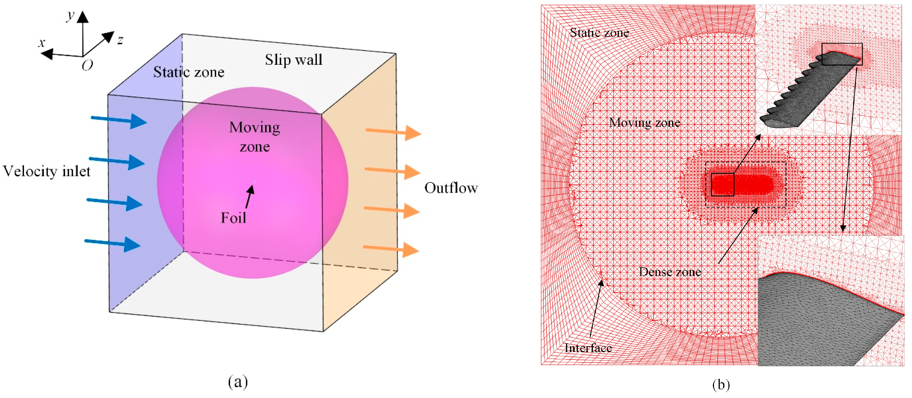
Two dimensionless parameters are defined to describe the kinematics of flapping foils. The Strouhal number (St), based on the heaving amplitude at the selected location, is defined as:
S t = 2 h 0 f U
where f is the motion frequency (Hz). At the limit position of the heaving motion, h d e f is zero, resulting in a heaving amplitude equal to h 0 .
The Reynolds number based on the chord length is defined as:
Re = U c ν
where ν 10 6 m 2 / s refers to the kinematic viscosity. A Reynolds number of 50,000 was considered in the present study.
The maximum angle of attack α max and the Strouhal number S t are defined as the free parameters. The amplitude of the pitching motion and the frequency can be calculated based on Equations (7) and (8) for a given α max and S t , respectively, which uniquely determine the motion.
We obtained the force and moment components on the foils along the x-, y-, and z-axes shown in Figure 2. The mean thrust F ¯ x and power consumption P ¯ are defined as:
F ¯ x = 1 T t t + T F x ( t ) d t
P ¯ = 1 T t t + T M r ( t ) φ ( t ) + M p ( t ) θ ( t ) d t
where T is the period of motion and F x is the x-component of instantaneous force. Moreover, M r ( t ) and M p ( t ) are the instantaneous moments in the rolling and pitching axes, respectively, and are expressed as:
M r ( t ) = M x ( t )
M p ( t ) = M y ( t ) sin ( φ ( t ) ) + M z ( t ) cos ( φ ( t ) )
where M x ( t ) , M y ( t ) , and M z ( t ) are the moments on the foil along the x-, y-, and z-axes, respectively. The minus sign denotes the output moment of the actuators.
The nondimensional mean thrust and power coefficients are denoted by C ¯ T and C ¯ P , respectively, and are defined as:
C ¯ T = F ¯ x 1 2 ρ U 2 S
C ¯ P = P ¯ 1 2 ρ U 3 S
where ρ is the density of water.
The instantaneous thrust and power coefficients, denoted by C T and C P , respectively, are defined in the same form as Equations (14) and (15), respectively, by replacing F ¯ x and P ¯ with F x and P , respectively.
The propulsive efficiency ( η ) of the foils is given by:
η = F ¯ x U P ¯ = C ¯ T C ¯ P

2.3. Approach

Most flapping foils used for propulsion operated in low-speed and underwater conditions. The ventilation and cavitation can be ignored, unlike the foils that cross free surface [21]. Thus, the flow around flapping foils is single-phase and incompressible. As previously described, both the geometry and motion studied in the present work are in three dimensions. Therefore, the three-dimensional single-phase incompressible unsteady Reynolds Averaged Navier–Stokes (RANS) equations were solved in the three-dimensional computational domain to study the flow over the foils. The governing equations are described as:
ρ u i x i = 0
ρ u i t + ρ ( u i u j ) x j = p x i + x j μ u i x j + u j x i + x j ( ρ u i u ¯ j )
where x i and x j ( i = 1 , 2 , 3 , j = 1 , 2 , 3 ) are the cartesian coordinate components. u i and u j are the velocity components and p is the pressure. μ = ρ ν is the dynamic viscosity. ρ u i u j ¯ is the Reynolds stress and needs to be solved by additional equations.
As shown in Figure 5a, the domain is divided into two zones: static and moving. The static zone is a cubic zone of 130   c × 130   c × 130   c , with an internal sphere space. A spherical zone of 110 c diameter was considered as the moving zone to achieve flapping motion of the flexible foils. Because the center of the moving zone coincides with the center of rotation of the foils, the rigid motion of the foils, which is described in Equations (2) and (3), can be achieved by rotating the zone around its center. During rotation, the interfaces of the two zones always coincide, making it possible to transmit flow information through the sliding mesh method. In addition, the dynamic mesh method is adopted in the moving zone to achieve spanwise deflection of the foils. The velocity inlet boundary condition was used in the upstream face of the cubic zone. The outflow boundary condition was used in the downstream face. The wall conditions were used in the other faces of the cubic zone and the foil surface. The shear stress of the wall of the cubic zone was set to 0 to ignore viscosity (called slip wall). The details of these boundary conditions can be found in Ref. [22]. The computational domain is discretized in space using a hexahedral grid for the static zone and a tetrahedral mesh for the moving zone, as shown in Figure 5b. A dense zone is defined in the wake region to accurately capture the flow details. A boundary layer mesh was generated by surrounding the surfaces of the foils to accurately obtain flow information near the foils.
The RANS equations were discretized in the computational mesh and solved using the finite-volume commercial code Fluent [23]. The SST  k ω turbulence model [24], developed for predicting flow with strong adverse pressure gradients and separation, was used to derive the Reynolds stress in the RANS equation. As an eddy viscosity-based model, the SST  k ω model has been widely used in industrial applications due to its simplicity and cost-effectiveness. However, the simplification made this model unsatisfactory under specific conditions. For instance, it proved challenging for this model to predict flows with significant effects of mean rotation and cases with non-inertial frames of reference. Concurrently, in turbulent flows where turbulent time scales were significantly smaller than the mean shear time scale, the model was likewise unsuitable [25]. The cases of the present study were outside these constraints. Even though the eddy viscosity assumption and the Reynolds-averaging process resulted in the loss of certain turbulence information, introducing uncertainty into the results [26], the hydrodynamic performance and main flow structures, which were the focus of the present study, could be effectively predicted by the RANS equations and the eddy viscosity-based model. This method has been widely employed in flapping foil simulations [27]. Moreover, the discretization errors associated with spatial and temporal terms, along with solution residuals, were additional sources of uncertainty. The numerical uncertainty was investigated in Section 2.4 using a grid-convergence study, considered the most common, straightforward, and reliable technique for the quantification of uncertainty [28].
In the present study, the pressure was discretized using a second-order scheme, and the momentum was discretized using a second-order upwind scheme. First-order upwind schemes were used for discretizing the turbulent kinetic energy and dissipation rate. The transient formulation is based on a first-order implicit scheme. The SIMPLEC algorithm was used to solve the pressure–velocity coupling equations. The zone motion specified with a user-defined function (UDF) was applied to the moving zone to achieve rigid motion while preserving the mesh quality. The flow information was transmitted between the two zones using a nonconformal sliding mesh interface. Moreover, the deflection of the foils was specified with UDF and was included in the simulations using the dynamic mesh method. The details of those numerical configurations are delineated in Ref [22]. All simulations were conducted for four cycles. In each time step, the convergence criterion of the pressure–velocity iteration was 0.0001 for the continuity. As shown in Figure 6, the residuals of all equations after solution convergence were less than 0.0001 at each time step. Meanwhile, we observed that the variations in forces and moments were periodic.

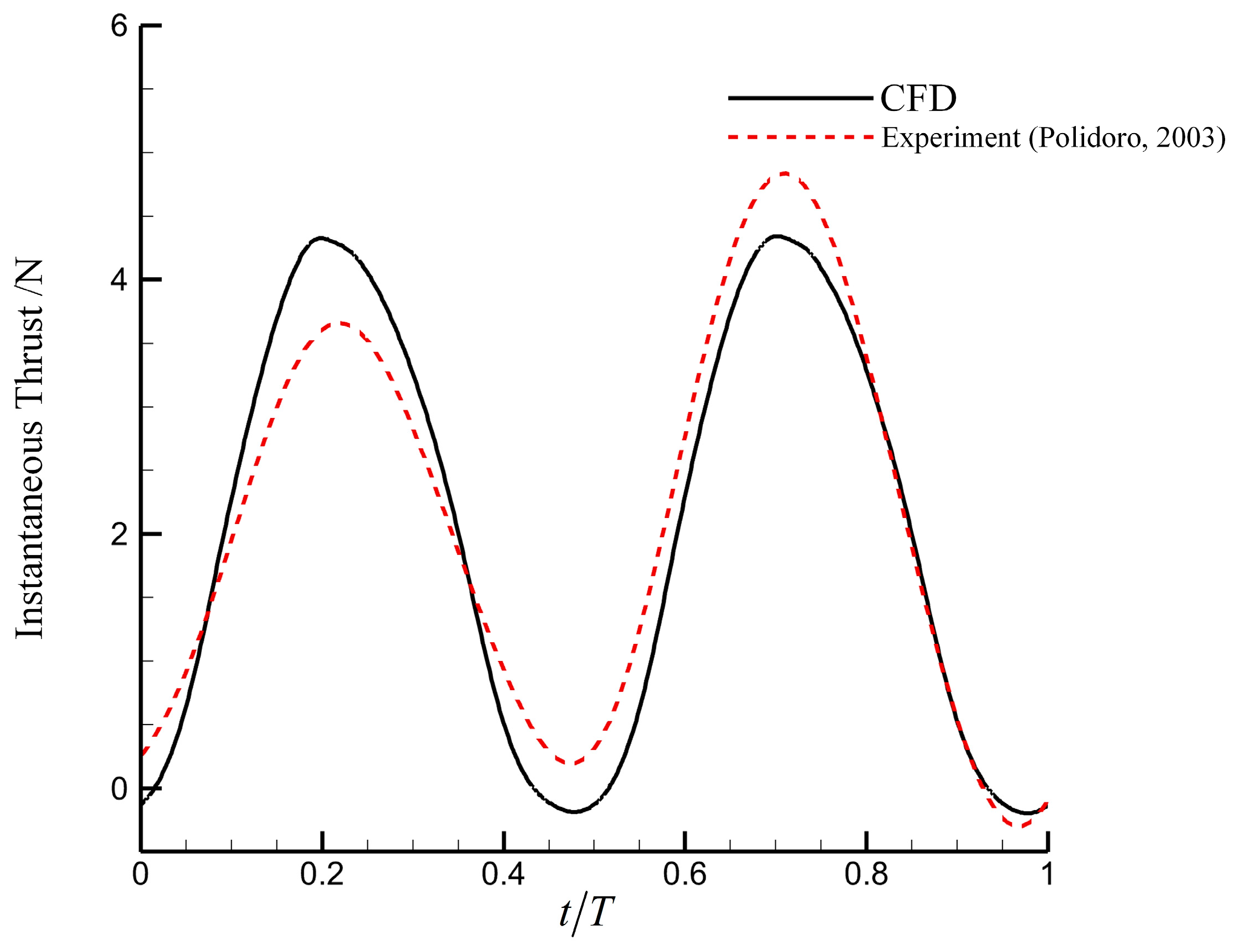
2.4. Validation and Verification

A flapping foil with a tubercle amplitude of 0.1 c and a wavelength of 0.25 c was considered for mesh and time validation. The motion parameters were St = 0.3 and α max = 20°. Three different values of mesh densities and time resolutions were considered, as discussed in this section. The details of different mesh densities and time steps and their mean thrust coefficients are listed in Table 1. For all configurations, the observed differences were less than 1%. As shown in Figure 7a, few differences in the instantaneous thrust coefficients were measured for each of the three mesh densities. Figure 7b shows a slice of the spanwise vorticity contours at the 70% span location for different mesh densities. The contours indicate that the flow could be accurately captured by the medium and fine meshes. Additionally, the standard grid-convergence index (GCI) method [29] was used to examine the uncertainty. The G C I f i n e 21 result, which describes the uncertainty between medium and fine meshes, was 0.13%. The accuracy of medium mesh is satisfied. Consequently, a medium mesh was used in the present work to balance the resource requirement and accuracy. The corresponding Y+ was less than 1 in most areas of the foil surface. Similarly, as shown in Figure 8, the time step size of T/500 was found to be the most economical and was selected for all simulations. The computational time for each case was approximately 86,400 s (24 h) at the selected mesh density and time step size (using two CPU AMD EPYC 7452 @ 2.35 GHZ (Cloud Computing Services Company, Beijing, China), 32 cores).
The verification of the method on 2D heaving and pitching flapping foils can be found in our previous work [30]. In the present study, the method was used on 3D NACA0012 foil with coupled rolling and pitching motions to verify the 3D applicability. The foil was a rectangular foil with chord length of c = 100 mm and a span length of b = 400 mm. This foil had a smooth leading edge and displayed a rigid flapping motion in the freestream with a Reynolds number of 50,000. The motion parameters were φ 0 = 60°, St = 0.4, and α max = 40°. The instantaneous thrust was obtained and compared with the experimental results [12]. As shown in Figure 9, the numerical results match well with the experimental data, indicating that the numerical method can effectively predict the hydrodynamic forces of flapping foils.

3. Results

Based on the representative range of amplitudes and wavelengths of tubercles found on humpback whale flippers [31], a total of four amplitudes and two wavelengths were considered in this study. A foil with a smooth leading edge was used for reference. The effects of St and α max were also investigated. The simulation parameters used in this study are listed in Table 2. The detailed parameters of Equations (2)–(4) under different motions are listed in Table 3. The time step sizes and corresponding Courant–Friedrichs–Lewy (CFL) numbers are also listed in Table 3. The CFL number is defined as C F L = Δ t U / Δ min , where Δ min is the minimum mesh length.

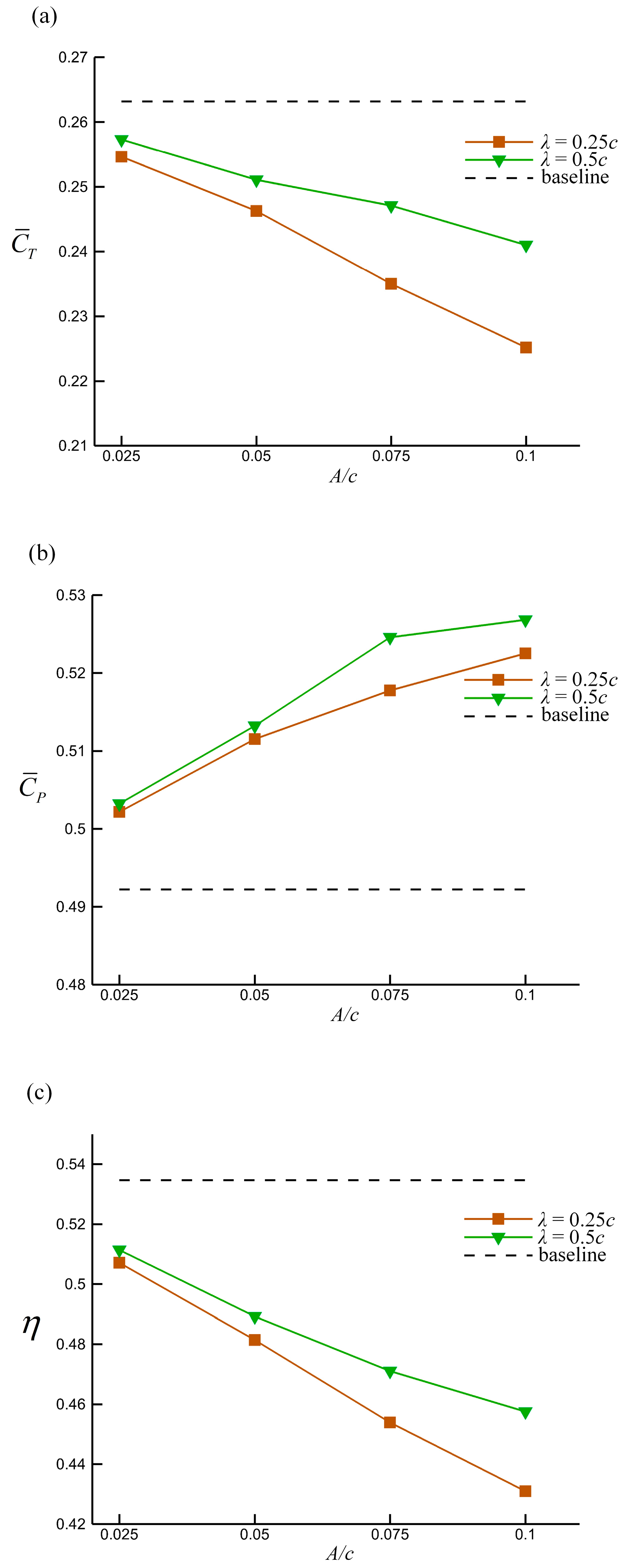
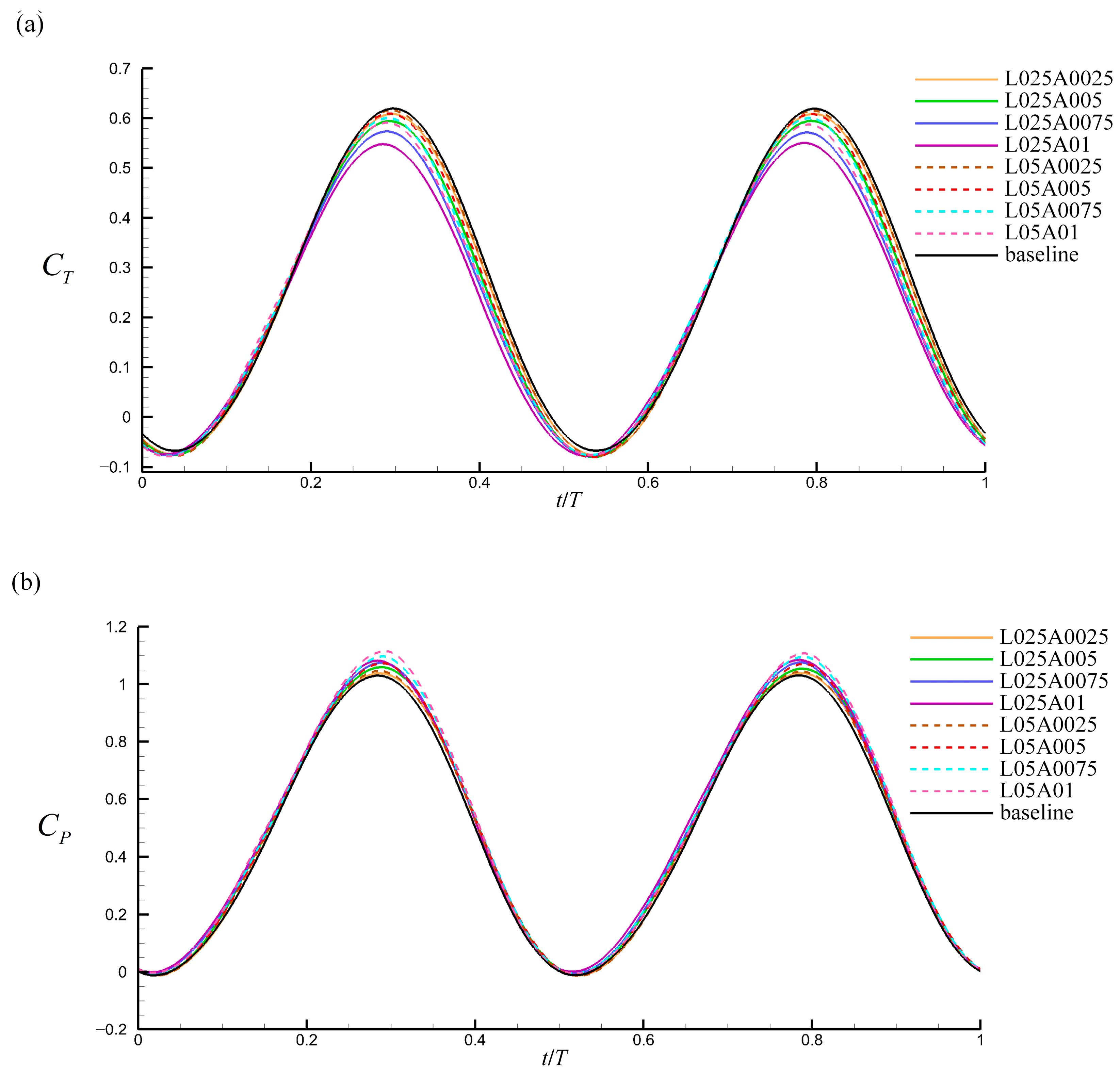
3.1. Effect of Tubercle Size

The performances of flapping foils with different tubercle sizes were investigated at St = 0.3 and α max = 20°, under which a high propulsive efficiency has been observed [13]. The mean thrust coefficients ( C ¯ T ), power coefficients ( C ¯ P ), and propulsive efficiency ( η ) were obtained and are shown in Figure 10. A decrease in thrust coefficients and an increment in power coefficients was observed under the effects of tubercles, thus reducing the propulsion efficiency. The tubercles exhibited a detrimental effect on the propulsive performance of the flapping foils within the range of wavelengths and amplitudes considered in this study. For both wavelengths, the loss of mean thrust increased approximately linearly with increasing amplitude. For a wavelength of 0.25 c, the maximum thrust loss was 14.4% at A = 0.1 c, whereas the average loss was 3.3% at A = 0.025 c. The power increment increased monotonically from 2% to 6.2% for a wavelength of 0.25 c and from 2.2% to 7% for a wavelength of 0.5 c. Compared with a wavelength of 0.25 c, a wavelength of 0.5 c produced more thrust and required more power. As the amplitude increased, the difference in thrust increased monotonically, reaching a maximum value of 7% at A = 0.1 c. However, the difference in power consumption initially increased till it reached a maximum of 1.3% at 0.075 c, after which it decreased. The results indicate that the effect of the leading-edge tubercles on the flapping foils increases sharply with amplitude, and that its effect on thrust is more significant. Therefore, the variation in the propulsive efficiency is similar to that of the thrust. Under the combined influence of thrust loss and power increment, a maximum efficiency loss of 19.4% was observed in the case of foil L025A01. In addition, because the effect of wavelength varies with the amplitude, it is difficult to consider these two parameters separately.
Figure 11 shows the instantaneous thrust coefficients ( C T ) and power coefficients ( C P ) for different foils over one cycle, as well as their corresponding positions. The thrust and power coefficients showed distinct periodicity with twice the frequency of the flapping motion. The moment at which the peaks of thrust and power consumption occurred lagged slightly behind the instant at which the foil was at the center of its trajectory; this is related to the angle-of-attack profile. A slight drag and power production were observed near where the roll motion was in the limit position. Under the effects of the leading-edge tubercles, the peak values of the thrust and power coefficients changed significantly. These values are listed in Table 4. The variation in the peak was similar to that of the mean coefficients, indicating that the peak variation is crucial in the hydrodynamic performance loss.
To further analyze the effects of the tubercles on the flow, foil L025A01, which had the most distinct effect, was selected. The slices of the spanwise vorticity contour of this foil when the thrust peak occurred are shown in Figure 12a. For reference, the corresponding baseline foil is shown in Figure 12b. The strength of the spanwise vorticity gradually increased along the foil span toward the tip direction. No significant flow separation was observed for either foil; however, a clear distinction was observed between the spanwise vorticities of the modified foil and the baseline. The spanwise vorticities of the modified foil were suppressed near the leading edge in the peak sections and strengthened in the trough sections. Specifically, the separation tendency was suppressed in the peak sections and strengthened in the trough sections, which was observed in static airfoils [4]. However, the suppression of separation led to different effects on the performance of static and flapping foils. A difference in flow behind the tubercle peaks and troughs has also been observed in a static wing with spanwise waviness [32].
The pressure distribution along the chordwise direction and in the direction perpendicular to it in the peak and trough sections, which are marked in Figure 12a near the 70% span location, are presented in Figure 13a,b. No significant difference was observed in the pressure distribution between these two locations for the baseline. Thus, only the pressure distribution at the location corresponding to the peak section is provided for reference. The pressure distribution of the modified foil differed significantly from that of the baseline in the peak and trough sections. The suction peak decreased in the peak section and increased in the trough section, which was related to the variation in the hydrodynamic force and flow around the foil.
Figure 14 shows the force diagram for a section and the distribution of the pressure vector on the sections corresponding to Figure 13. Under the action of pressure, a force Fc along the chord direction and a force Fpc along the direction perpendicular to it are generated on the section. The thrust and power of the foil can be described as:
T = 0 b F p c sin ( θ ) + F c cos ( θ ) d s
P = 0 b ( F p c cos ( θ ) F c sin ( θ ) ) h ( s , t ) + M s θ d s
where h ( s , t ) is the heaving velocity of the section, and Ms is the moment of the section around the pitch axis. Because the pitch angle approaches its maximum value when the thrust and power peaks occur, the M s θ is small and can be ignored. The variation in pressure distribution primarily occurs in the suction area near the leading edge of the upper portion, which is related to the chordwise force Fc. In the peak section, as shown in Figure 13a, the hydrodynamic force Fpc has no significant variation under the combined effect of the weakening of the suction peak and increased local chord length. However, the loss of the area enclosed by the pressure coefficient curve of the peak section shown in Figure 13b indicates that the reduction in the suction peak led to the loss of chordwise force Fc. According to Equations (19) and (20), thrust is reduced and power consumption is increased. In the trough section, the pressure distribution had no significant influence on the hydrodynamic performance, which is caused by variations in the suction peak and the local chord length.
In the peak section, high- and low-pressure regions were created in the lower and upper portions of the foil, respectively; these regions were induced by the angle of attack. The pressure difference drives the flow from the lower to the upper portion through the valleys of the tubercles, which is blocked in the baseline. Figure 15 shows the spanwise velocity contours in the middle section between the peak and trough sections, which are marked in Figure 12a. A positive velocity represents the flow moving from the peak to the trough. The results indicate that the flow moved towards the trough in the lower portion and towards the peak in the upper portion near the leading edge. This flow was similar to that near the tip of the wing and weakened the suction in the peak section, which led to a reduction in adverse pressure gradients. Positive pressure gradients were generated near the leading edge in the upper portion, which contributed to the suppression of the flow separation. Conversely, in the trough section, the suction peak increased under the effects of the flow induced by tubercles. The increase in the suction peak and the reduction in the local chord length resulted in higher adverse pressure gradients, which can strengthen the flow separation. Variations in the suction peak and flow were also observed by Serson et al. [8].

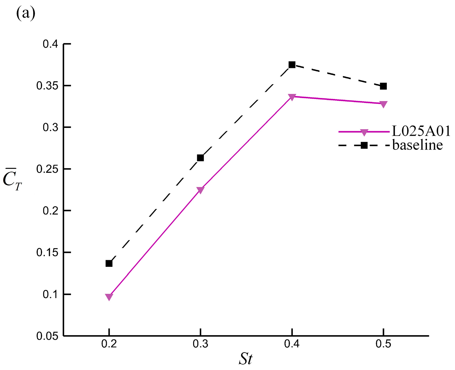
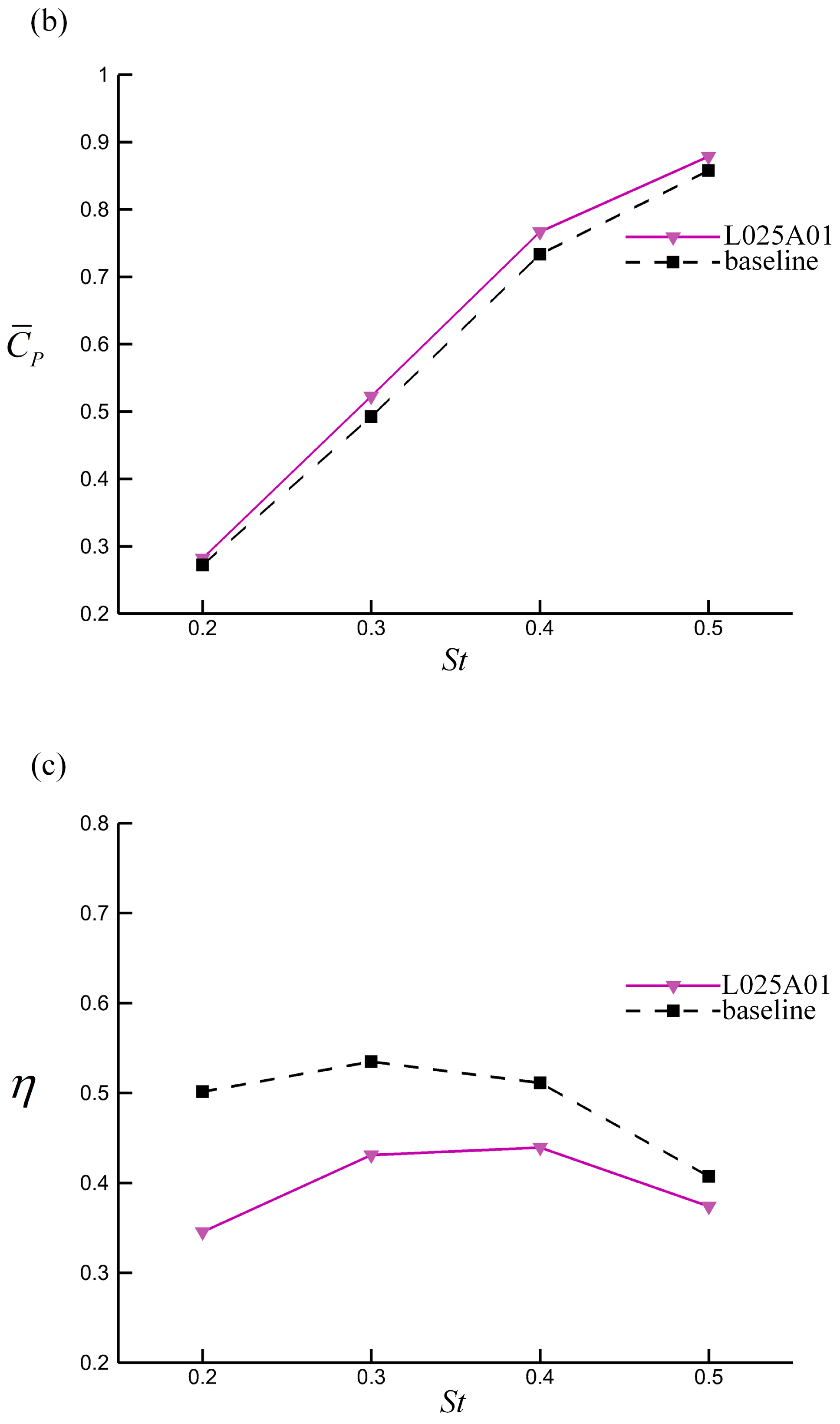
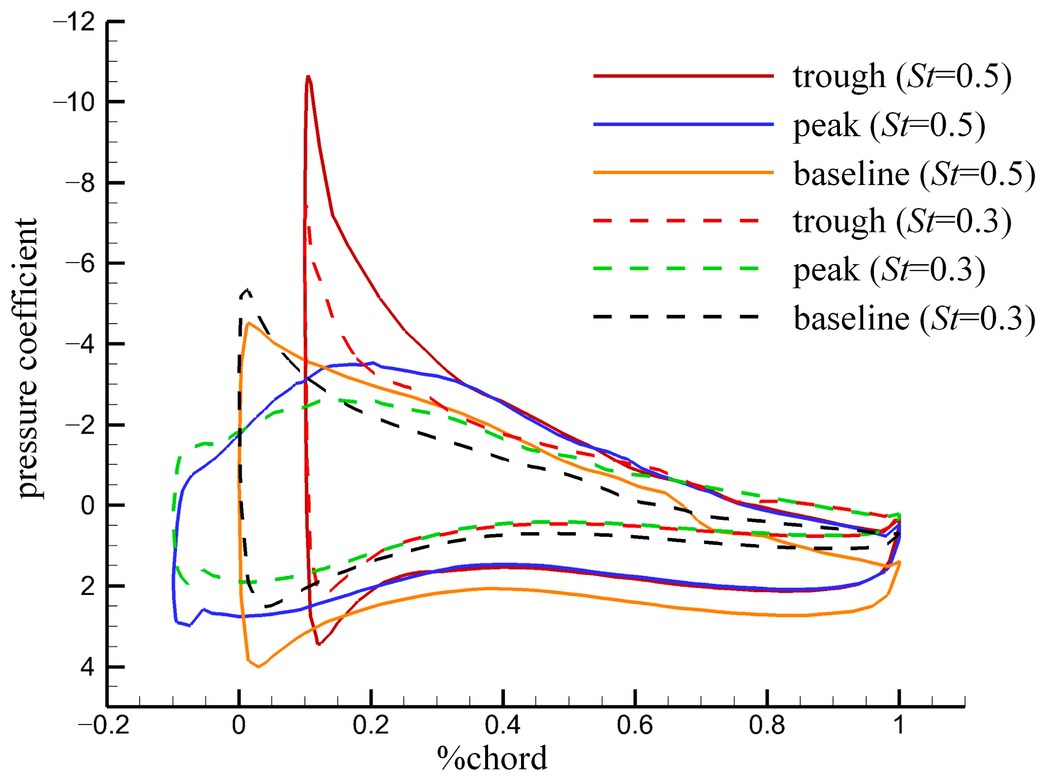
3.2. Effect of Strouhal Number

For a flapping foil, the Strouhal number is a kinematic parameter that significantly affects propulsive performance. As discussed in Section 3.1, foil L025A01, which had the most distinct effect, was considered in the St range of 0.2–0.5 at α max = 20°. The mean hydrodynamic performance is presented in Figure 16. The results indicate that the thrust increased approximately linearly in the St range of 0.2–0.4, after which it decreased. A monotonic increment was observed for power consumption over the entire St range considered in the present study; however, the rate of increase declined for St values above 0.4. As St increased, the propulsive efficiency, which depends on the thrust and power consumption, first increased and then decreased. For the modified foil, the maximum efficiency was observed for St = 0.4, whereas that of the baseline was at St = 0.3. Although a loss of propulsive performance was observed, the difference between the modified foil and baseline gradually decreased, indicating that the effect of tubercles changed from weakening to enhancement. However, an enhancement of the propulsive performance was not observed in the St range considered in this study.
We further investigated the effects of tubercles at different Strouhal numbers. Figure 17 shows the pressure distribution of the modified foil in the same sections as that in Section 3.1 at St = 0.5, when the foil had the maximum instantaneous thrust. The results of St = 0.3 are also presented as a reference. The pressure distribution pattern does not depict a significant difference between different Strouhal numbers, indicating that the flow was not drastically changed by the variation in Strouhal numbers. However, the pressure difference between the upper and lower portions of the foil increased at a high Strouhal number, indicating an increase in thrust and power consumption. In addition, we observed less weakening of the suction peak in the peak section and an increase in the suction peak in the trough section, which benefitted the propulsive performance. Compared with the suction at a low Strouhal number, that near the leading edge in the upper portion of the foil decreased in the peak section and increases in the trough section, indicating that the effects of the tubercles were enhanced at high Strouhal numbers. This variation in the pressure distribution indicates that the transition of effects decreases the difference between the modified foil and the baseline as the Strouhal number increases instead of suppressing these effects.

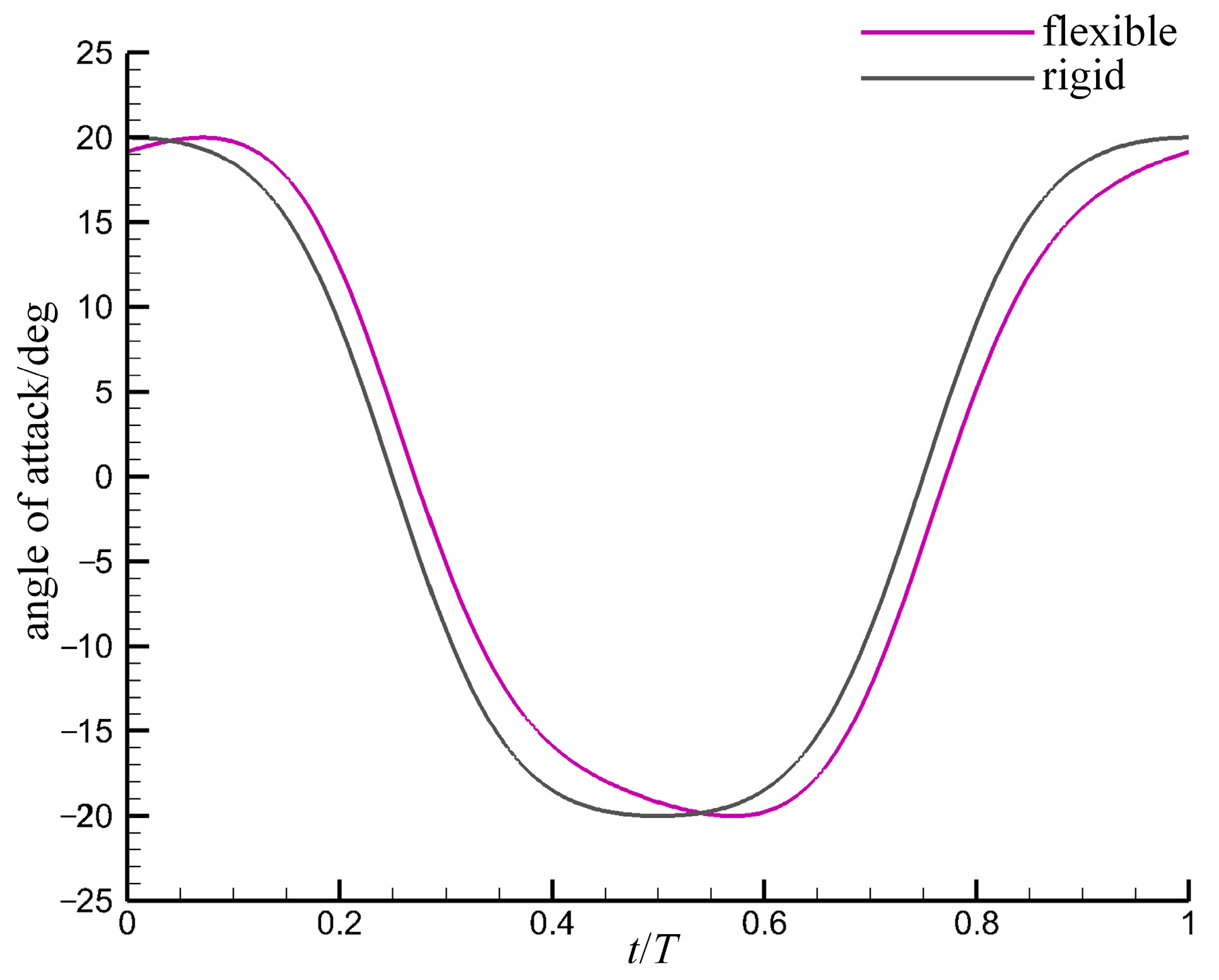
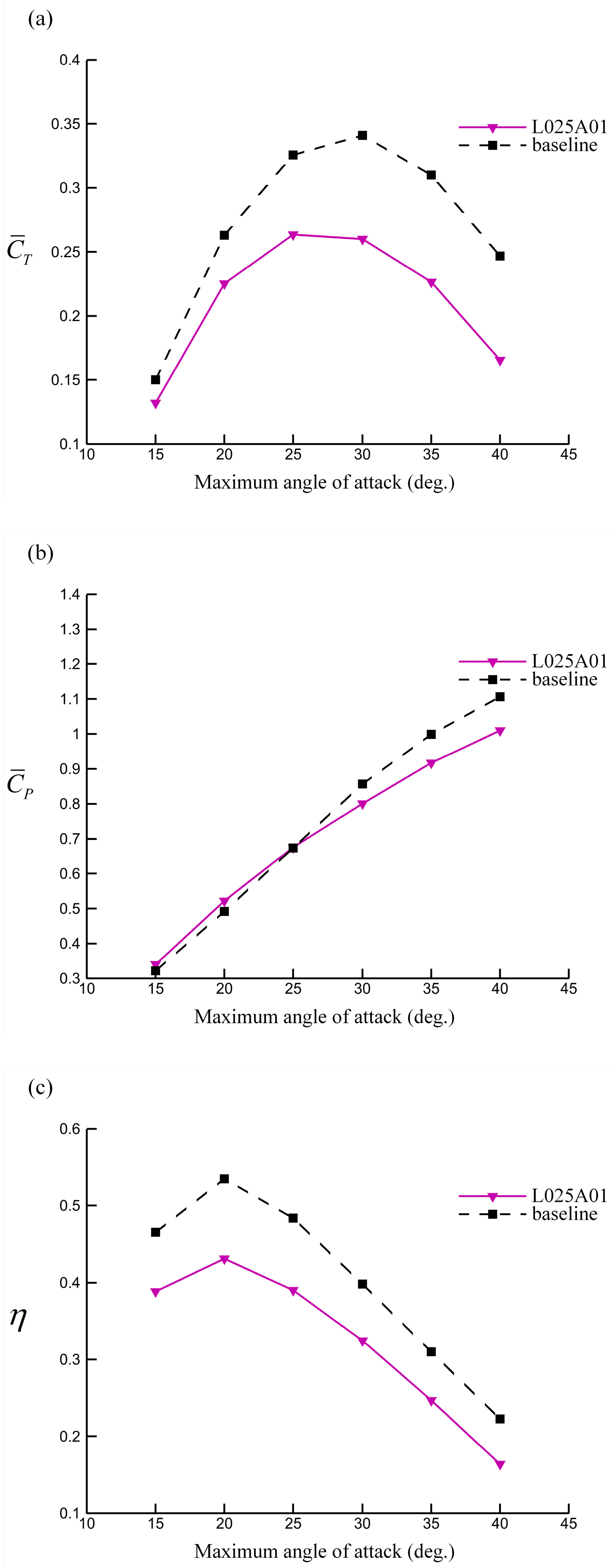
3.3. Effect of Maximum Angle of Attack

In addition to the Strouhal number, the maximum angle of attack ( α max ) plays a significant role in the flapping foil performance. The performance of foil L025A01 was considered in the α max range of 15–40° at St = 0.3. The mean propulsive performance is plotted in Figure 18. With the increment in α max , the mean thrust first increased and reached a peak at α max = 25° for the modified foil and at α max = 30° for the baseline. Then, as α max was increased further, the thrust decreased. The power consumption increased over the entire range of α max , as shown in Figure 18b. The propulsive efficiency first increased till it reached a maximum at α max = 20°, after which it decreased. Variation in the effects of the tubercles was observed at different values. A loss of thrust existed in the entire considered range of α max and increased with the increment in α max . The power consumption of the modified foil was greater than that of the baseline in the range of α max 25 ° and lesser than that for α max > 25°. Although the reduction in power consumption was greater at high values, the propulsive efficiency of the modified foil was less than that of the baseline owing to the greater loss of thrust. These results indicate that tubercles cannot benefit the propulsive performance of the flapping foils, even at high values.
Figure 19 shows the pressure distribution in the same peak and trough sections at α max = 40°, which is when the foil had the maximum instantaneous thrust. The pressure distribution on the upper portion of the modified foil varied greatly at a high α max . Multiple suction peaks appeared in the peak and trough sections, indicating that the flow became more complex in these two sections under the effects of a high α max . The maximum suction peaks in these sections were reduced compared with that of the baseline, inducing a loss of thrust and reduction in power consumption. The hydrodynamic performance in the peak and trough sections was weakened, which is different from the low α max . Slices of the spanwise vorticity contour for the modified foil and baseline at α max = 40° are presented in Figure 20. The flow of the baseline foil separated from the leading edge in the outer region with approximately a quarter of the span length and reattached to the upper portion of the foil at the half-chord position. However, the presence of tubercles expanded the separation region and strengthened the flow separation in the peak and trough sections. Only the flow separation near the leading edge on the upper portion of the tubercles in the peak sections was suppressed. The strengthening of the separation led to a reduction in the maximum suction on the upper portion, thus weakening the hydrodynamic performance.

4. Discussion

In contrast to static foil behavior, flapping foils do not take advantage of tubercles. A reduction in the propulsive performance was observed for all modified foils in the considered range of kinematic parameters. For the leading-edge tubercles, suppression of flow separation was observed in the peak sections. However, no significant flow separation occurred on the foil surface. Hence, it was difficult for the tubercles to work. Furthermore, the presence of tubercles strengthened the separation tendency and expanded the separation regions. The variation in the flow changed the pressure distribution on the foil surface, thus diminishing the propulsive performance of the modified foils.
For static foils, the streamwise vortices generated by the tubercles play a pivotal role in delaying stall [33]. The vortices can inject high-momentum fluid into the boundary layer behind the peak sections, thus delaying flow separation [7]. Similar streamwise vortices were also generated for the flapping foils, as shown in Figure 21. However, a similar flow yielded different results. Earlier force measurements showed that the foils with tubercles produced less thrust while consuming the same amount of power. This phenomenon was hypothesized to stem from the breakdown of the thrust wake due to the interaction between the streamwise vortices and those generated by flapping [17]. In the present study, foils with tubercles generated less thrust and consumed more power, except in high angles of attack. Such variances might be attributed to foil tapering. Furthermore, this study interpreted the performance deterioration from a distinct perspective. The vortices generated by the tubercles diminished the suction peak in the peak sections, resulting in a decrease in the chordwise forces and ultimately inducing performance deterioration. However, the interrelationship between the variation in pressure distribution and the thrust wake requires further investigation. On the other hand, the vortices suppressed the flow separation on the tubercle surface in the peak sections, whereas they strengthened the separation in the remaining regions after interacting with the flow of the flapping foil. Moreover, for flapping foils, it is difficult to maintain the instantaneous angles of attack at relatively high values for a long time. Consequently, the flow cannot be fully developed, and the flow separation is suppressed by the motion. However, the presence of streamwise vortices strengthens the flow separation in the trough regions. Therefore, the presence of leading-edge tubercles was found to be disadvantageous.
Considering these effects of tubercles on the flapping foils, leading-edge tubercles can be considered unsuitable for use in general flapping foils. It makes sense that the tubercles have not evolved in animals that drive themselves by flapping their foils or wings, such as turtles and birds. They are more suitable for foils that move with steady or quasi-steady motions, such as the flippers of humpback whales in nature, and in propellers or turbines used in ocean engineering, where performance improvement has been observed [34,35].

5. Conclusions

In this research, we investigated the effects of leading-edge tubercles on a three-dimensional flexible flapping foil at different Strouhal numbers and maximum angles of attack. The performance of flapping foil was estimated using verified numerical methods. The effects of leading-edge tubercles with different amplitudes and wavelengths were estimated under conditions of high propulsive efficiency. Leading-edge tubercles caused a loss of thrust and an increase in power consumption, thus reducing the propulsive efficiency. The loss of the thrust peak played a major role in this effect. The shape parameters of tubercles, including amplitude and wavelength, were coupled to determine the effects of leading-edge tubercles. Moreover, the effects of the Strouhal numbers and maximum angles of attack were investigated. A high Strouhal number transformed the effects of leading-edge tubercles from disadvantageous to advantageous, which increased the propulsive performance. However, the propulsive performance decreased as the maximum angle of attack was further increased.
In addition, flow visualization was performed to understand the degradation in propulsive performance. The leading-edge tubercles suppressed flow separation in the peak sections, but this was useless for the flapping foils because the separation was suppressed by motion. However, the presence of leading-edge tubercles strengthened the separation in the remaining regions, particularly at high maximum angles of attack. The suction peak on the upper portion of the peak sections was reduced by allowing the flow to move through the valleys in the middle of the adjacent tubercles. Moreover, the suction peak in the trough sections increased at low maximum angles of attack and decreased at high maximum angles of attack, which is related to flow separation. This variation in the pressure distribution resulted in a degraded propulsive performance.
The effects of leading-edge tubercles on flexible flapping foils were investigated in the present study, and the mechanism was clarified. Although spanwise flexibility was considered, it has not been discussed in detail because it is a complex motion-related factor. Furthermore, foil tapering was not considered as one of the ways to improve the performance of flapping foils. Both should be investigated in future research to help understand the behavior of humpback whales.

Author Contributions

Conceptualization, R.H. and X.W.; methodology, R.H., J.L. and X.W.; software, R.H.; validation, J.L.; resources, X.W. and B.S.; writing—original draft preparation, R.H. and X.L.; writing—review and editing, R.H., X.W. and X.L.; visualization, X.L.; supervision, X.W. and B.S. All authors have read and agreed to the published version of the manuscript.

Funding

This research was funded by the National Natural Science Foundation of China (grant numbers 52205268 and 52175251) and the National Basic Scientific Research Program (grant number JCKY2021206B005).

Institutional Review Board Statement

Not applicable.

Informed Consent Statement

Not applicable.

Data Availability Statement

All data generated or analyzed during this study are included in this published article.

Conflicts of Interest

The authors declare no conflict of interest.

References

  1. Wang, Y.; Hu, W.; Zhang, S. Performance of the Bio-Inspired Leading Edge Protuberances on a Static Wing and a Pitching Wing. J. Hydrodyn. Ser. B 2015, 26, 912–920. [Google Scholar] [CrossRef]
  2. Fish, F.E.; Battle, J.M. Hydrodynamic Design of the Humpback Whale Flipper. J. Morphol. 1995, 225, 51–60. [Google Scholar] [CrossRef] [PubMed]
  3. Miklosovic, D.S.; Murray, M.M.; Howle, L.E.; Fish, F.E. Leading-Edge Tubercles Delay Stall on Humpback Whale (Megaptera novaeangliae) Flippers. Phys. Fluids 2004, 16, L39. [Google Scholar] [CrossRef]
  4. Johari, H.; Henoch, C.; Custodio, D.; Levshin, A. Effects of Leading-Edge Protuberances on Airfoil Performance. AIAA J. 2007, 45, 2634–2642. [Google Scholar] [CrossRef]
  5. Zhang, M.M.; Wang, G.F.; Xu, J.Z. Aerodynamic Control of Low-Reynolds-Number Airfoil with Leading-Edge Protuberances. AIAA J. 2013, 51, 1960–1971. [Google Scholar] [CrossRef]
  6. Pedro, H.C.; Kobayashi, M. Numerical Study of Stall Delay on Humpback Whale Flippers. In Proceedings of the 46th AIAA Aerospace Sciences Meeting and Exhibit, Reno, Nevada, 7–10 January 2008. [Google Scholar]
  7. Skillen, A.; Revell, A.; Pinelli, A.; Piomelli, U.; Favier, J. Flow over a Wing with Leading-Edge Undulations. AIAA J. 2015, 53, 464–472. [Google Scholar] [CrossRef]
  8. Serson, D.; Meneghini, J.R.; Sherwin, S.J. Direct Numerical Simulations of the Flow around Wings with Spanwise Waviness. J. Fluid Mech. 2017, 826, 714–731. [Google Scholar] [CrossRef]
  9. Troll, M.; Shi, W.; Stark, C. Leading-Edge Tubercles Applied onto a Flapped Rudder; American Society of Mechanical Engineers Digital Collection: Hamburg, Germany, 2022. [Google Scholar]
  10. Perkins, M.; Elles, D.; Badlissi, G.; Mivehchi, A.; Dahl, J.; Licht, S. Rolling and Pitching Oscillating Foil Propulsion in Ground Effect. Bioinspir. Biomim. 2017, 13, 016003. [Google Scholar] [CrossRef]
  11. Li, C.; Dong, H. Three-Dimensional Wake Topology and Propulsive Performance of Low-Aspect-Ratio Pitching-Rolling Plates. Phys. Fluids 2016, 28, 071901. [Google Scholar] [CrossRef]
  12. Polidoro, V. Flapping Foil Propulsion for Cruising and Hovering Autonomous Underwater Vehicles; Massachusetts Institute of Technology: Cambridge, MA, USA, 2003. [Google Scholar]
  13. Techet, A.H. Propulsive Performance of Biologically Inspired Flapping Foils at High Reynolds Numbers. J. Exp. Biol. 2008, 211, 274–279. [Google Scholar] [CrossRef]
  14. Heathcote, S.; Wang, Z.; Gursul, I. Effect of Spanwise Flexibility on Flapping Wing Propulsion. J. Fluids Struct. 2008, 24, 183–199. [Google Scholar] [CrossRef]
  15. Le, T.Q.; Ko, J.H. Effect of Hydrofoil Flexibility on the Power Extraction of a Flapping Tidal Generator via Two- and Three-Dimensional Flow Simulations. Renew. Energy 2015, 80, 275–285. [Google Scholar] [CrossRef]
  16. Ozen, C.A.; Rockwell, D. Control of Vortical Structures on a Flapping Wing via a Sinusoidal Leading-Edge. Phys. Fluids 2010, 22, 021701. [Google Scholar] [CrossRef]
  17. Stanway, M.J. Hydrodynamic Effects of Leading-Edge Tubercles on Control Surfaces and in Flapping Foil Propulsion. Master’s Thesis, Massachusetts Institute of Technology, Cambridge, MA, USA, 2008. [Google Scholar]
  18. Anwar, M.B.; Shahzad, A.; Mumtaz Qadri, M.N. Investigating the Effects of Leading-Edge Tubercles on the Aerodynamic Performance of Insect-like Flapping Wing. Proc. Inst. Mech. Eng. Part C J. Mech. Eng. Sci. 2021, 235, 330–341. [Google Scholar] [CrossRef]
  19. Miklosovic, D.S.; Murray, M.M.; Howle, L.E. Experimental Evaluation of Sinusoidal Leading Edges. J. Aircr. 2007, 44, 1404–1408. [Google Scholar] [CrossRef]
  20. Read, D.A.; Hover, F.S.; Triantafyllou, M.S. Forces on Oscillating Foils for Propulsion and Maneuvering. J. Fluids Struct. 2003, 17, 163–183. [Google Scholar] [CrossRef]
  21. Andrun, M.; Blagojević, B.; Bašić, J.; Klarin, B. Impact of CFD Simulation Parameters in Prediction of Ventilated Flow on a Surface-Piercing Hydrofoil. Ship Technol. Res. 2021, 68, 1–13. [Google Scholar] [CrossRef]
  22. ANSYS FLUENT 12.0 User’s Guide. Available online: https://www.afs.enea.it/project/neptunius/docs/fluent/html/ug/node236.htm (accessed on 4 September 2023).
  23. Ansys® Academic Research Fluent, Release 19.0, Help System; ANSYS Fluent User’s Guide; ANSYS, Inc.: Canonsburg, PA, USA, 2018.
  24. Menter, F.R.; Kuntz, M.; Langtry, R. Ten Years of Industrial Experience with the SST Turbulence Model. Heat Mass Transf. 2003, 4, 625–632. [Google Scholar]
  25. Mishra, A.A.; Mukhopadhaya, J.; Iaccarino, G.; Alonso, J. Uncertainty Estimation Module for Turbulence Model Predictions in SU2. AIAA J. 2019, 57, 1066–1077. [Google Scholar] [CrossRef]
  26. Duraisamy, K.; Iaccarino, G.; Xiao, H. Turbulence Modeling in the Age of Data. Annu. Rev. Fluid Mech. 2019, 51, 357–377. [Google Scholar] [CrossRef]
  27. Wu, X.; Zhang, X.; Tian, X.; Li, X.; Lu, W. A Review on Fluid Dynamics of Flapping Foils. Ocean Eng. 2020, 195, 106712. [Google Scholar] [CrossRef]
  28. Roache, P.J. Quantification of Uncertainty in Computational Fluid Dynamics. Annu. Rev. Fluid Mech. 1997, 29, 123–160. [Google Scholar] [CrossRef]
  29. Celik, I.B.; Ghia, U.; Roache, P.J.; Freitas, C.J. Procedure for Estimation and Reporting of Uncertainty Due to Discretization in CFD Applications. J. Fluids Eng. 2008, 130, 078001. [Google Scholar]
  30. Li, J.; Wang, P.; An, X.; Lyu, D.; He, R.; Zhang, B. Investigation on Hydrodynamic Performance of Flapping Foil Interacting with Oncoming Von Kármán Wake of a D-Section Cylinder. J. Mar. Sci. Eng. 2021, 9, 658. [Google Scholar] [CrossRef]
  31. Custodio, D.; Henoch, C.W.; Johari, H. Aerodynamic Characteristics of Finite Span Wings with Leading-Edge Protuberances. AIAA J. 2015, 53, 1878–1893. [Google Scholar] [CrossRef]
  32. Serson, D.; Meneghini, J.R.; Sherwin, S.J. Direct Numerical Simulations of the Flow around Wings with Spanwise Waviness at a Very Low Reynolds Number. Comput. Fluids 2017, 146, 117–124. [Google Scholar] [CrossRef]
  33. Stanway, M.J.; Techet, A.H. Spanwise Visualization of the Flow around a Three-Dimensional Foil with Leading Edge Protuberances. APS Div. Fluid Dyn. Meet. Abstr. 2006, 59, EO.003. [Google Scholar]
  34. Shi, W.; Rosli, R.; Atlar, M.; Norman, R.; Wang, D.; Yang, W. Hydrodynamic Performance Evaluation of a Tidal Turbine with Leading-Edge Tubercles. Ocean Eng. 2016, 117, 246–253. [Google Scholar] [CrossRef]
  35. Stark, C.; Shi, W.; Troll, M. Cavitation Funnel Effect: Bio-Inspired Leading-Edge Tubercle Application on Ducted Marine Propeller Blades. Appl. Ocean Res. 2021, 116, 102864. [Google Scholar] [CrossRef]
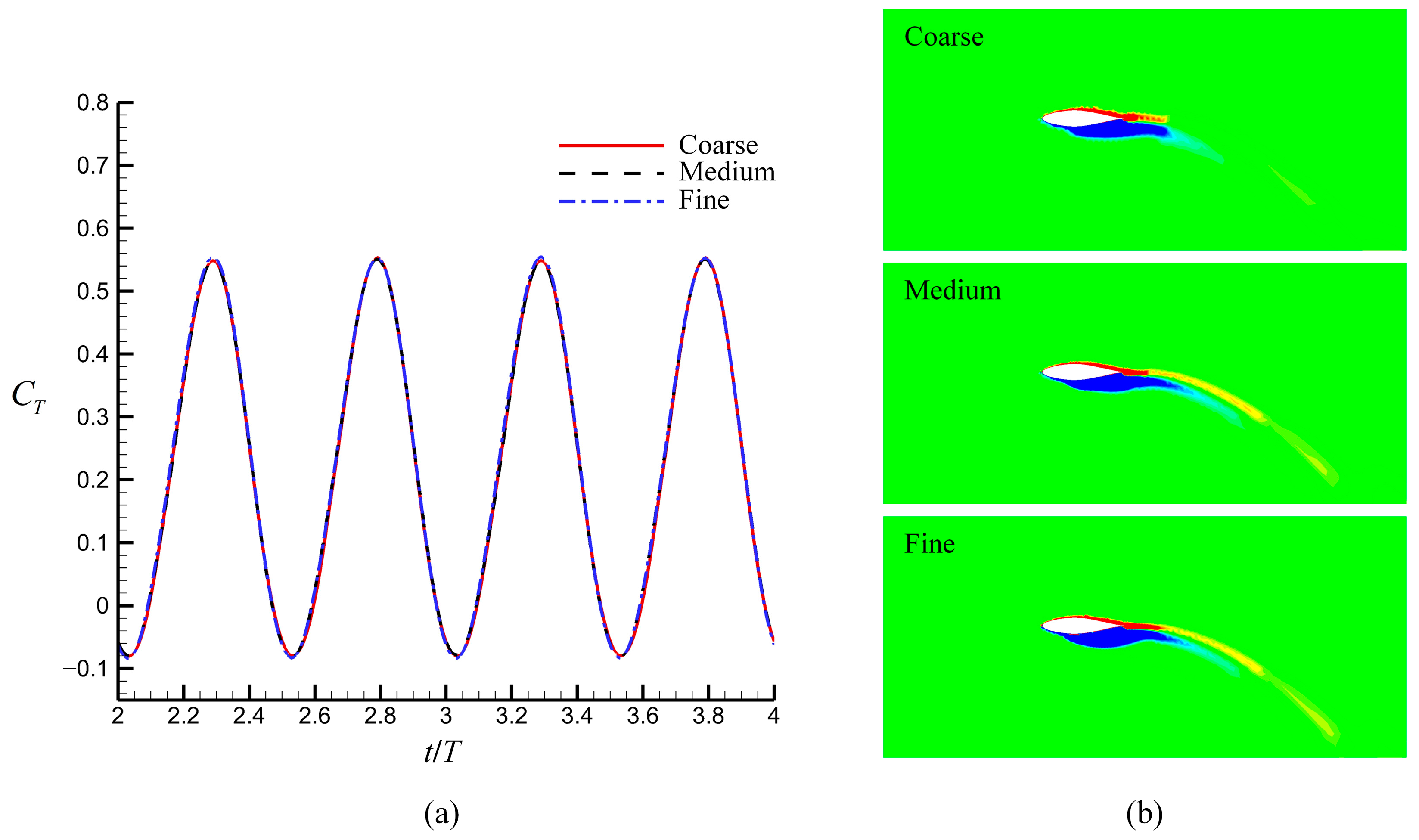
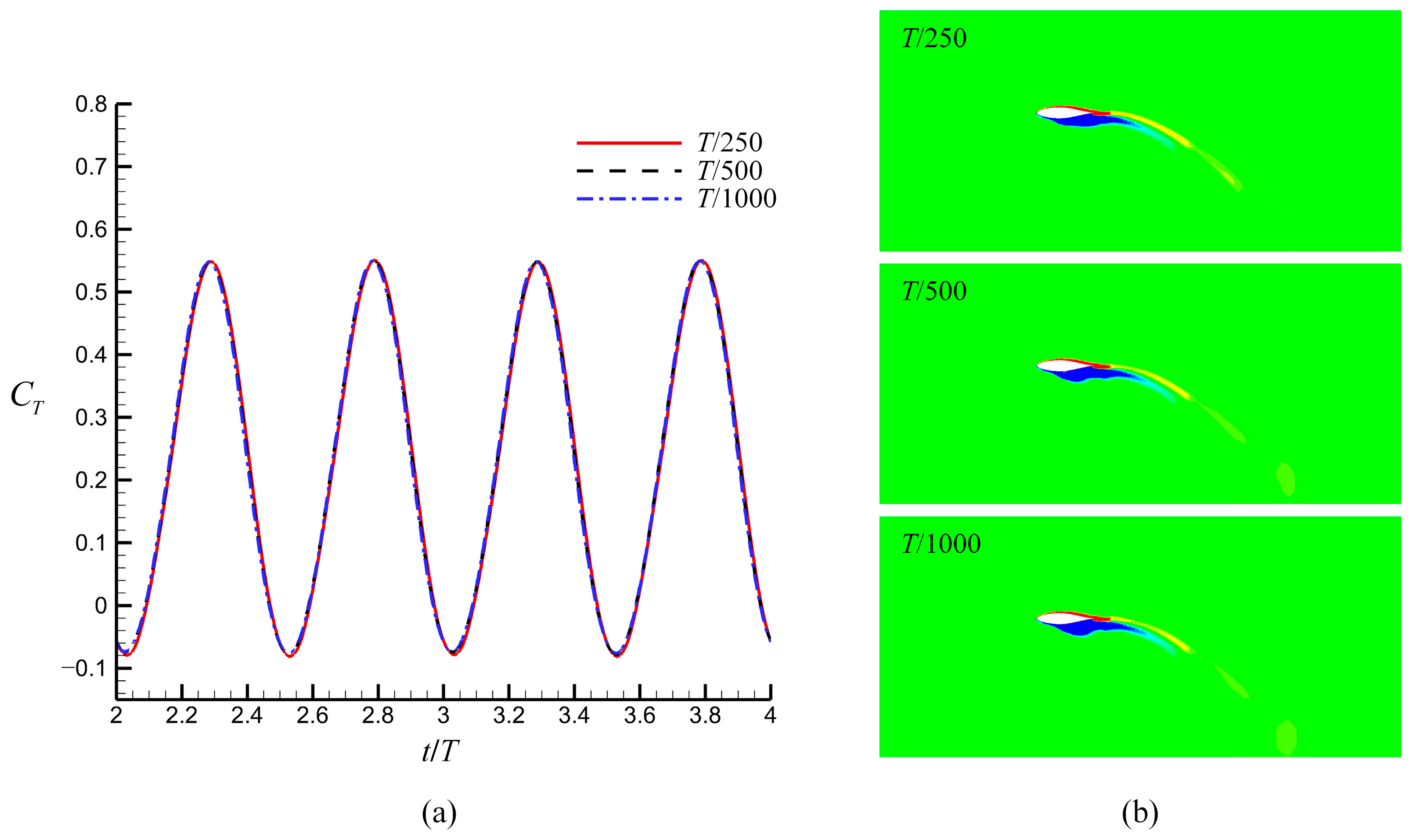
Figure 1. Shape definition of a typical foil with leading-edge tubercles. The sinusoidal leading edge consists of several sections with different local chord lengths. The peak sections have the maximum local chord length, and the trough sections have the minimum local chord length. The basic section is located between these two sections.
Jmse 11 01882 g001
Figure 2. Schematic of flapping motion. The flexible flapping motion can be decomposed into a rigid flapping motion around the x-axis and the pitch axis and a flexible deflection perpendicular to the chord direction.
Jmse 11 01882 g002
Figure 3. Vector diagram of velocity on 70% span location. The motion in the spanwise sections can be simplified to a typical 2D heave–pitch flapping motion.
Jmse 11 01882 g003
Figure 4. Profile of instantaneous angle of attack over one cycle for flexible and rigid foils. The flexibility changes the profile of the angle of attack.
Jmse 11 01882 g004
Figure 5. (a) The computational domain consists of a static cubic zone used to define the flow boundary and a moving spherical zone used to achieve the motion. (b) The domain was discretized in space using a hexahedral grid for the cubic zone and a tetrahedral mesh for the spherical zone. The sliding mesh method was used to transmit flow information through the interface.
Jmse 11 01882 g005
Figure 6. The residuals of simulations after solution convergence. The residuals of all equations are less than 0.0001 at each time step.
Jmse 11 01882 g006
Figure 7. Mesh independence validation using (a) instantaneous thrust coefficients and (b) slices of spanwise vorticity contours ( A = 0.1   c , λ = 0.25   c , S t = 0.3 , α max = 20 ° , R e = 50 , 000 ). The medium mesh was used in the present work because of the satisfactory accuracy in hydrodynamic performance and flow details.
Jmse 11 01882 g007
Figure 8. Time independence validation using (a) instantaneous thrust coefficients and (b) slices of spanwise vorticity contours. ( A = 0.1   c , λ = 0.25   c , S t = 0.3 , α max = 20 ° , R e = 50 , 000 ). Similar to the mesh independence validation, the time step size of T/500 was used in the present work because of the satisfactory accuracy in hydrodynamic performance and flow details.
Jmse 11 01882 g008
Figure 9. Comparison of instantaneous thrust measurements obtained using CFD and the experiment for a NACA0012 foil with c = 100 mm, b = 400 mm as Re = 50,000, φ 0 = 60°, St = 0.4, and α max = 40°. The CFD results match well with the experimental data [12], indicating that the numerical method can effectively predict the hydrodynamic forces of flapping foils.
Jmse 11 01882 g009
Figure 10. (a) Mean thrust coefficient, (b) power coefficient, and (c) propulsive efficiency of different tubercle shapes ( S t = 0.3 , α max = 20 ° , R e = 50 , 000 ). The tubercles led to a reduction in thrust and an increase in power consumption, which induced a reduction in propulsion efficiency. The effect was related to the shape parameters.
Jmse 11 01882 g010
Figure 11. (a) Instantaneous thrust and (b) power coefficients for different foils, and (c) the corresponding positions over one cycle ( S t = 0.3 , α max = 20 ° , R e = 50 , 000 ). The variation in peak values plays a major role in the hydrodynamic performance loss.
Jmse 11 01882 g011aJmse 11 01882 g011b
Figure 12. Slices of spanwise vorticity contour for foil (a) L025A01 and (b) baseline ( S t = 0.3 , α max = 20 ° , R e = 50 , 000 ). The separation tendency was suppressed in the peak sections and strengthened in the trough sections.
Jmse 11 01882 g012
Figure 13. Distribution of pressure coefficients (a) along the chordwise direction and (b) in the direction perpendicular to it in the peak and trough sections for the modified foil and baseline ( S t = 0.3 , α max = 20 ° , R e = 50 , 000 ). The pressure distribution of the modified foil differed significantly from that of the baseline in the peak and trough sections, which was related to the variation in performance.
Jmse 11 01882 g013
Figure 14. (a) Force diagram on sections. Pressure vector distribution on the (b) baseline, (c) peak, and (d) trough ( S t = 0.3 , α max = 20 ° , R e = 50 , 000 ). The loss of chordwise force caused by the weakening of the suction peak on the peak sections played a major role in the variation in performance.
Jmse 11 01882 g014
Figure 15. Spanwise velocity contour in the baseline section in the middle section between the peak and trough sections ( S t = 0.3 , α max = 20 ° , R e = 50 , 000 ). The tubercles allowed the flow near the leading edge to move from the lower portion to the upper portion, which was the cause of the variation in pressure distribution.
Jmse 11 01882 g015
Figure 16. (a) Mean thrust coefficients, (b) power coefficients, and (c) propulsive efficiency measured at different Strouhal numbers ( α max = 20 ° , R e = 50 , 000 ). The loss of performance decreased with the increase in St.
Jmse 11 01882 g016aJmse 11 01882 g016b
Figure 17. Distribution of pressure coefficients along the chordwise direction in peak and trough sections for modified foil and baseline at St = 0.5 (solid lines) and St = 0.3 (dashed lines) ( α max = 20 ° , R e = 50 , 000 ). The suction near the leading edge was reduced in the peak section and increased in the trough section at high Strouhal numbers, indicating that the effect of the tubercles was enhanced.
Jmse 11 01882 g017
Figure 18. (a) Mean thrust coefficients, (b) power coefficients, and (c) propulsive efficiency at different maximum angles of attack ( S t = 0.3 , R e = 50 , 000 ). Tubercles cannot benefit the flapping foils even at a high maximum angle of attack, which is different from the static foils.
Jmse 11 01882 g018
Figure 19. Distribution of pressure coefficients along chordwise direction in peak and trough sections for the modified foil and baseline at α max = 40 ° ( S t = 0.3 , R e = 50 , 000 ). The suction peaks in both the peak and the trough sections were reduced, inducing a reduction in thrust and power consumption.
Jmse 11 01882 g019
Figure 20. Slices of spanwise vorticity contours for foils (a) L025A01 and (b) baseline at α max = 40 ° ( S t = 0.3 , R e = 50 , 000 ). The presence of tubercles may expand the separation region and strengthen the flow separation in the peak and trough sections.
Jmse 11 01882 g020
Figure 21. Slices of streamwise vorticity contours for modified foil ( A = 0.1 c , λ = 0.25 c , S t = 0.3 , S t = 0.3 , R e = 50 , 000 ). Streamwise vortices similar to those of static foils were also observed on flapping foils, but similar flows did not lead to similar results.
Jmse 11 01882 g021
Table 1. Mean thrust coefficients at different mesh densities and time steps.
Mesh
No.
Mesh
Densities
Cell Numbers
(×106)
Time StepsMean Thrust
Coefficient
Relative
Error/%
e a 21 /% G C I f i n e 21 /%
3Coarse3.23T/2500.2235−0.751.060.13
2Medium6.58T/2500.2247−0.20
T/5000.22520.00
T/10000.2238−0.62
1Fine10.04T/2500.22710.86
Table 2. Simulation parameters used in the present study.
No.Foil NameA/cλ/cStαmax (°)Re
1L025A00250.0250.25[0.2, 0.5], interval 0.12050,000
0.3[15, 40], interval 550,000
2L025A0050.050.250.32050,000
3L025A00750.0750.250.32050,000
4L025A010.10.250.32050,000
5L05A00250.0250.50.32050,000
6L05A0050.050.50.32050,000
7L05A00750.0750.50.32050,000
8L05A010.10.50.32050,000
9Baseline00[0.2, 0.5], interval 0.12050,000
0.3[15, 40], interval 550,000
Table 3. Details of the parameters of motion equations expressed as Equations (2)–(4).
Stαmax (°)ω (Rad/s) Δ t (s)CFLθ0 (°)φ0 (°)B (mm)
0.2202.090.00601.0712.3327.2822.5
0.3153.140.00400.7130.0827.2822.5
0.3203.140.00400.7124.1327.2822.5
0.3253.140.00400.7118.7427.2822.5
0.3303.140.00400.7113.5727.2822.5
0.3353.140.00400.718.4727.2822.5
0.3403.140.00400.713.4027.2822.5
0.4204.190.00300.5434.8727.2822.5
0.5205.240.00240.4346.1727.2822.5
Table 4. Peak values of thrust and power coefficients.
Foil NameCTmaxRelative Error/%CPmaxRelative Error/%
L025A00250.6088−1.661.03850.80
L025A0050.5946−3.951.05352.26
L025A00750.5715−7.681.07554.39
L025A010.5505−11.081.08415.23
L05A00250.6149−0.681.04381.31
L05A0050.6085−1.711.07023.88
L05A00750.6004−3.031.09476.26
L05A010.5873−5.131.10667.41
baseline0.61910.001.03020.00
Disclaimer/Publisher’s Note: The statements, opinions and data contained in all publications are solely those of the individual author(s) and contributor(s) and not of MDPI and/or the editor(s). MDPI and/or the editor(s) disclaim responsibility for any injury to people or property resulting from any ideas, methods, instructions or products referred to in the content.

