A Method for Inverting Shallow Sea Acoustic Parameters Based on the Backward Feedback Neural Network Model

Abstract

In response to the drawbacks of low efficiency, cumbersome calculation, and easy-to-fall local optimal solutions in existing shallow water acoustic parameters inversion research, this paper proposes a shallow water acoustic parameters inversion method based on a feedback (BP) neural network model. Firstly, the theoretically predicted values of the shallow water sound pressure field are obtained through the fast field method (FFM). Secondly, a relationship model between the predicted sound pressure field and the inversion of ground sound parameter values is established based on the BP neural network model. Finally, the measured sound pressure field data are brought into the neural network model to obtain the inversion results. The application results of the method indicate that, compared to the classical simulated annealing (SA) algorithm, the BP neural network model converts the data-matching process of the optimization algorithm into the construction of a relationship model between the input data and the desired parameters, avoiding repeated matching and optimization processes. Therefore, it can directly, accurately, and efficiently output the inversion results. Under the premise of setting the same accuracy, the iteration number of the BP neural network model is reduced to 2% of the SA algorithm, cutting the calculation time to 30% of the SA algorithm. It has broad application prospects in shallow sea acoustic parameters inversion algorithms.

1. Introduction

Geoacoustic Parameters are parameters that describe the acoustic characteristics of submarine areas, including medium sound speed (including sound attenuation) and medium density. Physical parameters and sound field modeling are the bases of applications such as water sound communication and sound detection; thus, the best way to efficiently obtain shallow sea acoustic parameters has always been a hot issue in the field of geoacoustic parameters in domestic hydrology [1,2,3].

As the above-mentioned geoacoustic parameters are difficult and large-scale measurements, while the use of acoustic methods can quickly and efficiently obtain ground sound parameters in large-scale sea areas, they have received widespread attention and gained good research significance and application value [4,5,6,7,8]. In recent years, geoacoustic parameter inversion methods for use in shallow seas based on various acoustic field propagation characteristics have emerged. For example, the geoacoustic parameters inversion method is based on propagation loss [9], the geoacoustic parameters inversion method is based on acoustic signal arrival time [10], and the inversion method is based on waveguide dispersion characteristics [11].

However, the above-mentioned methods of inversion of geoacoustic parameters mainly focused on the selection of forward models for inversion problems, as well as on using various classical optimizing algorithms, such as genetic algorithms and simulated annealing algorithms. Here, the objective function is solved, and the parameters to be inverted are obtained. When applying the various classic superior algorithms, the computing of the iteration of the input data and the optimal anti-discovery interpretation will not only consume a lot of calculation time, but will also easily fall into a locally optimal solution.

In recent years, due to the superior performance of neural network algorithms in data processing, scholars have been exploring the use of neural network models as an alternative to iterative optimization methods for inversion purposes. Huang used the Convolutional Neural Network (CNN) model to measure the in the physical reaction of the earth, which successfully realized the reaction to some geological parameters [12]. Wu used a single hidden layer feedforward neural network in shallow sea water depth remote sensing inversion and obtained relatively accurate inversion results [13]. A ack propagation (BP) neural network model was applied to electromagnetic anti-disclosure by Li, and the BP nerves were used to visualize BP nerves. The network was improved to modify the algorithm of differential evolution to achieve more efficient and accurate countermeasures [14]. Wen used the BP (back propagation) neural network model to counter the effective wave high field parameters, which proves that the application neural network methods have higher counter-discovery accuracy than traditional methods [15]. Halil used typical three-layer feed forward-back propagation (FFBP) neural networks to predict daily river flows [16]. Tian utilized the tangent linear and adjoint capabilities of a neural network to develop a neural network-based four-dimensional variational data assimilation (4D-Var DA) system.

Compared to the front-oriented neural network model, the BP neural network model is a multi-layer feedforward network trained according to the error back propagation algorithm. The model is constructed according to the idea of layer-by-layer calculation and error feedback correction. In the construction, the multi-element matrix composed of weight and threshold values determines the predictive quality of the model. Even if some weight parameters fall into the local optimal, the model can be corrected by adjusting weight parameters and threshold parameters together. An established model is more stable, the number of iterations is lower, and the calculation time is faster, which can greatly facilitate the research of various inversion problems. However, little work has been completed on the application of BP neural networks to inverse research work for shallow sea acoustic parameters, and it is worthwhile strategy based on the current status of research; thus, this article proposes a method of determining counter-geoacoustic parameters based on BP neural networks, replacing the search algorithm in parameter inversion for fast and efficient inversion of the required parameters to achieve high efficiency and accurate discrimination of shallow acoustic parameters. In this study, the research object with a shallow sea sound field is taken as the research object, the relationship model between the prediction sound field and the earth sound parameters to be retrieved is established via a BP neural network, and the backward feedback neural network algorithm is used to retrieve the semi-infinite sea bottom sound parameters using sound pressure data. The main content of this paper consists of the following four parts: the first part is an overview of the sound parameters based on the acoustic pressure field; the second part introduces the BP neural network-based ground sound parameters countermeasure method; in the third part, the application effect and performance of the BP neural network model are analyzed through simulation and scaling experimental data; and the final part is the conclusion. This paper will explore inversion methods based on this logical structure.

2. Geoacoustic Parameters Inversion Method Based on the Neural Network Model

The traditional acoustic parameter inversion method based on sound pressure data in shallow sea adopted the method of matching the measured sound pressure data and the simulated value of the sound field model many times. In other words, through various optimization algorithms, a set of earth sound parameters matching the best measured sound pressures were searched using the simulation sound pressure data corresponding to several groups of earth sound parameters, with the findings being the inversion results. However, the optimization algorithm could easily fall into the local optimal solution in the application process, and every optimization process needed to be cycled into the sound field forward modeling model for iterative calculation, which greatly increased the calculation time. From the point of view of machine learning, the BP neural network model approximated the complex non-linear mapping between the acoustic pressure data set and the acoustic parameters to be inversed by repeatedly training the neural network model. In the later stage, the corresponding parameters to be inversed could be obtained only by substituting the measured acoustic pressure data into the trained model, avoiding the repeated iterative calculation through use of an optimization algorithm. This approach could not only greatly shorten the calculation time, but also had strong robustness [16].

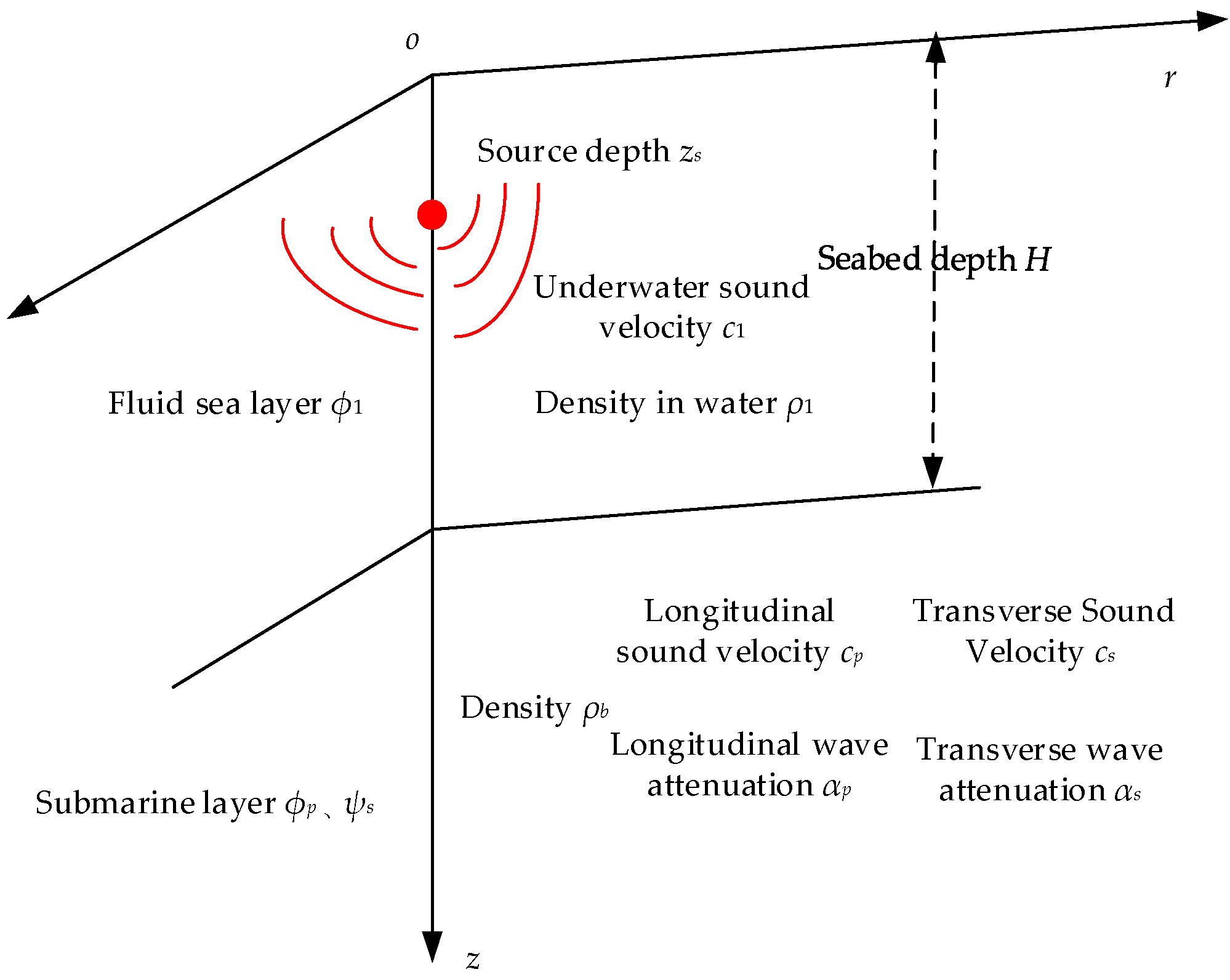
2.1. Sound Field Modeling in the Shallow Sea

Considering the shallow sea environment, the marine environment could be approximately regarded as a horizontal stratified structure composed of a seawater layer and a semi-infinite seabed layer. Therefore, a sound field model conforming to the characteristics of shallow sea environments was pre-set under the three-dimensional column co-ordinate system [17]. In this model, the harmonic point source was located on the axis of symmetry of cylindrical coordinates. Considering that the influence of seabed shear wave velocity on sound propagation in shallow sea waveguide environment could not be ignored [18,19,20], the seawater layer and seabed layer were approximately homogeneous isotropic fluid medium and elastomer medium, respectively. Due to the axial symmetry of the cylindrical co-ordinate system, the three-dimensional problem could be transformed into a two-dimensional (r, z) plane. z = 0 represented the sea surface, the downward direction of the sea surface was the positive direction of the depth Z-axis, and the positive axis of r represented the propagation direction of the sound field.

In the model, the seawater depth was set as H, and the sound source with frequency f₀ was located at z_s depth of the seawater layer. The density and sound velocity in the seawater layer were ρ₁ and c₁, respectively. The longitudinal wave sound velocity, shear wave sound velocity, density, longitudinal wave sound velocity attenuation, and shear wave sound velocity attenuation were denoted by c_p, c_s, ρ_b, α_p, and α_s, respectively. In seafloor sediment acoustics, geophysical properties can be categorized into physical properties and geoacoustic properties [21]. The geoacoustic properties primarily encompass the velocity and attenuation of P-wave and shear wave, along with sediment density. This paper focuses on inverting these five parameters as the primary targets.

Under the wave theory, each physical quantity in the above model could be represented by the displacement potential function. A model of the fluid layer displacement potential function of 1 was used. The sound pressure p = ρ₁ω²ϕ₁, (ω = 2πf₀) of this paper could be obtained by solving the displacement potential function, and the detailed theoretical derivation could be found in the literature [22]. Since the displacement potential function in the fluid layer satisfied Equation (1), its formal solution is shown in Equation (2)

$$\frac{1}{r}\frac{\vartheta }{\vartheta r}\left(r\frac{\vartheta {\varphi }_1}{\vartheta r}\right)+\frac{{\vartheta }^2{\varphi }_1}{\vartheta z^2}+k_1^2{\varphi }_1=-4\pi \delta (r,z-z_s), 0\le z\le h_1,$$

(1)

$${\varphi }_1(r,z)={\displaystyle \underset{0}{\overset{\infty }{\int }}{Z}_1(z,\xi ){\mathrm{J}}_0(\xi r)\xi \mathrm{d}\xi ,}$$

(2)

Z is the ordinary differential equation of depth z and ξ of the horizontal wavenumber, and $J_0$ is the zero-order Bessel function. According to the above-mentioned derivation results, the sound pressure field in the water layer can be expressed as follows:

$$p(r,z)={\rho }_1{\omega }^2{\displaystyle \underset{0}{\overset{\infty }{\int }}{Z}_1(z,\xi ){\mathrm{J}}_0(\xi r)\xi \mathrm{d}\xi },$$

(3)

For the solution in Equation (3), the normal mode method (NMM) and fast field method (FFM) could be used to solve Equation (3). For shallow sea environments, FFM converted the integral formula in Equation (3) into Fourier transform form for a direct solution, which was more suitable for fast calculation of sound field in the shallow sea [23]. Therefore, FFM was selected in this study to conduct a forward simulation of the sound pressure field in the above-mentioned parametric model. After the sound pressure data set p was calculated, it was substituted into the BP neural network for model training to establish a BP neural network model that could reflect the mapping relationship between the underwater sound pressure field and the ground sound parameters to be inverted in the shallow sea environment presented in Figure 1.

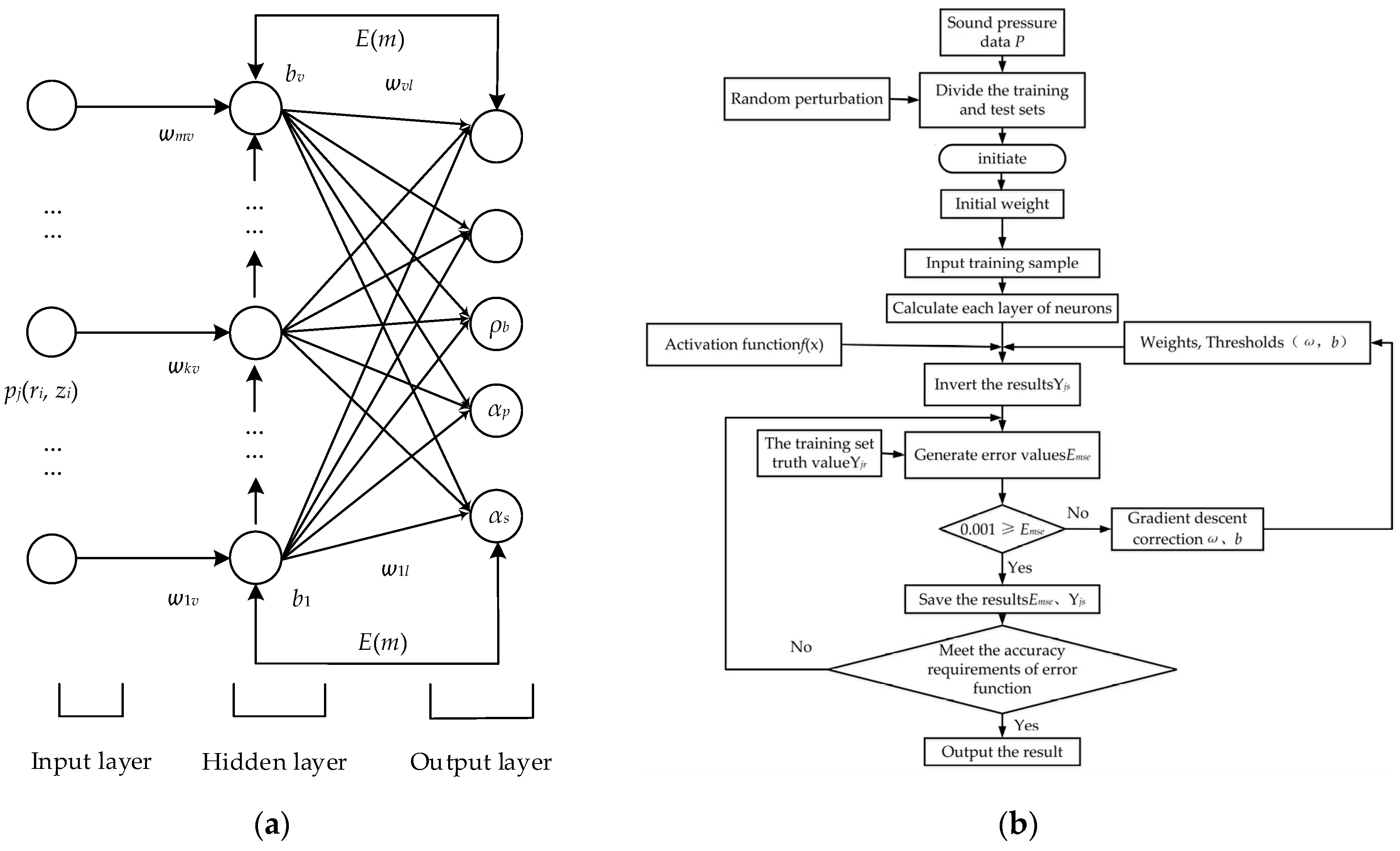
2.2. Construction of BP Neural Network

Referring to the inversion method of acoustic parameters using acoustic pressure field data, in the study of acoustic parameters inversion method in shallow sea based on BP neural network model, a group of sound pressure data p_j = [p(r₁, z₁), …, p (r_i, z_i), …, p (r_n, z_n)]_1✕n at n different receiving locations (r_i, z_i) (1 ≤ i ≤ n) was used as a group of input data in the neural network input layer. Where j = 1, 2, 3 … m, m is the total number of input sound pressure samples, namely the network input set. And, the corresponding acoustic parameters Y = [c_p, c_s, ρ_b, α_p, α_s]_m✕5 were used as label data to construct the model. Considering the complexity and computing power of the pre-set marine environment model, a single hidden layer was set in the construction of the BP neural network model. In the model, neurons in the same layer were not connected, and there were two kinds of signal communication between layers. One example was the working signal function, that is, the activation function between the input p set data and the hyperparameter matrix [w, b]. Its signal was transmitted forward from the input layer to the output layer, which could increase the non-linear factor and solve the defect of insufficient expression ability in the linear model. The other example was the error signal E_mse, which was transmitted from the output layer to the hidden layer in reverse, that is, the error function between the network model inversion results and the truth value. In this paper, the mean square error function (MSE) was designed, which was reversely transmitted layer by layer from output end to output end [24]. The activation and error functions are shown in Equations (4) and (5). For the shallow sea environment model pre-set in this paper, the structure of the BP neural network model built is shown in Figure 2a.

The forward activation function f(x) defined the output under a given input set at a neuron node and determined the content to be transmitted to the next neuron, which could be expressed as a mathematical equation to determine the output of the neural network, as shown in Equation (4). The reverse error function E_mse calculated the error between the actual inversion value Y_jinv and the expected output value Y_jsim through the error function, spread the error from the last output layer to the previous layers successively, and, finally, reduced the error by adjusting the connection weight and bias of each layer, as shown in Equation (5).

$$f\left(x\right)=\frac{1}{1+e^{-x}},$$

(4)

$$E_{mse}=\sqrt{\frac{1}{m}{\displaystyle \sum _{j=1}^m{\left[Y_{jsim}-Y_{jinv}\right]}^2}},$$

(5)

where, x is the input value of each neuron, Y_{sim, inv} = [c_p, c_s, ρ_b, α_p, α_s] is the matrix composed of parameters to be retrieved, and Y_jsim and Y_jinv represent the simulation and inversion values of group j, respectively.

After the sound pressure data p were substituted into the input layer, the hyperparameter matrix [w, b] and activation function f(x) was used to connect the neurons of each layer, and the inversion results Y_r were finally obtained through the hidden and output layers [25]. The calculation process is shown in Figure 2b, and the number of neurons in each layer could be determined according to Formula (6).

$$v=\sqrt{n+l}+\alpha ,$$

(6)

where n represents the number of nodes in the input layer, that is, the number of simulated sound pressure points; $v$ represents the number of nodes in the hidden layer; $l$ represents the number of nodes in the output layer, that is, the number of inversion earth sound parameters; and α is the constant coefficient.

The partial derivative of the weight parameter between the input set p and the hidden layer is Δwjv; the partial derivative of the weight between the hidden layer and the ground sound parameter Y is Δwvl; and η is the learning rate. In the calculation process, to judge whether the E_mse value meets the set accuracy, the iterative step t is constantly updated to the correct parameters w_jv and w_vl, as shown in Equations (7) and (8). I_kv and I_vl are, respectively, the input data of the hidden layer and the output data of the hidden layer [26]. Combined with Formula (4), the Y_inv calculation process of the obtained inversion results is shown in Formulas (9) and (10)

$$w_{kv}\left(t+1\right)=w_{kv}\left(t\right)+\Delta w_{kv},$$

(7)

$$w_{vl}\left(t+1\right)=w_{vl}\left(t\right)+\Delta w_{vl},$$

(8)

$$I_{vl}=f\left(I_{kv}\right)=f\left[{\displaystyle \sum _{i=1}^n{w}_{kv}p\left(r_i,z_i\right)}+b_v\right],$$

(9)

$$Y_{inv}=f\left(I_{vl}\right)=f\left[{\displaystyle \sum _{k=1}^v{w}_{vl}{I}_{vl}}\right],$$

(10)

In the hyperparameter matrix w = [w_jv, w_vl], v represents the number of nodes in the hidden layer; l represents the number of nodes in the output layer, that is, the number of inversion acoustic parameters; w_jv represents the weight from the input layer to the hidden layer; w_vl represents the weight from the hidden layer to the output layer; and b_v. represents the threshold of each neuron in the hidden layer, i.e., b = b_v. Since the network input error is a function of the weights and thresholds of each layer, the error function E_mse can be changed by adjusting weights. Since the principle of weight adjustment is to reduce the error continuously, the weight had to be proportional to the gradient decline of the error; thus, the method of gradient decline was adopted to update parameters. The design process is shown in Equations (11) and (12):

$$\begin{array}{l}\Delta w_{jv}=-\eta \frac{\vartheta E}{\vartheta w_{jv}}=-\eta \frac{\vartheta E}{\vartheta Y_s}\frac{\vartheta f\left(I_{vl}\right)}{\vartheta I_{vl}}\frac{\vartheta f\left[{\displaystyle \sum _{k=1}^v{w}_{vl}{I}_{jv}}\right]}{\vartheta I_{kv}}\frac{\vartheta I_{jv}}{\vartheta f\left(w_{jv}\right)}\frac{\vartheta f\left(w_{jv}\right)}{\vartheta w_{jv}}=\\ -\eta \sqrt{\frac{1}{N}{\displaystyle \sum _{m=1}^m\left[Y_{jinv}-Y_{jsim}\right]}}{f}^{\prime }\left[f\left({\displaystyle \sum _{j=1}^v{w}_{vl}{I}_v}\right)\right]w_{jv}{f}^{\prime }\left[{\displaystyle \sum _{j=1}^v{w}_{jv}p\left(r_i,z_i\right)}\right]\end{array},$$

(11)

$$\begin{array}{l}\Delta w_{vl}=-\eta \frac{\vartheta E}{\vartheta w_{vl}}=-\eta \frac{\vartheta E}{\vartheta Y_r}\frac{\vartheta f\left(I_{vl}\right)}{\vartheta I_{vl}}\frac{\vartheta f\left[{\displaystyle \sum _{j=1}^v{w}_{vl}{I}_{kv}}\right]}{\vartheta w_{vl}}=\\ -\eta \sqrt{\frac{1}{m}{\displaystyle \sum _{j=1}^m\left[Y_{jinv}-Y_{jsim}\right]}}{f}^{\prime }\left[f\left({\displaystyle \sum _{j=1}^v{w}_{vl}{I}_{kv}}\right)\right]f\left[{\displaystyle \sum _{i=1}^n{w}_{jv}p\left(r_i,z_i\right)}+b_v\right]\end{array},$$

(12)

In this paper, the seabed was simplified into two layers to establish the BP neural network inversion model. The input layer of the network structure was a group of sound pressure data p_j (r_i, z_i), i = 1, 2, 3, … n. (set the number of measured sound pressure n = 720 in simulation). The output layer was the 5 ground acoustic parameters to be inverted. According to Formula (6), by selecting different α-values during training and comparing the model performance under different α-values, α = −15 was finally determined, and the hidden layer v = 9 neurons and output layer l = 5 neurons could be determined. Here, the number of elements in the hyperparametric matrix [w, b] were 720 × 9 + 9 × 5 + 9 = 6534, which shows that 6534 weight parameters needed to be adjusted when the neural network model was constructed via the gradient descent method; thus, the neural network model approximated the complex mapping relationship between input and output to realize the inversion calculation.

The activation function, also known as the non-linear mapping function or hidden unit, is one of the most important components of a neural network. The introduction of an activation function introduced non-linear computational power into the neural network and enhanced the learning ability of the network. There were various activation functions available at this stage, which corresponded to different characteristics. There are four main types of activation functions commonly used in BPNN models: Sigmoid, Tanh, ReLU, and Softmax functions. By selecting the activation functions in the BPNN algorithm built in this paper, as the Sigmoid function was similar to the Tanh function, and the sound pressure data in the network processed at the same time had a positive sound pressure amplitude, the accuracy was set to 10⁻³ for the experiments. The Sigmoid function was used for comparison with the other two types of functions for training; as shown in Figure 3, the results show that several types of activation function were used in training. The results show that several types of activation functions have similar effects, though in comparison to other functions, the Sigmoid function had the most satisfactory training effect; thus, the activation function f(x) chosen in the paper was the Sigmoid function.

2.3. BP model Training Data Generation

Considering the variation range of ground sound parameters in the shallow sea [27], the parameter training range of the BP neural network model for ground sound parameter inversion under a pre-set environment was set as shown in

Table 1. BPNN model training set search range.

Geoacoustic Parameters	Search Range	Truth Value
c1 (m/s)	/	1500
ρ1 (g/cm3)	/	1.025
cp2 (m/s)	1800–2200	2000
cs2 (m/s)	900–1100	1000
ρb (g/cm3)	1.4–1.6	1.5
αp2 (dB·λ−1)	0.1–0.3	0.2
αs2 (dB·λ−1)	0.1–0.3	0.2

.

The simulated sound pressure field data were a set of horizontal equally spaced receiving sound pressure fields under the set sound source depth z_s = 20 m, receiving depth z_r = 10 m, and seawater depth H = 100 m. The receiving points are spaced 2 m apart, and a total of I = 720 receiving points are set.

In Table 1, $c_1$ and ${\rho }_1$ is the basic parameter of the data generated via FFT; $c_{p2}$, $c_{s2}$, ${\rho }_b$, ${\alpha }_{p1}$, and ${\alpha }_{s2}$ is the target parameter of BP neural network inversion, and the search range of inversion parameters is given in the table. The model training samples adopted are 2200 groups of sound pressure data randomly generated in each layer within the search range. In Table 1, data are obtained in batch increments, among which 2000 groups were randomly divided into training sets, and the other 200 groups were divided into test sets. Each group of the training set and its corresponding environmental sound pressure were mapped into the model one by one for training. When the error function E_mse reached the set accuracy σ = 0.01, the training was complete. In the training of the pre-set model in this paper, the change diagram of E_mse value and the number of iterations and the normalized regression diagram of training data are shown in Figure 4a and Figure 4b, respectively.

Under the above simulation conditions, after the completion of training, the value of Emse reached the setting accuracy ${10}^{-3}$ after 10 iterations, as shown in Figure 4a. In the training, most of the normalized output values fit well with the target values, and most of the output values were scattered around the fitting line, which indicated that the error reduction speed and training effect of the whole neural network were considerable, and a BP neural network model satisfying the accuracy of acoustic parameter inversion was effectively constructed. Figure 4b is a linear regression analysis of the BP neural network inversion results that, by comparing the linear regression relationship between the predicted value and the actual value, allows the performance and prediction accuracy of BP neural network to be evaluated; it can be seen that the fitting results are good. Figure 4c represents the confidence interval ribbon for neural network linear regression analysis at a 95% confidence level. Due to the narrowness of the confidence interval, data within the range of 0.50–0.54 were selected for display. This finding demonstrates that the predictions of shallow sea semi-infinite seabed acoustic parameters were highly accurate and stable at the given confidence level, indicating the strong performance of the model.

3. BP Neural Network Model Verification

After completing the training of the BP neural network model in the pre-set shallow sea environment, the actual application only needs to substitute the measured sound pressure into the BP neural network model, and all earth sound parameters to be inversed in the pre-set environment model can then be obtained.

To verify the feasibility of the BP neural network model constructed in practical application, this section will apply the simulation sound pressure data and the contraction experiment measured sound pressure data to verify the BP neural network model established above, as well as compare and analyze the performance of the BP neural network model and the classical optimization algorithm in the earth acoustic parameter inversion.

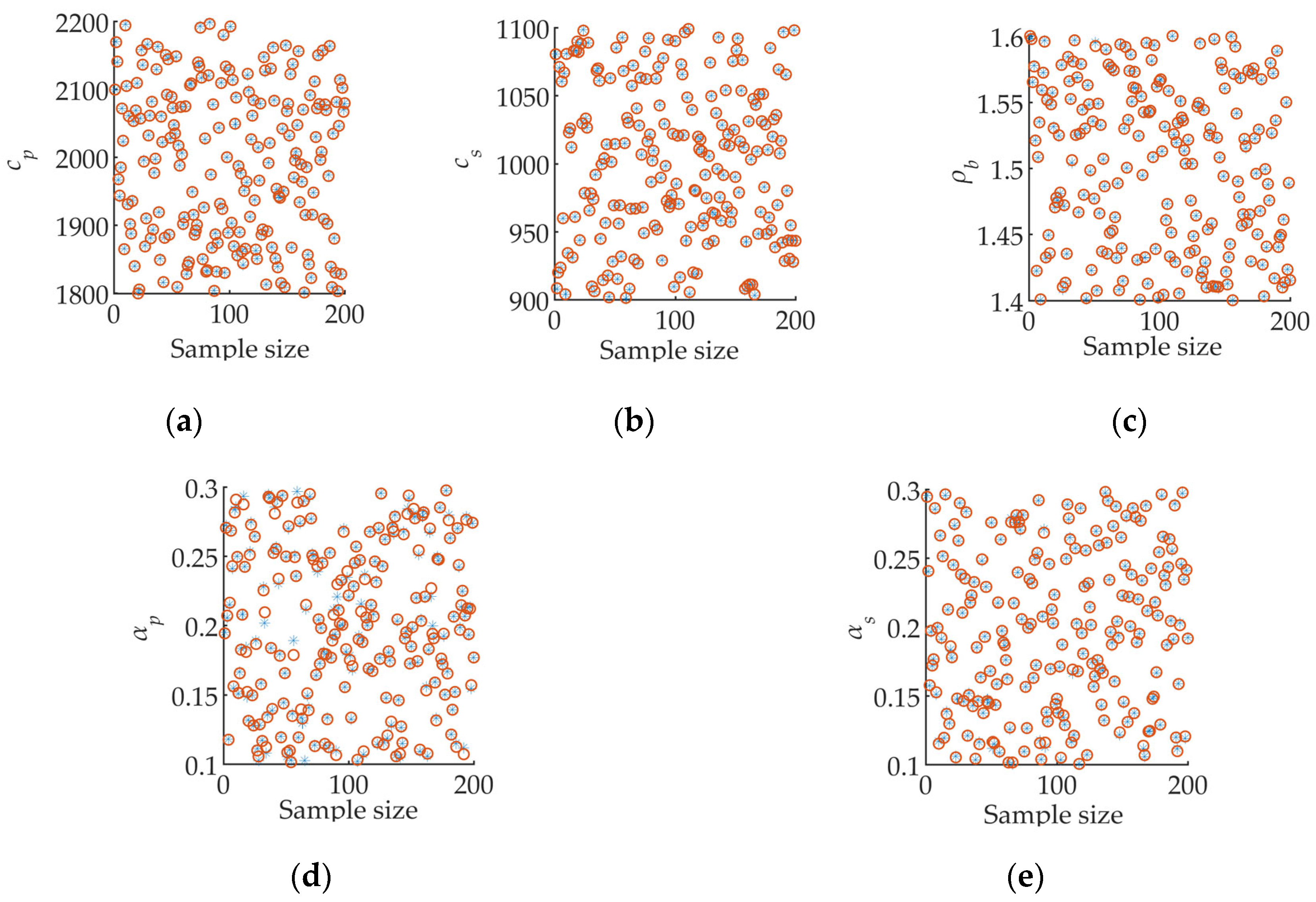
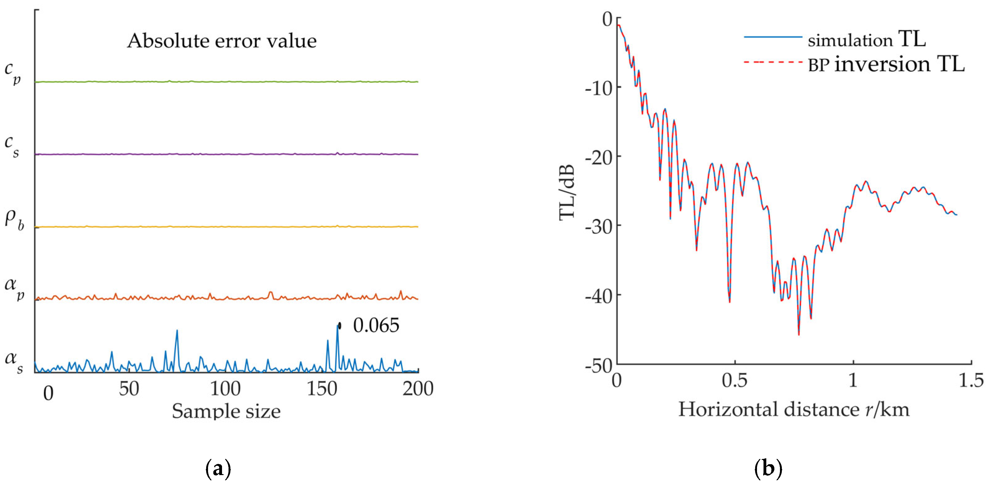
3.1. Simulation Data Verification

After completing the BP neural network model training for the inversion of five types of earth acoustic parameters under the pre-set model, the reliability of the trained neural network model is verified using the simulation data. During verification, m₁ = 200 groups of data randomly generated and divided within the parameter range of Table 1 are selected as the test set, and through the BP neural network model completed via training, the earth acoustic parameters of 200 groups of sound pressure field data were inverted. To quantify the error between the inversion results of each parameter and the pre-set truth value, the performance function R² is introduced to numerically represent the coincidence degree between the inversion value and the true value. The closer the R² value is to 1, the closer the inversion result is to the pre-set truth value.

$$R^2=\frac{{\left(m_1{\displaystyle \sum _{k=1}^{m_1}{Y}_{kinv}{Y}_{ksim}-{\displaystyle \sum _{k=1}^{m_1}{Y}_{kinv}{\displaystyle \sum _{k=1}^{m_1}{Y}_{ksim}}}}\right)}^2}{\left[m_1{\displaystyle \sum _{k=1}^{m_1}{Y}_{kinv}{}^2-{\left({\displaystyle \sum _{k=1}^{m_1}{Y}_{ksim}}\right)}^2}\right]\left[m_1{\displaystyle \sum _{k=1}^{m_1}{Y}_{ksim}{}^2-{\left({\displaystyle \sum _{k=1}^{m_1}{Y}_{kinv}}\right)}^2}\right]},$$

(13)

Figure 5 shows the comparison between the five types of results to be inversed and the pre-set truth values after 200 groups of sound pressure field data are processed. In the figure, blue “*” represents the simulation truth value, red “o” represents the inversion result, and the Y-axis represents the search range of each parameter considered to be an inversion. Due to the different sensitivities of various acoustic parameters, although the R² values of the acoustic parameter comparison results in different places are different, the agreement between the inversion results and the true values of the five earth acoustic parameters is more than 97.00%, which proves the accuracy of the simulation inversion results.

Based on Figure 5, the coincidence degree between the inversion value and the pre-set value is intuitively given. Figure 6a shows the absolute error value between the inversion value and the pre-set value of each parameter in the verification set. It can be observed from Figure 6a that the error variation trend of each parameter in the inversion model, as well as the error value of each parameter, is below 0.1 during verification. The resulting error of ρ_b, c_p, and c_s is maintained below 0.01 all of the time, and the inversion effect is excellent. The error of parameters α_p and α_s is relatively large. However, in the prediction results, the maximum error of the parameter α_p with a large error variation is only 0.065, and there is no large error fluctuation.

$$MAE=\frac{1}{n}{\displaystyle \sum _1^n\left[Y_{pre}-Y_{rea}\right]},$$

(14)

where n is the number of samples, $Y_{pre}$ is the predicted value, and $Y_{rea}$ is the simulation value, The error of MAE detection inversion results is calculated according to equation (14), and the MAE of five parameters is obtained, as shown in

Table 2. Parameter setting of the inversion algorithm.

MAE	cp	cs	ρb	αp	αs
value	2.8187	1.5010	0.0175	0.2103	0.0518

. The MAE value of the calculated model can effectively evaluate the prediction accuracy of the model, and the smaller MAE value indicates the better prediction ability of the model. It can be seen from the calculation results that the inversion error of the model is small, and the performance of the BP neural network for acoustic parameter inversion in shallow sea is good. It can be seen that the constructed BP neural network model has good and stable prediction performance for shallow sea floor acoustic parameter inversion, the calculation efficiency is efficient, and the prediction results are highly reliable.

Combined with the analysis of different sensitivities of submarine parameters shown in Figure 6a and the literature [28,29], the robustness of this BP neural network for inversion of five types of parameters is as follows: c_p, c_s, ρ_b > α_p, α_s. Figure 6b shows the comparison between the transmission loss (TL) curve calculated by setting the truth values of acoustic parameters and the TL curve calculated using inversion results. In the simulation, the calculated sound field has no influence factors, such as noise; thus, the error between the inversion result and the true value is minimal. It can be seen from the comparison that the distribution characteristics of the two curves are the same, which further proves the accuracy of the inversion results of the acoustic parameters under the pre-set model based on the BP neural network model studied in this paper.

To further discuss the application prospect of the BP neural network model in the earth acoustic parameter inversion, the BP neural network model and the classical SA algorithm are applied to the same inversion problem. To ensure the comparability of results, the loss function E_mse in BP neural network model is used as the cost function in the SA algorithm. In the calculation process, the parameter settings of the two kinds of algorithms are shown in

Table 3. Parameter settings of the inversion algorithm.

SA	BP	Parameter Setting
Population number	Training set	2000
Temperature drop rate	Learning rate η	0.01
Minimum temperature/accuracy	accuracy	0.001
Objective function	Loss function	Emse
Initial temperature	/	10

. The adaptation processes of the loss function and cost function in the two kinds of algorithms are shown in Figure 7, the dashed line represents the set accuracy, and the solid line represents the process of the accuracy decline of the two algorithms with the number of iterations.

As can be seen from the changes in the value of the objective function of the SA algorithm in the iteration shown in Figure 7a, although it quickly dropped to the accuracy of 10⁻² in the re-optimization process, it only reached the pre-set accuracy requirement of 10⁻³ after 730 iterations in total. However, the BP neural network model in Figure 7b only iterated 10 steps to reach the pre-set accuracy requirements and complete the construction of the inversion model. In terms of model iteration times, the computational efficiency of the neural network is much higher than that of inversion determined using only an optimization algorithm. After repeating the calculation many times, it is found that the two algorithms can perform a single inversion of the earth’s acoustic parameters in the simulation conditions, and the comparison of the time and the number of model iterations is given in

Table 4. Comparison of the inversion algorithm’s results.

Inversion Algorithm	cp	cs	ρb	αp	αs	CPU Usage Time	Number of Iterations	Calculation Accuracy
Truth value	2000.00	1000.00	1.50	0.20	0.20	/	/	/
SA algorithm	2000.0922	999.5928	1.4993	0.2005	0.2110	10 ± 5 min	780 ± 50	10–3
Relative error of SA	0.0046%	0.041%	0.047%	0.25%	5.5%	/	/	/
BP neural network model	1999.1283	999.6819	1.5003	0.1998	0.2015	3 ± 1.5 min	10 ± 5	10–3
Relative error of BP model	0.043%	0.032%	0.020%	0.10%	0.75%	/	/	/

.

It can be seen from the simulation comparison that the error between the inversion results obtained via the SA algorithm and BP neural network model and the true value is less than or equal to 10⁻³. The inversion values obtained via the two methods are compared to the true values, the accuracy of the inversion results of the BP network model is higher than those of the SA algorithm, c_s, ρ_b, α_p, and α_s, and the BP neural network is more stable in relative error control, having less fluctuation.

In this paper, the BP neural network model and the classical SA algorithm are used for the ground acoustic multi-parameter inversion. From the error analysis, the SA algorithm has different resolutions of multiple parameters in multi-parameter solving problems; thus, it is inconsistent in solving accuracy, and the calculation time is too long. However, the BP neural network model only uses 2000 groups of data for training, and the number of iteration steps in the operation is 1.3% of the SA algorithm, thus achieving considerable accuracy requirements. Although there are also similar differences in the robustness of different parameter inversions, all inversion parameters can reach the same accuracy.

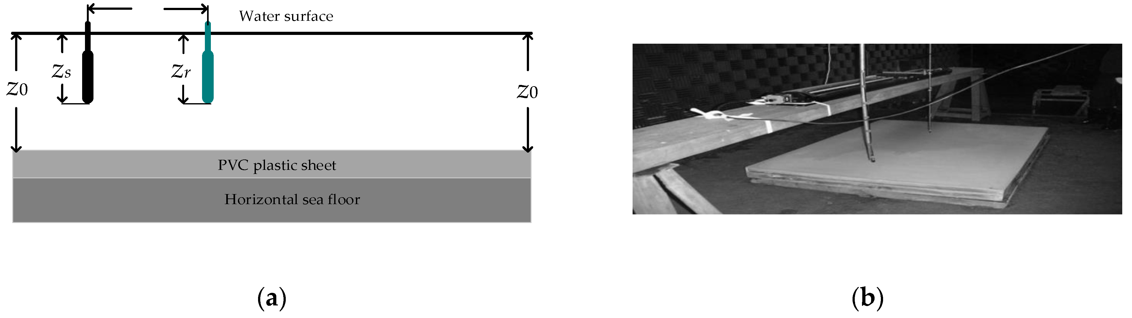
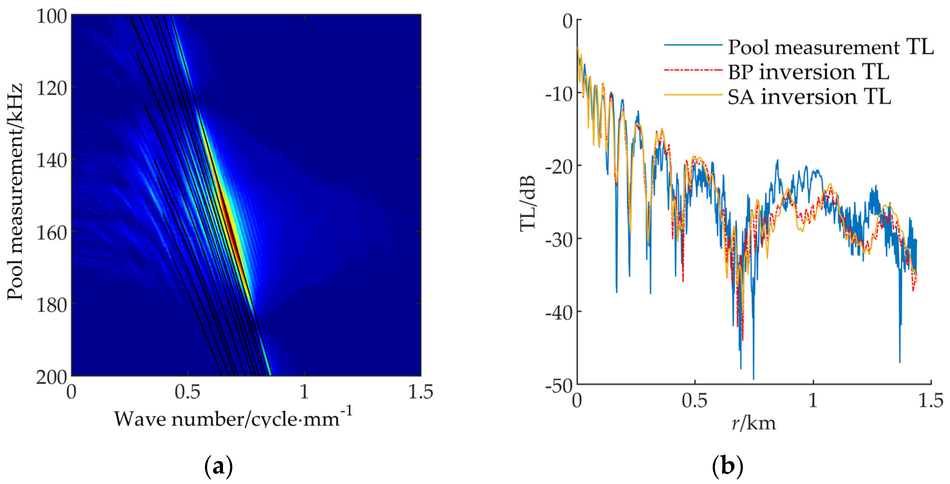
3.2. Validation of Measured Data

Based on simulation verification of the accuracy and applicability of the proposed method, the feasibility of the proposed inversion method in practical application is further verified in this section, in combination with the experimental data of the muffler pool shrinkage. The experiment was carried out in an anechoic pool using a uniform and high-hardness PVC board (polyvinyl chloride polymer, measured density of 1.20 g/cm⁻³) “semi-infinite elastic seabed” [30,31,32,33]. In the experiment, the sound source depth is z_s = 87 mm, the receiving depth is z_re = 84 mm, and the water depth is H = 182 mm. The sound velocity in water c₁ is calculated based on the sound velocity empirical formula, considering the water temperature under standard atmospheric pressure 11.5 ℃, and c₁ = 1450.212 m/s is obtained. During the process, the sound source was fixed, and pulse signals of f = 155 kHz were transmitted. The receiving hydrophone was placed on the movable walking frame and received by a single TC4038 standard hydrophone at different positions at equal intervals. The sampling frequency of the acquisition card is f_s = 20 MHz. The hydrophone moves away from the sound source by 2 mm each time to record data. A total of 720 position points were measured during the experiment, and the average value of each position was measured 10 times as the final test data. Figure 8 shows the experimental schematic diagram of the scale reduction experiment and the layout of the experimental equipment, and the propagation loss in the environment of the experimental tank is measured in Figure 8.

The BP neural network model established in this paper and the classical SA algorithm were used to invert the measured data of the water tank.

Table 5. Inversion results of the measured data.

Geoacoustic Parameters	Search Range	Inversion Results of BP	Inversion Results of SA
cp (m/s)	2200–2500	2386.6	2379.6
cs (m/s)	1100–1300	1136.2	1191.1
ρb (g/cm3)	1.0–1.8	1.21	1.23
αp (dB·λ−1)	0.1–1.1	0.43	0.58
αs (dB·λ−1)	0.1–1.1	1.01	0.77

shows the search range of five earth-sound parameters and the results of inversion using the BP neural network and SA methods, respectively. In Figure 9a,b, combined with the inversion results, the comparison diagram of the measured TL curve and dispersion curve in the experiment is given.

Figure 9a shows the frequency–wave number spectrum measured by the water tank. It can be seen from the spectrum that the energy of the received sound pressure signal is mainly distributed in the range of 145−175 kHz, and its peak value is around 155 kHz, which is consistent with the performance index of the sound source set in the experiment. Figure 9b shows the propagation loss comparison curves of the BP neural network model and SA inversion algorithm on the measured data. It can be seen from the comparison curve in the figure that the TL curves of the two methods are consistent with the measured TL curves. Combined with the inversion results given in Table 5, it can be seen that the inversion results of c_p, c_s, ρ_b, α_p, and α_s of the BP neural network model and SA algorithm are very close to each other, which further verifies the applicability of the BP neural network model in actual earth acoustic parameter inversion research. When the density ρ_b = 1.20 g/cm⁻³ of the plastic plate selected in the pool experiment is known, the inversion values of the BP neural network model and SA inversion algorithm are 1.21 g/cm⁻³ and 1.23 g/cm⁻³, respectively, and the relative error values are 0.83 and 2.5%, respectively. Combined with Figure 9b, the BP neural network model can achieve the set target accuracy compared to the SA inversion algorithm, though the efficiency is only 30% of that of the SA inversion algorithm. It can be concluded that the BP neural network algorithm will have a broader application prospect and development space in the inversion of acoustic parameters.

4. Conclusions

• This study proposes an inversion method for five ground acoustic parameters using the back propagation (BP) neural network model. The method utilizes the fast field method (FFM) to predict the shallow sea sound pressure field and establishes a relationship model between the predicted sound pressure field and the ground sound parameters. By inputting measured sound pressure field data into the neural network model, accurate inversion results for the five subsea acoustic parameters are obtained. The method is validated through simulation and experimental data.
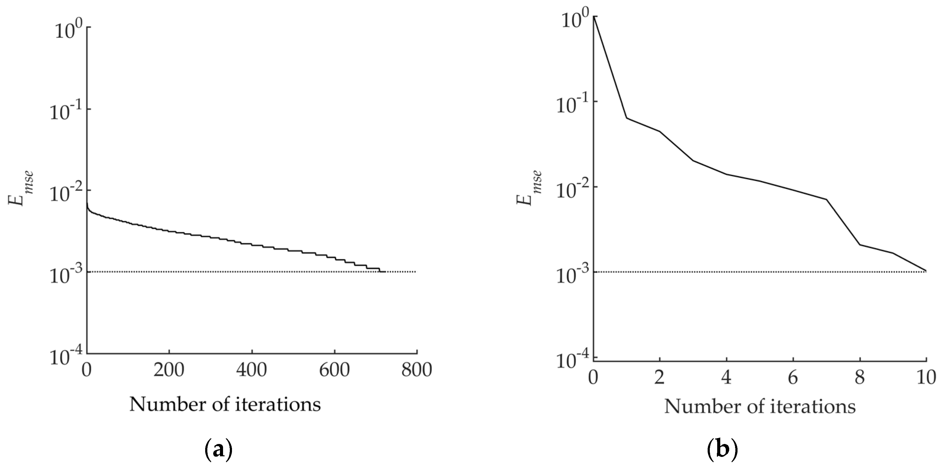
• Compared to existing optimization algorithms, the neural network-based inversion method for acoustic parameters in the shallow sea offers higher efficiency and avoids local optima. By adjusting the weights and thresholds of neurons, the neural network quickly approximates the mapping relationship between measured data and the parameters to be inverted. Among them, all kinds of weights in the hyperparameter matrix [w, b] determine the establishment process of the network, effectively avoiding the resulting error caused by the local optimal of a single parameter. The established network effectively mitigates errors caused by local optima in individual parameters. With comparable accuracy requirements, this method improves inversion efficiency, enables direct application to similar problems, eliminates redundant calculations, and enhances the overall efficiency and applicability.
• For the acoustic pressure field in water, the five acoustic parameters, i.e., shallow sea bottom density, p-wave velocity, S-wave velocity, p-wave velocity attenuation, and S-wave velocity attenuation, have different effects. It can be seen from the results of this paper that the accuracy of the inversion results of the two algorithms for S-wave acoustic velocity c_p, i.e., p-wave acoustic velocity c_s and the density ρ_b of the sedimentary layer, are all higher than S-wave attenuation α_p and p-wave attenuation α_s, which accords with the physical property that the first three types of acoustic parameters have a greater influence on the shallow sea sound pressure field in forward modeling. Due to the complexity of the shallow sea bottom and the influence of various noises on the distribution of sound fields in seawater, the actual calculation results may be somewhat different to the real situation. In addition, the coupling relationship between the physical parameters of the seabed and the sensitivity relationship of each parameter are also factors that affect the accuracy of the calculation. Given the above deficiencies, the BP neural network model is further optimized by adjusting the neural network structure and adding random noise to the subsequent research to obtain the earth acoustic parameter inversion model with stronger reliability. At the same time, the influence of network setting parameters on the accuracy of inversion results is further studied and discussed in detail. This paper focuses on conducting sound field simulation calculations and submarine sediment parameter inversion using a shallow sea semi-infinite seabed model. In future research, we plan to incorporate multi-layer seabed models to improve the parameter inversion process based on real-world seabed conditions. Additionally, we will explore the integration of GA and other optimization algorithms to enhance the performance of the BP neural network algorithm and improve the accuracy of predictions. These advancements aim to enhance the authenticity and effectiveness of the inversion process.

References

1. Ren, Q.Y.; Piao, S.C.; Ma, L. Geoacoustic inversion using ship noise vector field. J. Harbin Eng. Univ. 2018, 39, 236–240. [Google Scholar]
2. Li, Z.L.; Zhang, R.H. Hybrid geoacoustic inversion method and its application to different sediments. J. Acoust. Soc. Am. 2017, 142, 2558. [Google Scholar] [CrossRef]
3. Ma, L.; Wen, M.H.; Qiao, G. Design and Application of Acoustic Communication System for Unmanned Undersea Vehicle. J. Unmanned Undersea Syst. 2018, 26, 449–455. [Google Scholar]
4. Gerstoft, P. Inversion of seismoacoustic data using genetic algorithms and aposteriori probability distributions. J. Acoust. Soc. Am. 1994, 95, 770–782. [Google Scholar] [CrossRef] [Green Version]
5. Dragna, D.; Blanc-Benon, P. Sound propagation over the ground with a random spatially-varying surface admittance. J. Acoust. Soc. Am. 2017, 142, 2058–2072. [Google Scholar] [CrossRef] [PubMed] [Green Version]
6. Dall’Osto, D.R.; Dahl, P.H. Geoacoustic inversion based on particle velocity. J. Acoust. Soc. Am. 2016, 139, 2125. [Google Scholar] [CrossRef]
7. Li, Q.Q.; Yang, F.L.; Zhang, K. Moving source parameter estimation in an uncertain environment. Acta Phys. Sin. 2016, 65, 155–163. [Google Scholar]
8. Becker, K.M. Geoacoustic Inversion in Laterally Varying Shallow Water Environments Using High-Resolution Wavenumber Estimation. Ph.D. Thesis, Massachusetts Institute of Technology, Cambridge, MA, USA, 2017. [Google Scholar]
9. Qiu, C.J.; Chen, Y.; Ma, S.Q.; Zhou, M. Research on vertical correlation of deep sea sound field based on reliable acoustic path. Acoust. Technol. 2019, 3, 270–277. [Google Scholar]
10. Wang, Z.J. Inversion for Sea Bottom Parameters Using Vertical Array. Bachelor’s Thesis, Harbin Engineering University, Harbin, China, 2008. [Google Scholar]
11. Song, W.H.; Wang, P.Y. High-Resolution Modal Wavenumber Estimation in Range-Dependent Shallow Water Waveguides Using Vertical Line Arrays. J. Acoust. Soc. Am. 2022, 152, 691–705. [Google Scholar] [CrossRef]
12. Huang, X.R.; Dai, Y.; Xu, Y.G. Seismic Inversion Experiments Based on Deep Learning Algorithm Using Different Datasets. J. Southwest. Pet. Univ. 2020, 42, 16–25. [Google Scholar]
13. Wu, Z.Q.; Mao, Z.H.; Wang, Z. Research on China’s Coastal GPS Stations for Tide Coefficients. Hydrogr. Surv. Charting 2019, 39, 11–15. [Google Scholar]
14. Li, R.Y.; Zhang, H.Q.; Zhuang, Q. BP Neural Network and Improved Differential Evolution for Transient Electromagnetic Inversion. Comput. Geosci. 2020, 137, 104–106. [Google Scholar] [CrossRef]
15. Wen, B.Y.; Tang, W.C.; Tian, Y.W. Significant Wave Height Field Inversion of High Frequency Radar Based on BP Neural Network. J. Huazhong Univ. Sci. Technol. 2021, 49, 114–119. [Google Scholar]
16. Zhu, H.H.; Xiao, R.; Zhu, J. Influence of Internal Solitary Waves on Sound Propagation in Three-dimensional Shallow Sea. Acta Acust. 2021, 46, 365–374. [Google Scholar]
17. Tian, X.; Conibear, L.; Steward, J. A Neural-Network Based MPAS—Shallow Water Model and Its 4D-Var Data Assimilation System. Atmosphere 2023, 14, 157. [Google Scholar] [CrossRef]
18. Burgan, H.I. Comparison of different ANN (FFBP, GRNN, RBF) algorithms and Multiple Linear Regression for daily streamflow prediction in Kocasu River, Turkey. Fresenius Environ. Bull. 2022, 31, 4699–4708. [Google Scholar]
19. Hamilton, E.L. Geoacoustic modeling of the sea floor. J. Acoust. Soc. Am. 1980, 68, 1313–1340. [Google Scholar] [CrossRef]
20. Frederick, C.; Villar, S.; Michalopoulou, Z.H. Seabed classification using physics-based modeling and machine learning. J. Acoust. Soc. Am. 2020, 148, 859–872. [Google Scholar] [CrossRef]
21. Komen, D.; Neilsen, T.B.; Howarth, K. Seabed and range estimation of impulsive time series using a convolutional neural network. J. Acoust. Soc. Am. 2020, 147, 403–408. [Google Scholar] [CrossRef]
22. Li, Q.Q.; Khan, S.; Yang, F.L.; Xu, Y.; Zhang, K. Compressive Acoustic Sound Speed Profile Estimation in the Arabian Sea. Mar. Geod. 2020, 43, 603–620. [Google Scholar] [CrossRef]
23. Li, L.J.; Sun, H.X.; Liu, Y.R. Numerical analysis on radiation acoustic field of ideal sound source. Mach. Des. Manuf. 2019, 4, 192–195. [Google Scholar]
24. Zhu, H.H.; Zheng, G.X.; Zhang, H.G. Study on propagation characteristics of low frequency acoustic signal in shallow water environment. J. Shanghai Jiao Tong Univ. 2017, 51, 1464–1472. [Google Scholar]
25. Stoll, R.D.; Kan, T.K.G. Reflection of acoustic waves at a water-sediment interface. J. Acoust. Soc. Am. 1998, 70, 149–156. [Google Scholar] [CrossRef]
26. Li, M.Z.; Li, Z.L.; Li, Q.Q. Geoacoustic inversion for bottom parameters in a thermocline environment in the northern area of the South China Sea. Acta Acust. 2019, 44, 321–328. [Google Scholar]
27. Zhou, J.B.; Tang, J.; Yang, Y.X. A study on the estimation of source bearing in an ASA wedge: Diminishing the estimation error caused by horizontal refraction. J. Mar. Sci. Eng. 2021, 9, 1449. [Google Scholar] [CrossRef]
28. Zhang, X.; Yang, P.; Zhou, M. Multireceiver SAS imagery with generalized PCA. IEEE Geosci. Remote Sens. Lett. 2023, 99, 1. [Google Scholar] [CrossRef]
29. Zhou, J.B. Analysis of ambient noise spectrum level correlation characteristics in the China Sea. IEEE Access 2020, 8, 7217–7226. [Google Scholar] [CrossRef]
30. Li, X.M.; Piao, S.C.; Zhang, M.H. A passive source location method in a shallow water waveguide with a single sensor based on Bayesian theory. Sensors 2019, 19, 1452. [Google Scholar] [CrossRef] [Green Version]
31. Zhang, X.; Wu, H.; Sun, H.; Ying, W. Multireceiver SAS imagery based on monostatic conversion. IEEE J.-STARS 2021, 14, 10835–10853. [Google Scholar] [CrossRef]
32. Zheng, G.X.; Piao, S.C.; Zhu, H.H. Bayesian inversion method of geo-acoustic parameter in shallow sea using acoustic pressure field. J. Harbin Eng. Univ. 2021, 42, 497–504. [Google Scholar]
33. Feng, X.; Zhou, M.Z.; Zhang, X.B. Variational Bayesian Inference Based Direction of Arrival Estimation in Presence of Shal-low Water Non-Gaussian Noise. J. Electron. Inf. Technol. 2022, 44, 1887–1896. [Google Scholar]
Figure 1. Schematic diagram of the sound field model in cylindrical co-ordinates.
Jmse 11 01340 g001
Figure 2. Inversion via the BP neural network: (a) BP neural network model for model inversion; (b) flow chart of BP neural network acoustic parameter inversion.
Jmse 11 01340 g002
Figure 3. Comparison of training effect of activation function.
Jmse 11 01340 g003
Figure 4. Training process diagram: (a) training error variation chart; (b) regression analysis; (c) partial 95% confidence interval ribbon plot.
Jmse 11 01340 g004
Figure 5. Comparison between inversion results and pre-set values of 200 test sets: (a) cp; (b) cs; (c) ρb; (d) αp; (e) αs.
Jmse 11 01340 g005
Figure 6. Parameter error and TL comparison: (a) error fluctuation of each parameter in the test; (b) TL curve comparison under simulation conditions.
Jmse 11 01340 g006
Figure 7. Variation in the fitness curves with the number of iterations under the two algorithms: (a) fitness curve in the process of solving the SA algorithm; (b) fitness curve in the process of solving the BP neural network model.
Jmse 11 01340 g007
Figure 8. Schematic diagram of the experimental process: (a) experimental diagram; (b) layout of the experimental equipment.
Jmse 11 01340 g008
Figure 9. Inversion effect comparison: (a) comparison between the BP inversion and measured dispersion curve; (b) BP and SA inversion TL curve compared to the measured TL.
Jmse 11 01340 g009