A Subaperture Motion Compensation Algorithm for Wide-Beam, Multiple-Receiver SAS Systems

Abstract

Uncompensated motion errors can seriously affect the imaging quality of synthetic aperture sonars (SASs). In the existing line-by-line motion compensation (MOCO) algorithms for wide-beam multiple-receiver SAS systems, the approximate form of the range history error usually introduces a significant approximation error, and the residual two-dimensional (2D) range cell migration (RCM) caused by aperture-dependent motion errors is not corrected, resulting in the severe defocus of the image. In this paper, in the presence of translational and rotational errors in a multiple-receiver SAS system, the exact range history error concerning the five-degree-of-freedom (DOF) motion errors of the sway, heave, yaw, pitch, and roll under the non-stop-hop-stop case is derived. Based on this, a two-stage subaperture MOCO algorithm for wide-beam multiple-receiver SAS systems is proposed. We decompose the range history error into the beam-center term (BCT) and the residual spatial-variant term (RSVT) to compensate successively. In the first stage, the time delay and phase error caused by the BCT are compensated receiver-by-receiver through interpolation and phase multiplication in the azimuth-time domain. In the second stage, the data of a single pulse are regarded as a subaperture, and the RSVT is compensated in the subaperture range-Doppler (RD) domain. We divide the range into several blocks to correct RCM caused by the RSVT in the subaperture RD domain, and the phase error caused by the RSVT is compensated by phase multiplication. After compensation, the wide-beam RD algorithm is used for imaging. Simulated and real-data experiments verify the superiority and robustness of the proposed algorithm.

1. Introduction

The synthetic aperture sonar [1,2,3,4,5,6] (SAS) deviates from its nominal trajectory, and the turbulence of the propagation medium will disturb the phase of the detected echoes, resulting in poor imaging quality, so motion compensation (MOCO) is necessary. There are two main groups of MOCO methods: One is the echo-based MOCO method [7,8,9,10,11], which is called the displaced phase center antenna (DPCA) algorithm. The DPCA algorithm is computationally expensive, and the estimation error accumulates with the number of pulses [12]. The other MOCO method is based on motion sensors [13,14,15,16,17,18,19,20,21]. Although the motion-sensor-based compensation method is coarse, it is still an effective and robust MOCO method [14]. This paper mainly discusses the motion-sensor-based compensation method.

The motion errors of the multiple-receiver SAS can be classified into two groups: (1) translational with three degrees of freedom (surge, sway, and heave) and (2) rotational with another three degrees of freedom (yaw, pitch, and roll) [22]. The surge is introduced by non-zero along-track acceleration, which can be compensated by the real-time adjustment of pulse repetition frequency (PRF). We assume that the surge has been compensated in this paper. The sway will cause range history error for all receivers, which is regarded as an important type of motion error. The influences of the heave and pitch cannot be ignored at a short range and large elevation angle. The yaw and pitch will cause large range history errors for edge receivers in the case of long arrays. In addition, the range history error caused by the roll also needs to be discussed. Therefore, this paper analyzes and compensates the range history error caused by the five-degree-of-freedom (DOF) motion errors of the sway, heave, yaw, pitch, and roll.

In the case of narrow-beam systems, typical two-step MOCO [23] or one-step MOCO [24] can achieve high-resolution imaging for azimuth-invariant and range-variant MOCO. Generally, the above compensations are allowed for systems with a beam width of less than 10° [25]. However, with higher azimuth resolution [26] and lower frequency [27,28,29], the beam of SASs becomes wider (such as HISAS 1030, HISAS 2040, etc.). The wide beam invalidates the beam-center approximation of the two-step MOCO and one-step MOCO methods, resulting in residual azimuth-variant motion errors after the beam-center MOCO. The above problem also exists in wide-beam synthetic aperture radar (SAR) systems. There are several methods for compensating for the residual azimuth-variant phase errors, including subaperture compensation [30], subaperture topography- and aperture-dependent (SATA) [31], frequency division (FD) [32,33], and precise topography- and aperture-dependent (PTA) [34,35] algorithms. In the research of MOCO for wide-beam, multiple-receiver SAS systems, Callow et al. [18] proposed a subaperture compensation algorithm. Callow takes the data of a single pulse as a subaperture and compensates the motion errors in the wavenumber domain of the subaperture. However, there are two main challenges using the above algorithms for the wide-beam, multiple-receiver SAS MOCO.

(1) In the case of multiple-receiver configuration and non-stop-hop-stop, the exact range history is a complex function concerning the five-degree-of-freedom (DOF) motion errors of the sway, heave, yaw, pitch, and roll. However, the existing range history suitable for wide-beam SAR MOCO is the approximate form in the case of single-receiver configuration (only translational motion errors exist) and stop-hop-stop. Although the range history derived from [18] is based on multiple-receiver configuration, the heave and pitch are ignored. The multiple-receiver SAS MOCO using the approximate range history error will degrade the image focus severely. Therefore, the exact range history error is crucial for multiple-receiver SAS MOCO.

(2) In typical wide-beam SAR systems, the residual range history error after beam-center MOCO is azimuth-variant and range-invariant; this causes azimuth-variant phase errors but does not result in range cell migration (RCM). However, in the wide-beam SAS systems, because of the centimeter-level range resolution and a larger covering range of the elevation, the residual range history error after beam-center MOCO causes not only the range-variant and azimuth-variant phase error but also the range-variant and azimuth-variant RCM. This residual two-dimensional spatial-variant RCM should also be compensated for in wide-beam SAS systems, which differs from the phase error that is compensated only in wide-beam SAR systems.

In this paper, we derive the exact range history error concerning the five-DOF motion errors in the non-stop-hop-stop case and develop a two-stage subaperture MOCO algorithm to compensate for the beam-center term (BCT) and the residual spatial-variant term (RSVT) successively. The BCT changes rapidly with receivers and is compensated receiver-by-receiver in the first stage. The RCM and phase errors caused by the BCT are compensated through interpolation and phase multiplication, respectively. The RSVT is 2D spatial-variant but changes slowly with the receivers. Therefore, the difference between receivers can be ignored, and the RSVT of the reference receiver can be uniformly used to compensate in the subaperture RD domain. In the second stage, the data of a single pulse are regarded as a subaperture, and a short Fourier transform (FT) is performed to enter the RD domain to compensate for the RSVT. The RSVT is approximately proportional to the cosine of the azimuth angle off the beam center, and the azimuth angle can be obtained through the Doppler frequency. The time delay error caused by the RSVT usually spans several range cells, causing additional 2D spatial-variant RCM. We correct the residual 2D spatial-variant RCM by dividing the range into blocks and compensate for the phase error caused by the RSVT through phase multiplication. Finally, the subapertures are stitched along the azimuth after the azimuth inverse Fourier transform (IFT). After compensation, the pre-processing scheme in [36] is adopted to convert the data of the wide-beam, multiple-receiver SAS into the monostatic SAS equivalents, and then the RD algorithm [37] is used for imaging.

The main innovations of the proposed algorithm are as follows:

(1) In the case of multiple-receiver configuration and non-stop-hop-stop, the exact range history for motion errors is derived, which include five kinds of errors: sway, heave, yaw, pitch, and roll. The compensation performance using the exact expression is much better than using the existing range histories.

(2) Because of the centimeter-level range resolution and a larger covering range of elevation in the wide-beam SAS, the residual RCM after beam-center MOCO is 2D spatial-variant. In the proposed subaperture MOCO algorithm, this residual 2D spatial-variant RCM is compensated by dividing the range into blocks.

The remainder of this paper is organized as follows. In Section 2, the exact expression of range history error is derived. In Section 3, the spatial-variant characteristics of the range history error are analyzed, providing a basis for the subsequent compensation scheme. In Section 4, the detailed process of the algorithm is shown, as well as the applicable conditions and computational efficiency. Section 5 compares the compensation performance of this algorithm with the wide-beam compensation algorithm in [18] and the classic SATA algorithm through simulated data and real data, to verify the effectiveness and robustness of this algorithm. Section 6 serves as a summary of this paper.

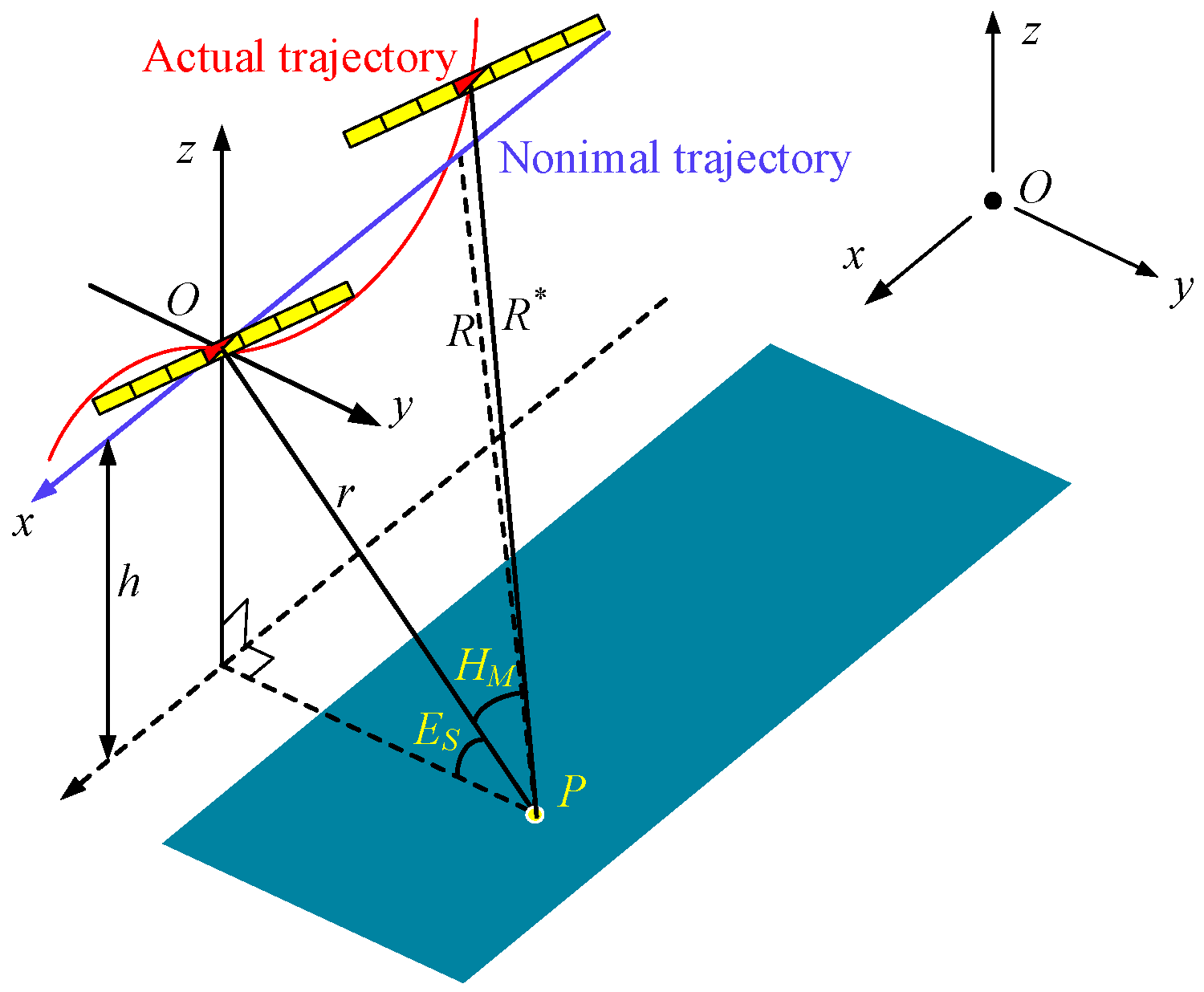
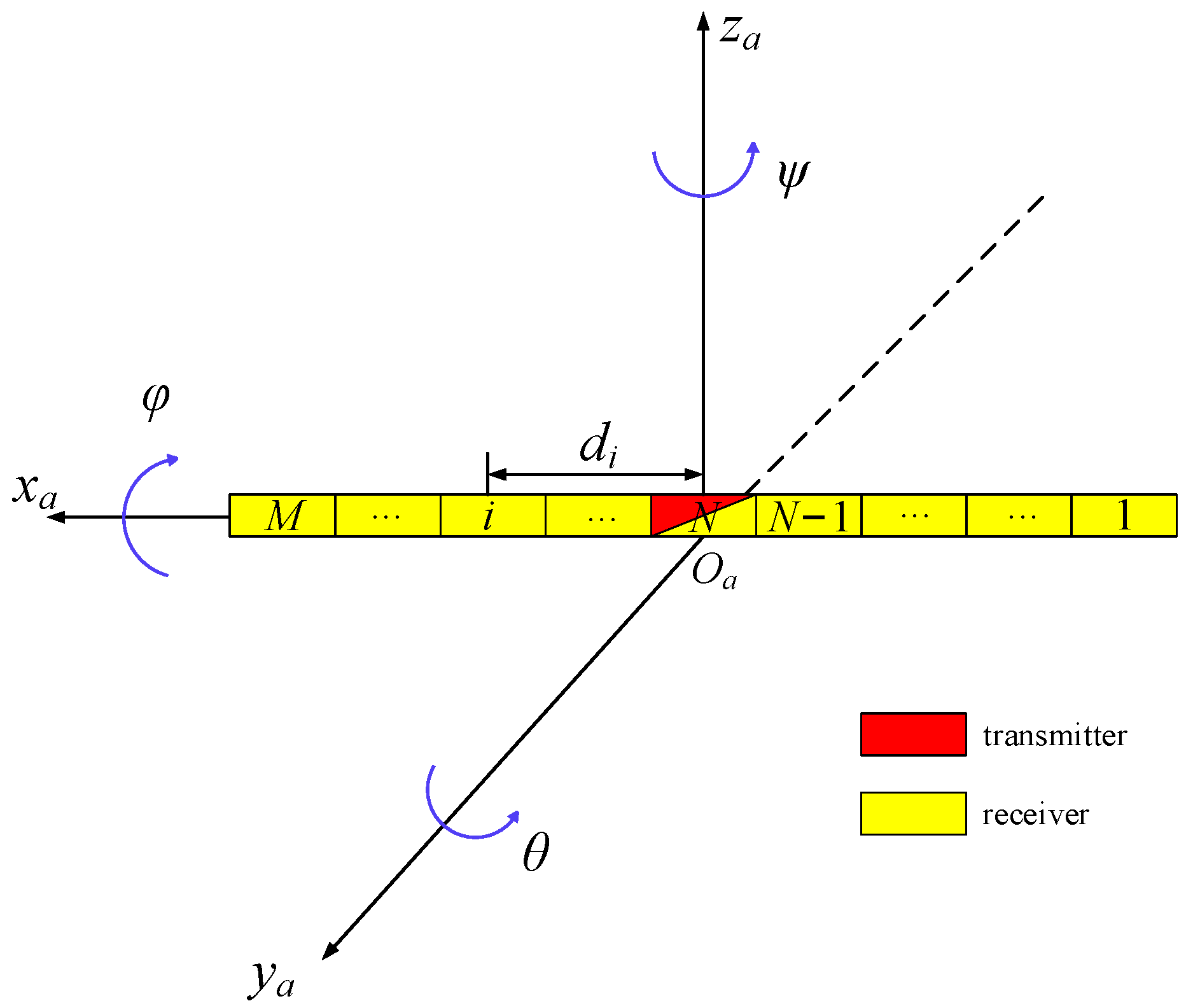
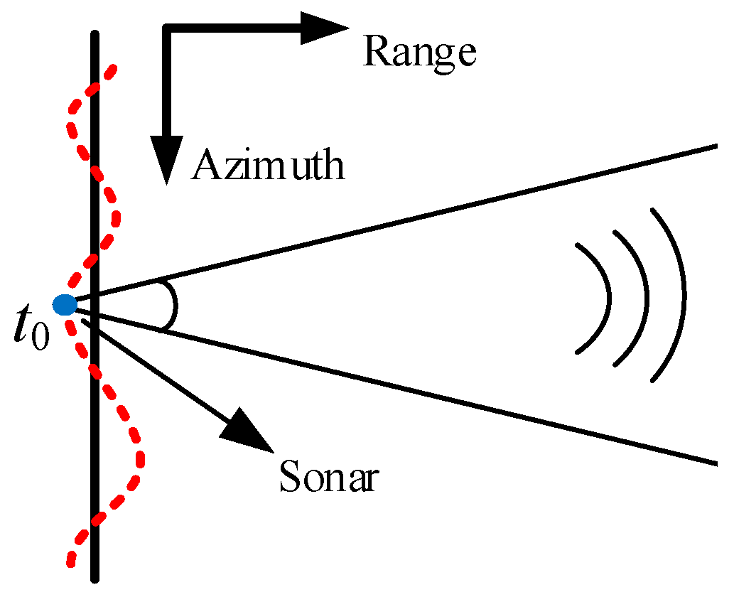
2. SAS Geometry and Exact Range History Error

The motion geometry of a multiple-receiver SAS is shown in Figure 1, and the nominal and actual trajectories of the SAS are shown as a blue line and red curve, respectively. We adjust the PRF and data recording speed using the X-axis velocity $V_A$ calculated by the accelerometer to ensure uniform along-track sampling. Assuming the ideal X-axis velocity and PRF are $V_{A0}$ and PRF₀, respectively, when the X-axis velocity changes to $V_A$, the corresponding PRF is adjusted to $V_A/V_{A0}\cdot {\mathrm{PRF}}_0$. Assuming that the surge has been fully compensated by a real-time adjustment of PRF, the azimuth sampling is uniform, and the equivalent velocity $V_A$ of the X-axis can be considered constant.

We suppose that there is a point target $P\left(0,r\cos E_s,-h\right)$ in the swath, where $r$ denotes the vertical slant range from the target to the nominal trajectory, $E_S$ denotes the target elevation angle, and $h$ denotes the height of the platform. The actual and ideal distances from the target to the transmitter are $R^{*}$ and $R$, respectively, and $H_M$ between the actual distance and the vertical slant range denotes the target azimuth angle.

The rectangular coordinate system $o_a{x}_a{y}_a{z}_a$ is established on the sonar array, as shown in Figure 2. The rotational center $O_a$ of the array coincides with the center of the transmitter. Please note that even when the rotational center deviates from the center of the transmitter, the rotational motion errors can also be converted into different combinations of the five-DOF motion errors in the coordinate system shown in Figure 2. To simplify the discussion, the motion errors discussed in this paper were converted into motion errors in the case that the rotational center coincides with the center of the transmitter. The rotational errors will cause not only the range history error of the multiple-receiver SAS but also the amplitude modulation of the signal [38]. However, because of the low requirement for beam directivity with wide-beam systems, the rotational errors usually do not exceed the maximum allowable directivity error, so amplitude modulation can be ignored [39], and only the range history error is considered.

We assume that $t$ is the azimuth slow time, and $\Delta y$ and $\Delta z$ are the sway and heave, respectively. When the transmitter moves to $\left(V_{A}t,\Delta y,\Delta z\right)$, the distance between the transmitter and the point target $P\left(0,r\cos E_s,-h\right)$ can be written as

$$R_T^{*}\left(t,r,\Delta y,\Delta z\right)=\sqrt{{\left(V_{A}t\right)}^2+{\left(\Delta y-r\cos E_S\right)}^2+{\left(\Delta z+h\right)}^2}.$$

(1)

We assume that ${\tau }_i^{*}$ is the signal propagation time between the signal transmitted from the transmitter and received by the receiver $i$ under the non-stop-hop-stop case, and motion errors remain unchanged during one pulse. Therefore, the coordinates of the receiver $i$ when receiving the signal are

$$\left[\begin{array}{c}{x}_i\\ y_i\\ z_i\end{array}\right]=\left[\begin{array}{c}{V}_{A}t+V_A{\tau }_i^{*}\\ \Delta y\\ \Delta z\end{array}\right]+M_{rotate}^{}\left[\begin{array}{c}{d}_i\\ 0\\ 0\end{array}\right]\begin{array}{c}\\ \\ .\end{array}$$

(2)

where $M_{rotate}^{}$ is the rotation matrix of the sonar array. In the coordinate system shown in Figure 2, according to the rotation sequence of yaw $\psi$, pitch $\theta$, and roll $\phi$, $M_{rotate}^{}$ can be expressed as

$$M_{rotate}^{}=\left[\begin{array}{c}\cos \psi \\ \sin \psi \\ 0\end{array}\begin{array}{c}-\sin \psi \\ \cos \psi \\ 0\end{array}\begin{array}{c}0\\ 0\\ 1\end{array}\right]\left[\begin{array}{c}\cos \theta \\ 0\\ -\sin \theta \end{array}\begin{array}{c}0\\ 1\\ 0\end{array}\begin{array}{c}\sin \theta \\ 0\\ \cos \theta \end{array}\right]\left[\begin{array}{c}1\\ 0\\ 0\end{array}\begin{array}{c}0\\ \cos \phi \\ \sin \phi \end{array}\begin{array}{c}0\\ -\sin \phi \\ \cos \phi \end{array}\right]$$

(3)

From (2) and (3), we obtain the coordinates of receiver $i$:

$$\left[\begin{array}{c}{x}_i\\ y_i\\ z_i\end{array}\right]=\left[\begin{array}{c}{V}_{A}t+V_A{\tau }_i^{*}+d_i\cos \theta \cos \psi \\ \Delta y+d_i\cos \theta \sin \psi \\ \Delta z-d_i\sin \theta \end{array}\right]\begin{array}{c}\\ \\ .\end{array}$$

(4)

It can be found that the roll $\phi$ is not included in (4), but this only indicates that the roll does not affect the range history of the signal in the coordinate system shown in Figure 2. However, since all the transmitters and receivers are mounted on the periphery of the platform, any roll component generates the $y$ and $z$ coordinates of the transmitters and the receiver. To simplify the discussion, the motion errors discussed in this paper were converted into motion errors in the coordinate system shown in Figure 2.

According to (4), the distance between the receiver $i$ and the point target $P\left(0,r\cos E_s,-h\right)$ is

$$R_{R,i}^{*}\left(t,r,\Delta y,\Delta z,\theta ,\psi \right)=\sqrt{{\left(V_{A}t+V_A{\tau }_i^{*}+d_i\cos \theta \cos \psi \right)}^2+{\left(\Delta y+d_i\cos \theta \sin \psi -r\cos E_S\right)}^2+{\left(\Delta z-d_i\sin \theta +h\right)}^2}.$$

(5)

The range history with motion errors is the sum of (1) and (5), and it can also be expressed as the product of sound velocity $c$ and the signal propagation time ${\tau }_i^{*}$. Therefore, the following equation can be listed:

$$R_T^{*}\left(t,r,\Delta y,\Delta z\right)+R_{R,i}^{*}\left(t,r,\Delta y,\Delta z,\theta ,\psi \right)=c{\tau }_i^{*}.$$

(6)

By solving (6), we have

$${\tau }_i^{*}=\frac{B_i^{*}+\sqrt{{\left(B_i^{*}\right)}^2+A{C}_i^{*}}}{A}$$

(7)

where

$$\left\{\begin{array}{l}A=c^2-V_A{}^2\\ B_i^{*}=V_A{d}_i\cos \theta \cos \psi +V_A{}^{2}t\\ \hspace{1em} +c\sqrt{V_A{}^2{t}^2+{\left(\Delta y-r\cos E_S\right)}^2+{\left(\Delta z+h\right)}^2}\\ C_i^{*}=2V_{A}t{d}_i\cos \theta \cos \psi +d_i{}^2-2d_i\sin \theta \left(\Delta z+h\right)\\ \hspace{1em} +2\left(\Delta y-r\cos E_S\right)d_i\cos \theta \sin \psi \end{array}\right.$$

(8)

Therefore, the range history with motion errors is

$$R_i^{*}\left(t,r,\Delta y,\Delta z,\theta ,\psi \right)=\frac{B_i^{*}+\sqrt{{\left(B_i^{*}\right)}^2+A{C}_i^{*}}}{A}c.$$

(9)

For convenience, the motion errors at time $t$ are expressed as $e_t$. For example, the range history $R_i^{*}\left(t,r,\Delta y,\Delta z,\theta ,\psi \right)$ in (9) can be rewritten as $R_i^{*}\left(t,r,e_t\right)$.

The range history without motion errors given in [40] is

$$R_i\left(t,r\right)=\frac{V_A{d}_i+V_A{}^{2}t+c\sqrt{V_A{}^2{t}^2+r^2}}{c^2-V_A{}^2}c+\frac{\sqrt{{\left(V_A{d}_i+V_A{}^{2}t+c\sqrt{V_A{}^2{t}^2+r^2}\right)}^2+\left(c^2-V_A{}^2\right)\cdot \left(2V_{A}t{d}_i+d_i{}^2\right)}}{c^2-V_A{}^2}c$$

(10)

According to (9) and (10), the exact range history error is

$$\begin{array}{l}\Delta R_i^{}\left(t,r,e_t\right)=R_i^{*}\left(t,r,e_t\right)-R_i\left(t,r\right)\\ =\frac{c}{c^2-V_A{}^2}\left\{V_A{d}_i\cos \theta \cos \psi +c\sqrt{V_A{}^2{t}^2+{\left(\Delta y-r\cos E_S\right)}^2+{\left(\Delta z+h\right)}^2}-V_A{d}_i\right.\\ -c\sqrt{V_A{}^2{t}^2+r^2}+\sqrt{{\left[V_A{d}_i\cos \theta \cos \psi +V_A{}^{2}t+c\sqrt{V_A{}^2{t}^2+{\left(\Delta y-r\cos E_S\right)}^2+{\left(\Delta z+h\right)}^2}\right]}^2}\\ \overline{+\left(c^2-V_A{}^2\right)\left[2V_{A}t{d}_i\cos \theta \cos \psi +d_i{}^2-2d_i\sin \theta \left(\Delta z+h\right)+2\left(\Delta y-r\cos E_S\right)d_i\cos \theta \sin \psi \right]}\\ \left.-\sqrt{{\left[V_A{d}_i+V_A{}^{2}t+c\sqrt{V_A{}^2{t}^2+r^2}\right]}^2+\left(c^2-V_A{}^2\right)\left(2V_{A}t{d}_i+d_i{}^2\right)}\right\}.\end{array}$$

(11)

Equation (11) shows that the range history error is a function of receiver $i$, range $r$, and azimuth $t$, so the receiver, azimuth, and range variation of the range history error should be considered simultaneously when compensating.

3. Analysis of Range History Error

The exact form of range history error is given in (11) above. The spatial-variant characteristics of range history errors with receivers $i$, range $r$, and azimuth time $t$ are the basis of the MOCO scheme, which will be analyzed in detail in this section.

3.1. Decomposition of Range History Error

The range history error is divided into two parts: the BCT and the RSVT. The BCT refers to the range history error on the beam centerline, which is the main part of the range history error and does not change with azimuth. The RSVT is the residual part of the range history error and is proportional to the cosine of the azimuth angle. The range history error after decomposition is expressed as

$$\begin{array}{l}\Delta R_i^{}\left(t,r,e_t\right)=\Delta R_{c,i}\left(-r/c-d_i/2v,r,e_t\right)+\Delta R_{v,i}\left(t,r,e_t\right)\\ \approx \Delta R_i^{}\left(-r/c-d_i/2v,r,e_t\right)+\Delta R_i^{}\left(-r/c-d_i/2v,r,e_t\right)\cdot \left(\cos H_M-1\right)\end{array}$$

(12)

where $\Delta R_i^{}\left(-r/c-d_i/2v,r,e_t\right)$ is the BCT, and $\Delta R_i^{}\left(-r/c-d_i/2v,r,e_t\right)\cdot \left(\cos H_M-1\right)$ is the RSVT. In (12), when the transmitter is located at the azimuth position $vt=-vr/c-d_i/2$, the signal is transmitted. At this time, the signal propagation time ${\tau }_i^{*}$ of the target with the coordinate $\left(0,r\right)$ is approximately $2r/c$, so the receiver will receive the signal at the azimuth position $vt+v{\tau }_i^{*}+d_i=vr/c+d_i/2$. Since the phase center of the transmitter and receiver is zero, the target can be considered to be located on the beam centerline. $t=-r/c-d_i/2v$ only means that the target is located at the beam centerline, but it does not mean that $e_t$ is the motion errors at $t=-r/c-d_i/2v$, while $e_t$ is still the motion errors at time $t$.

The typical BCT compensation methods include two-step MOCO [23] and one-step MOCO [24]. In the two-step MOCO, the range-variant phase error is compensated after range cell migration correction (RCMC), which would degrade the RCMC results [24]. Therefore, we use one-step MOCO to compensate for the time delay error and phase error caused by the BCT before RCMC. The time delay error and phase error caused by the BCT are compensated through interpolation and phase multiplication, respectively. The phase compensation function is

$$H_{mc,i}\left(r\right)=\exp \left[j\frac{2\pi }{\lambda }\Delta R_{c,i}\left(-r/c-d_i/2v,r,e_t\right)\right].$$

(13)

where $\lambda$ is the wavelength, and $\Delta R_{c,i}\left(-r/c-d_i/2v,r,e_t\right)$ is provided by (11).

Next, the received data during one pulse are treated as a subaperture along the azimuth direction. Using the correspondence between the target azimuth angle and Doppler frequency, the RSVT can be compensated in the subaperture azimuth-frequency domain. In the subaperture azimuth-frequency domain, since the receiver information cannot be distinguished, the RSVT of the reference receiver is used as compensation for all receivers, and (12) can be expressed as

$$\begin{array}{l}\Delta R_i^{}\left(t,r,e_t\right)=\Delta R_{c,i}\left(-r/c-d_i/2v,r,e_t\right)+\Delta R_{v,i}\left(t,r,e_t\right)\\ \approx \Delta R_i^{}\left(-r/c-d_i/2v,r,e_t\right)+\Delta R_{ref}^{}\left(-r/c-d_{ref}/2v,r,e_t\right)\cdot \left(\cos H_M-1\right)\\ =\Delta R_i^{}\left(-r/c-d_i/2v,r,e_t\right)+\Delta R_{ref}^{}\left(-r/c,r,e_t\right)\cdot \left(\cos H_M-1\right)\end{array}$$

(14)

where $ref$ represents the reference receiver. In this paper, the receiver located at the center of the subaperture ($d_{ref}=0$) is used as the reference receiver.

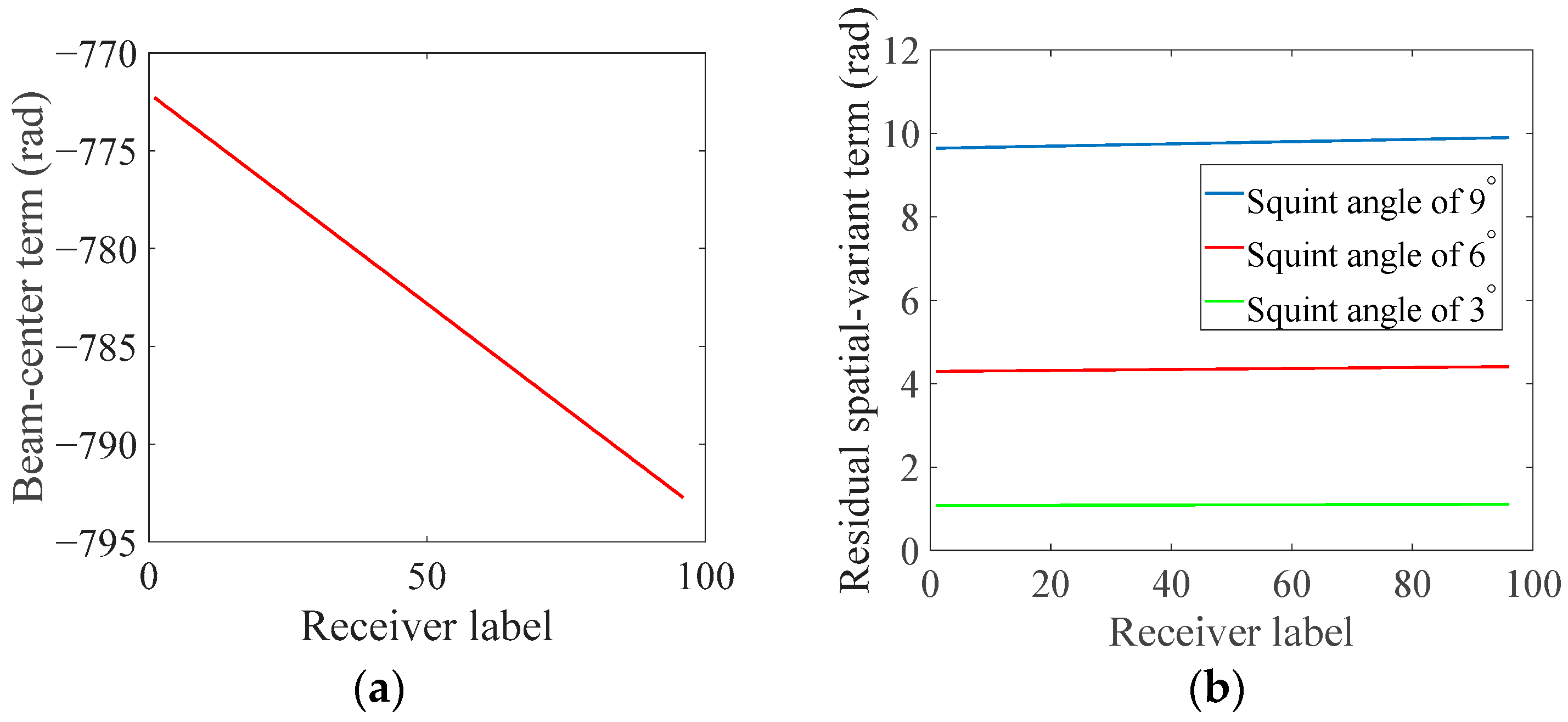
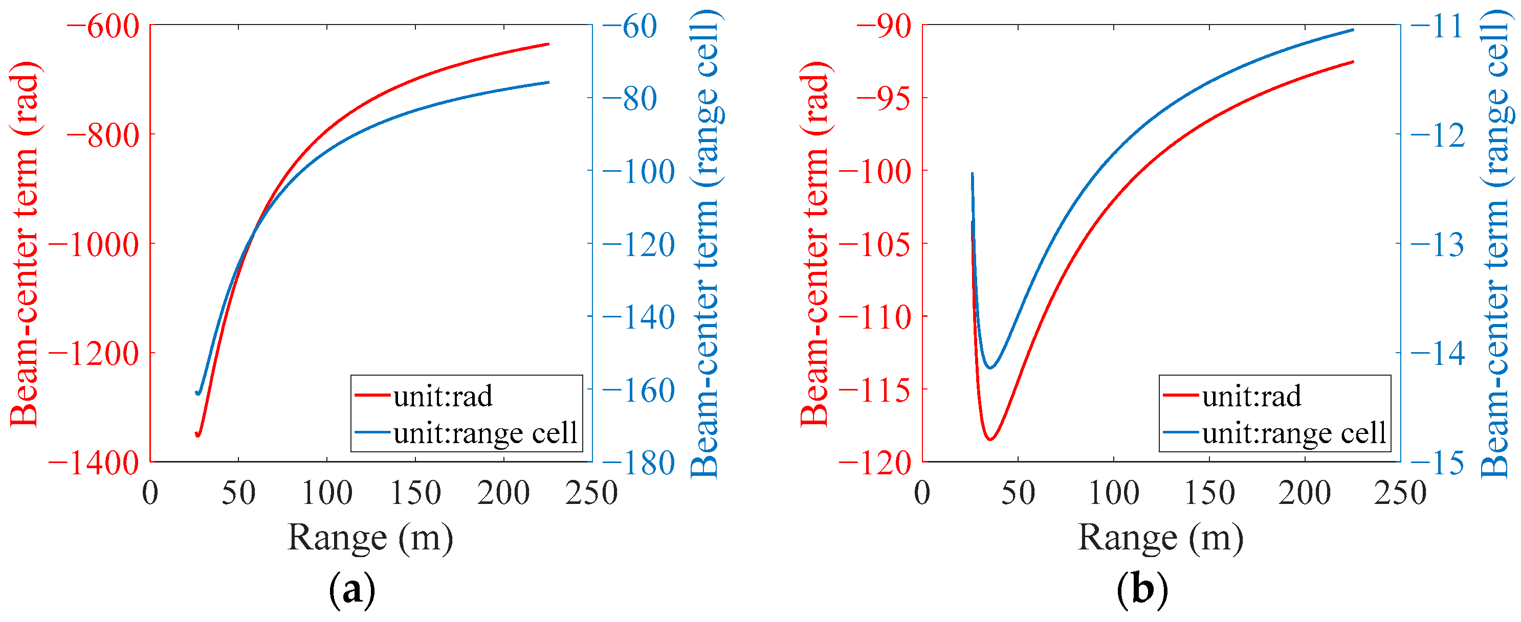
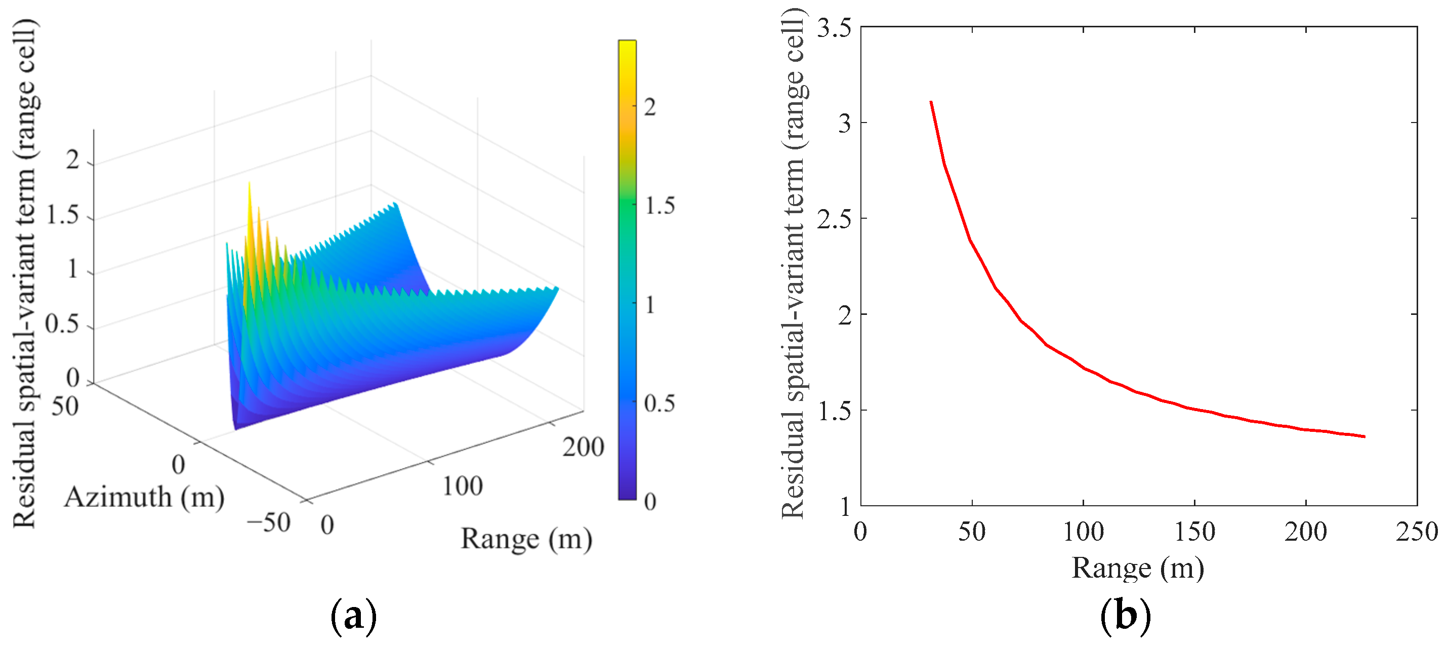
3.2. Spatial-Variant Characteristics of Range History Error

We analyze the spatial-variant characteristics of the BCT and RSVT in (14) through simulated data. Simulation experiments are conducted using typical parameters of the wide-beam HISAS 1030 system [41]. The system parameters are shown in

Table 1. Simulation parameters.

Parameter	Value	Parameter	Value
signal carrier frequency	100 kHz	length of transmitter	0.04 m
signal time width	20 ms	length of receiver	0.02 m
signal bandwidth	37.5 kHz	number of receivers	96
signal sampling frequency	56.25 kHz	platform velocity	3 m/s
pulse repetition interval	0.32 s	distance to the seabed	25 m

, with a horizontal beam width of 19°. The length of the receiver in Table 1 refers to the spacing between the receivers. To study the range history error characteristics of long-distance and long-array cases, the PRI and the number of receivers are appropriately increased.

The motion errors collected using the ChinSAS system of the Naval University of Engineering during a sea trial are used for simulation. The actual motion errors collected are shown in Figure 3.

As shown in Figure 4, the SAS system moves along the azimuth direction to collect data. The black solid line represents the ideal trajectory, and the red dashed line represents the actual motion trajectory. Without the loss of generality, the motion errors at time $t_0$ are set to the maximum value of motion errors in Figure 3; then, the sway, heave, yaw, and pitch are 0.6 m, 1.3 m, 1.2°, and 1.4°, respectively.

Assuming that the closest vertical slant distance between the target and SAS is 100 m, the variation curves of the BCT and RSVT with receivers are shown in Figure 5. It can be seen that the BCT changes rapidly with receivers, and the maximum difference of the BCT far exceeds $\pi /4$ radians, so each receiver must be compensated separately. The RSVT changes slowly with receivers but rapidly with the target’s squint angle. The difference between different squint angles of the same receiver far exceeds $\pi /4$ radians, while the maximum difference between receivers at the same squint angle is only about 0.26 radians, which is far less than the $\pi /4$ radians required for imaging. Therefore, when compensating for RSVTs with different squint angles, the RSVT of the reference receiver can be used to replace the RSVTs of other receivers.

Figure 5 shows the receiver dependence of the BCT and RSVT. Next, we continue to analyze the spatial-variant characteristics of the BCT and RSVT with range and azimuth. The edge receiver is affected by motion errors mostly, so we choose the edge receiver for analysis.

In the beam at time $t_0$ as shown in Figure 4, the BCT of the first receiver (edge receiver) is shown in Figure 6a. It can be seen that the variation range of the BCT in the entire swath far exceeds $\pi /4$ radians and a range cell. To fully show the changes in the BCT, the sway, heave, yaw, and pitch are reduced to 0.1 m, 0.1 m, 1°, and 1°, respectively. At this time, the BCT is shown in Figure 6b. It can be seen that the variation range of the BCT still exceeds $\pi /4$ radians and a range cell. Therefore, when compensating the BCT, the phase compensation function must be updated with range, and the RCM caused by the BCT is compensated by interpolation.

Figure 7a shows the RSVT of the first receiver (edge receiver), which can be found to be significantly azimuth-dependent. The RSVT at the beam edge in Figure 7a is shown in Figure 7b. It can be seen that the residual RCM caused by the RSVT exceeds one resolution cell, and its range dependency is significant, so it can be corrected by dividing the range into blocks to avoid the huge computation caused by interpolation.

In this section, we decompose the range history error into the BCT and RSVT and then simulate and analyze the spatial-variant characteristics of the range history error based on actual SAS system parameters and motion errors. The compensation of the BCT is similar to that of wide-beam SAR systems. However, because of the large ratio of swath width to the range in the wide swath, the wide beam, and high range resolution, it is necessary to consider the 2D spatial-variant characteristics of the residual RCM caused by the RSVT during compensation, which has not been considered in existing algorithms.

4. Subaperture MOCO Algorithm

Based on the 2D spatial-variant characteristics of the range history error discussed in Section 3, we propose a two-stage compensation scheme.

The first stage mainly compensates the BCT. We adopt a one-step MOCO to comprehensively correct the time delay and phase error of the BCT after range compression and before RCMC. The second stage mainly compensates the RSVT. After dividing the data into a series of subapertures along the azimuth-time domain, the corresponding relationship between Doppler frequency and the target azimuth angle is used to compensate for the RSVT in the azimuth-frequency domain. Considering the 2D spatial-variant characteristics of residual RCM caused by the RSVT, the range block compensation is performed. Figure 8 shows the detailed flow of the proposed MOCO algorithm.

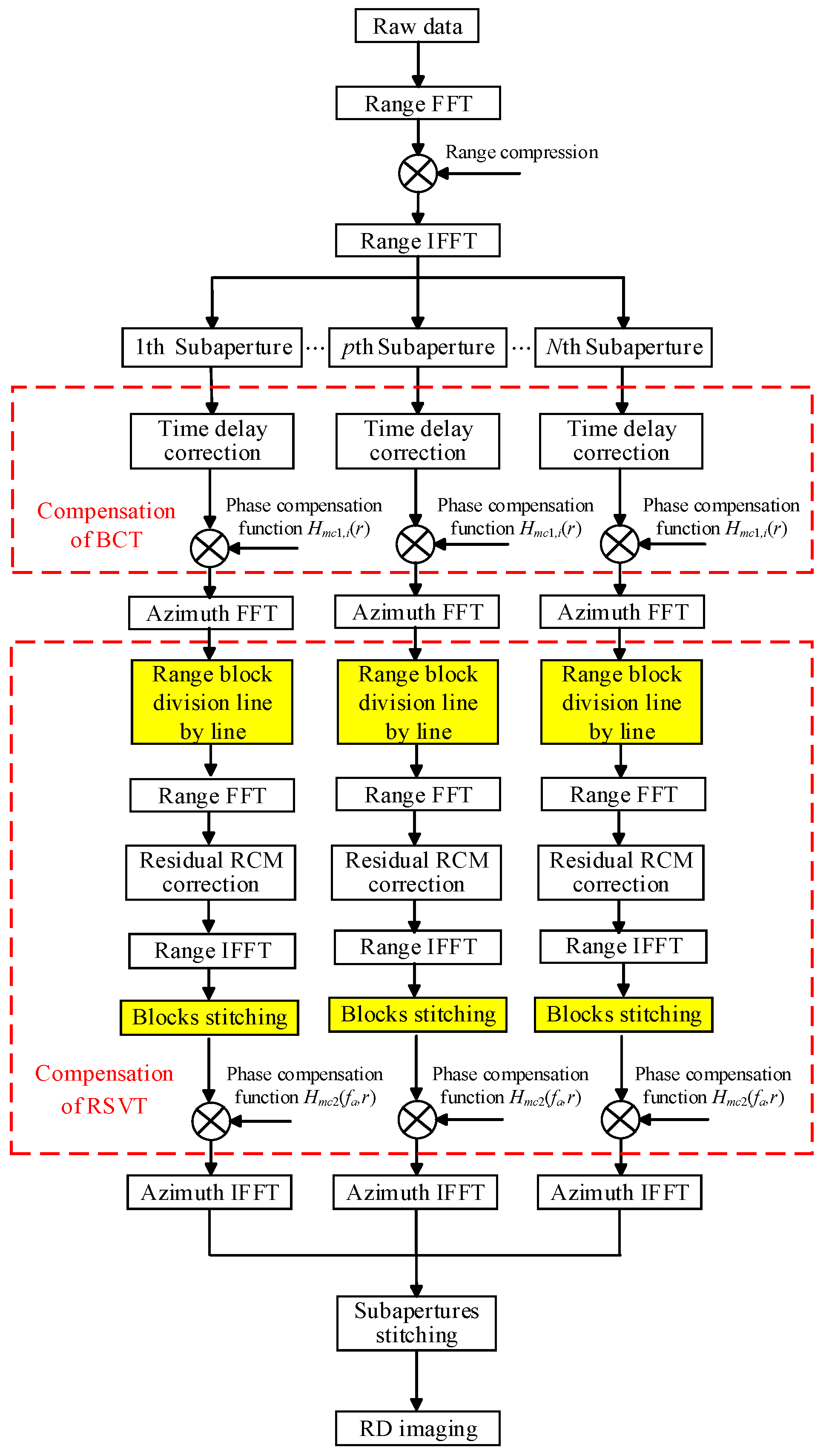
4.1. Algorithm Process

4.1.1. Compensation of BCT

The baseband signal in the 2D time domain can be expressed as

$$\begin{array}{l}ss\left(\tau ,t,r\right)=A{\omega }_r\left[\tau -\frac{R_i^{*}\left(t,r,e_t\right)}{c}\right]{\omega }_a\left(t\right)\\ \exp \left[-j\frac{2\pi R_i^{*}\left(t,r,e_t\right)}{\lambda }\right]\exp \left\{j\pi K_r{\left[\tau -\frac{R_i^{*}\left(t,r,e_t\right)}{c}\right]}^2\right\}\end{array}$$

(15)

where $A$ is the signal amplitude, ${\omega }_r\left(\tau \right)$ is the pulse envelope, $\tau$ is the range fast time, ${\omega }_a\left(t\right)$ is the beam pattern determined by the receiver $i$ and the transmitter, $R_i^{*}\left(t,r,e_t\right)$ is the range history with the motion errors, $\lambda$ is the wavelength, and $K_r$ is the signal frequency modulation slope. To simplify the analysis, the amplitude independent of the imaging quality is ignored in the subsequent derivation.

After the range compression, the compressed signal in the 2D time domain is expressed as

$$\begin{array}{l}ss\left(\tau ,t,r\right)=\sin c\left\{B_r\left[\tau -\frac{R_i\left(t,r\right)}{c}-\frac{\Delta R_{c,i}\left(-r/c-d_i/2v,r,e_t\right)+\Delta R_{v,i}\left(t,r,e_t\right)}{c}\right]\right\}\\ {\omega }_a\left(t\right)\exp \left\{-j\frac{2\pi }{\lambda }\left[R_i\left(t,r\right)+\Delta R_{c,i}\left(-r/c-d_i/2v,r,e_t\right)+\Delta R_{v,i}\left(t,r,e_t\right)\right]\right\}\end{array}$$

(16)

where $B_r$ is the range bandwidth. After interpolation compensation for the RCM caused by $\Delta R_{c,i}\left(-r/c-d_i/2v,r,e_t\right)$, (16) becomes

$$\begin{array}{l}ss\left(\tau ,t,r\right)=\sin c\left\{B_r\left[\tau -\frac{R_i\left(t,r\right)}{c}-\frac{\Delta R_{v,i}\left(t,r,e_t\right)}{c}\right]\right\}\\ {\omega }_a\left(t\right)\exp \left\{-j\frac{2\pi }{\lambda }\left[R_i\left(t,r\right)+\Delta R_{c,i}\left(-r/c-d_i/2v,r,e_t\right)+\Delta R_{v,i}\left(t,r,e_t\right)\right]\right\}\end{array}$$

(17)

Then, we compensate the phase error caused by the BCT. The phase compensation function is

$$H_{mc1,i}\left(r\right)=\exp \left[j\frac{2\pi }{\lambda }\Delta R_{c,i}\left(-r/c-d_i/2v,r,e_t\right)\right].$$

(18)

The signal after phase compensation can be expressed as

$$\begin{array}{l}ss\left(\tau ,t,r\right)=\sin c\left\{B_r\left[\tau -\frac{R_i\left(t,r\right)}{c}-\frac{\Delta R_{v,i}\left(t,r,e_t\right)}{c}\right]\right\}{\omega }_a\left(t\right)\\ \exp \left[-j\frac{2\pi }{\lambda }{R}_i\left(t,r\right)\right]\exp \left[-j\frac{2\pi }{\lambda }\Delta R_{v,i}\left(t,r,e_t\right)\right].\end{array}$$

(19)

Only the range history error of the beam center is accurately compensated after the compensation of the BCT. In the second stage, the RSVT will be compensated.

4.1.2. Compensation of RSVT

Next, we compensate the RSVT $\Delta R_{v,i}\left(t,r,e_t\right)$ in (19). We take the received data during one pulse as a subaperture and perform the azimuth FFT in the subaperture to enter the RD domain. Then, the residual RCM and phase error caused by the RSVT are sequentially compensated.

As shown in Figure 7a above, the RSVT is highly azimuth-dependent, so it is necessary to compensate line-by-line (range direction) in the subaperture azimuth-frequency domain. The yellow box steps in Figure 8 represent the block correction of the residual RCM. After the residual RCM correction is completed, the phase error is compensated in the subaperture RD domain, and the phase error compensation function is

$$H_{mc2}\left(f_a,r\right)=\exp \left[j\frac{2\pi }{\lambda }\Delta R_{ref}^{}\left(-r/c,r,e_t\right)\cdot \left(\cos H_M-1\right)\right]$$

(20)

where $f_a$ is the azimuth frequency, $\Delta R_{ref}^{}\left(-r/c,r,e_t\right)$ is obtained by making $t=-r/c$ in (11), and $H_M$ is obtained by $f_a=2V_A\sin H_M/\lambda$.

It should be noted that the phase compensation is performed before the RCMC of the RD algorithm. Therefore, when the azimuth frequency is not zero in the subaperture RD domain, the true vertical distance of the target is not $r$, but $r\cos H_M$, where $H_M$ is the azimuth angle. Substituting this $r$ as the vertical distance into (20) will introduce an error, but Figure 7b shows that this error caused by RCM can be completely ignored.

The signal after phase compensation is processed with an azimuth inverse FFT (IFFT) in the subaperture, and then subapertures are stitched along the azimuth without overlapping. The resulting signal can be expressed as

$$ss\left(\tau ,t,r\right)=\sin c\left\{B_r\left[\tau -\frac{R_i\left(t,r\right)}{c}\right]\right\}{\omega }_a\left(t\right)\exp \left[-j\frac{2\pi R_i\left(t,r\right)}{\lambda }\right].$$

(21)

After the above compensation steps, the range history error is essentially compensated, but there is still a residual phase error. In Section 5.1, we analyze the residual phase error through simulated data. Generally, the residual phase error fulfills the imaging requirements of less than one-eighth of the wavelength.

4.1.3. Imaging

After BCT compensation and RSVT compensation, the SAS data are compensated as ideal data without motion errors. Next, the method in [36] is adopted to convert the data of a multiple-receiver SAS into the monostatic SAS equivalents, and then the monostatic RD algorithm [37] is used for imaging.

4.2. Applicable Conditions of the Algorithm

The proposed algorithm employs an azimuth-time domain subaperture method to accurately compensate the RSVT of the range history error. We treat the received data of each pulse as a subaperture and compensate the residual RCM and phase error caused by the RSVT in the subaperture azimuth-frequency domain. In fact, the subaperture size is a compromise between trajectory deviation accommodation and angle accommodation. In this section, we will discuss the applicable conditions for using single-pulse data as subaperture processing.

Compensating the approximate range history error of (14) as the exact range history error of (11) will introduce an additional error, which we call the reference receiver approximation error. The reference receiver approximation error ${\delta }_{e,ref}$ can be obtained by subtracting (14) from (11)

$${\delta }_{e,ref}=\left|\Delta R_i^{}\left(t,r,e_t\right)-\Delta R_i^{}\left(-r/c-d_i/2v,r,e_t\right)-\Delta R_{ref}^{}\left(-r/c,r,e_t\right)\cdot \left(\cos H_M-1\right)\right|$$

(22)

On the other hand, the size of the subaperture determines the frequency interval and angle accommodation, and the error related to the angle accommodation is referred to as the angle accommodation error ${\delta }_{e,angle}$. The error is zero when the target azimuth is located at the center of the angle interval, and the error is maximum when the target azimuth is located at the edge of the angle interval. The maximum value of the error is expressed as

$${\delta }_{e,angle}=\left|\Delta R_{ref}^{}\left(-r/c,r,e_t\right)\cdot \left[\cos H_M-\cos \left(H_M-{\delta }_{H_M}/2\right)\right]\right|$$

(23)

where ${\delta }_{H_M}$ is the angular resolution of the subaperture. To ensure imaging quality, the reference receiver approximation error and angle accommodation error should meet

$${\delta }_{e,ref}+{\delta }_{e,angle}<\frac{\lambda }{8}$$

(24)

These two errors are discussed separately below.

4.2.1. Reference Receiver Approximation Error

The establishment of (23) is a strict condition for meeting imaging requirements. For convenient analysis of the reference receiver approximation error and angle accommodation error, a necessary condition for satisfying imaging requirements is that these two errors are less than one-eighth of the wavelength each. Therefore, the reference receiver approximation error satisfies

$${\delta }_{e,ref}<\frac{\lambda }{8}$$

(25)

By substituting (12) into (22), the condition of (25) can be relaxed to

$${\delta }_{e,ref}=\left|\left[\Delta R_i^{}\left(-r/c-d_i/2v,r,e_t\right)-\Delta R_{ref}^{}\left(-r/c,r,e_t\right)\right]\cdot \left(\cos H_M-1\right)\right|<\frac{\lambda }{8}$$

(26)

when the azimuth angle $H_M$ takes the maximum value $H_{M,\max }=\lambda /\left(2D_T\right)$, ${\delta }_{e,ref}$ is the maximum, where $D_T$ is the length of the transmitter, and then (26) can be re-expressed as

$$\left|\left[\Delta R_i^{}\left(-r/c-d_i/2v,r,e_t\right)-\Delta R_{ref}^{}\left(-r/c,r,e_t\right)\right]\right|<\frac{\lambda }{8}\cdot \frac{1}{1-\sqrt{1-\frac{{\lambda }^2}{4D_T^2}}}$$

(27)

where $\Delta R_i^{}\left(-r/c-d_i/2v,r,e_t\right)$ and $\Delta R_{ref}^{}\left(-r/c,r,e_t\right)$ are the BCTs of the receiver $i$ and the reference receiver, respectively. Equation (27) gives an upper limit for the difference between the BCTs of different receivers and the reference receiver, which is only related to the wavelength and the transmitter length. Obviously, the farther the receiver $i$ is from the reference receiver, the greater the left value in (27). Therefore, satisfying (27) for an edge receiver is a necessary condition for allowing the processing of single-pulse data as a subaperture.

4.2.2. Angle Accommodation Error

Make the angle accommodation error meet the requirement

$${\delta }_{e,ref}=\left|\Delta R_{ref}^{}\left(-r/c,r,e_t\right)\cdot \left[\cos H_M-\cos \left(H_M-{\delta }_{H_M}/2\right)\right]\right|<\frac{\lambda }{8}$$

(28)

Obtained by deformation of (28)

$$\left|\Delta R_{ref}^{}\left(-r/c,r,e_t\right)\right|<\frac{\lambda }{8\left|\cos H_M-\cos \left(H_M-{\delta }_{H_M}/2\right)\right|}$$

(29)

where $\Delta R_{ref}^{}\left(-r/c,r,e_t\right)$ is the BCT of the range history error of the reference receiver. With the beam width less than 90°, the right side of (29) has a minimum value when the azimuth angle $H_M$ is taken as the maximum value $H_{M,\max }=\lambda /\left(2D_T\right)$. The relationship between subaperture angular resolution ${\delta }_{H_M}$ and the subaperture frequency interval $\Delta f$ is as follows:

$$\frac{2v}{\lambda }{\delta }_{H_M}=\Delta f$$

(30)

When the azimuth displacement of the SAS within a pulse is half the array length, the frequency interval within the subaperture is the PRF. According to (30), it can be deduced that the angular resolution is

$${\delta }_{H_M}=\frac{\mathrm{PRF}\cdot \lambda }{2v}=\frac{\lambda }{L_s}$$

(31)

where $L_s$ is the array length. Substitute (30) and $H_{M,\max }=\lambda /\left(2D_T\right)$ into (28) to obtain

$$\left|\Delta R_{ref}^{}\left(-r/c,r,e_t\right)\right|<\frac{\lambda }{8\left|\cos \left(\lambda /2D_T\right)-\cos \left[\left(\lambda /2D_T\right)-\left(\lambda /2L_s\right)\right]\right|}$$

(32)

The above equation gives the condition that needs to be satisfied for the BCT of the reference receiver, which is considered in terms of angle accommodation. The right side of (32) is a monotonically increasing function of the array length. The smaller the array length, the stricter the restriction on the BCT of the reference receiver.

Equation (24) gives the strict conditions that should be satisfied for the reference receiver approximation error and the angle accommodation error. To facilitate analysis, we discuss the loose conditions that should be satisfied for these two errors, as shown in (27) and (32). Equation (27) defines the upper limit of the subaperture size and (32) defines the lower limit of the subaperture size. Meeting these two restrictions on the array length is a necessary condition for processing single-pulse data as a subaperture. This processing method is satisfactory under normal motion errors. For example, under the system parameters shown in Table 1, the maximum allowable rotation error in the line of sight (LOS) given by (26) is 6.2°, and the maximum allowable translational error in the LOS given by (31) is 2.6 m, while the actual motion errors usually do not reach these magnitudes.

In addition, the derivation of the range history error of the algorithm in this paper is terrain-independent, so the performance of the algorithm may be degraded under severe terrain fluctuations.

4.3. Computational Efficiency

We analyze the computational efficiency of the algorithm from FFT and interpolation operations. Assume that the data size is $N_a\times N_r$, where $N_a$ is the azimuth data amount, and $N_r$ is the range data amount. In the first stage of compensation, the calculation time is mainly used for tedious interpolation operations. In the second stage of compensation, each subaperture mainly includes one azimuth FFT and IFFT operation, as well as several FFT and IFFT operations within several range blocks. Therefore, the total calculation amount in the second stage is approximately

$$O(\cdot )=N_a\cdot N_r\cdot {\log }_2{N}_s+N_a\cdot N_r\cdot {\log }_2{N}_b$$

(33)

where $N_s$ is the azimuth subaperture size, and $N_b$ is the range block size. Compared with the classical SATA algorithm, interpolation compensation for RCM caused by the BCT and range block correction for residual RCM caused by the RSVT are the main reasons for the increased computational complexity of this algorithm. In the actual compensation process, the residual RCM caused by the RSVT needs to be corrected when it is greater than 0.5 resolution cells, so the calculation amount is only moderately increased compared with the SATA algorithm.

5. Experiments and Results

In this section, we compare the compensation performance of the algorithm in [18], the SATA algorithm, and the proposed algorithm in this paper through simulated and real-data experiments, verifying the effectiveness of the proposed algorithm. In the simulation experiment, the residual phase errors of the three algorithms after compensation are compared, and then the imaging results of the three algorithms are compared under different distributed motion errors. In the real-data experiment, the imaging results of the three algorithms are compared through the data collected using the ChinSAS system to verify the effectiveness of the algorithm in this paper. After compensation, the same wide-beam RD algorithm is used for imaging, and there is no weighting processing in both range and azimuth.

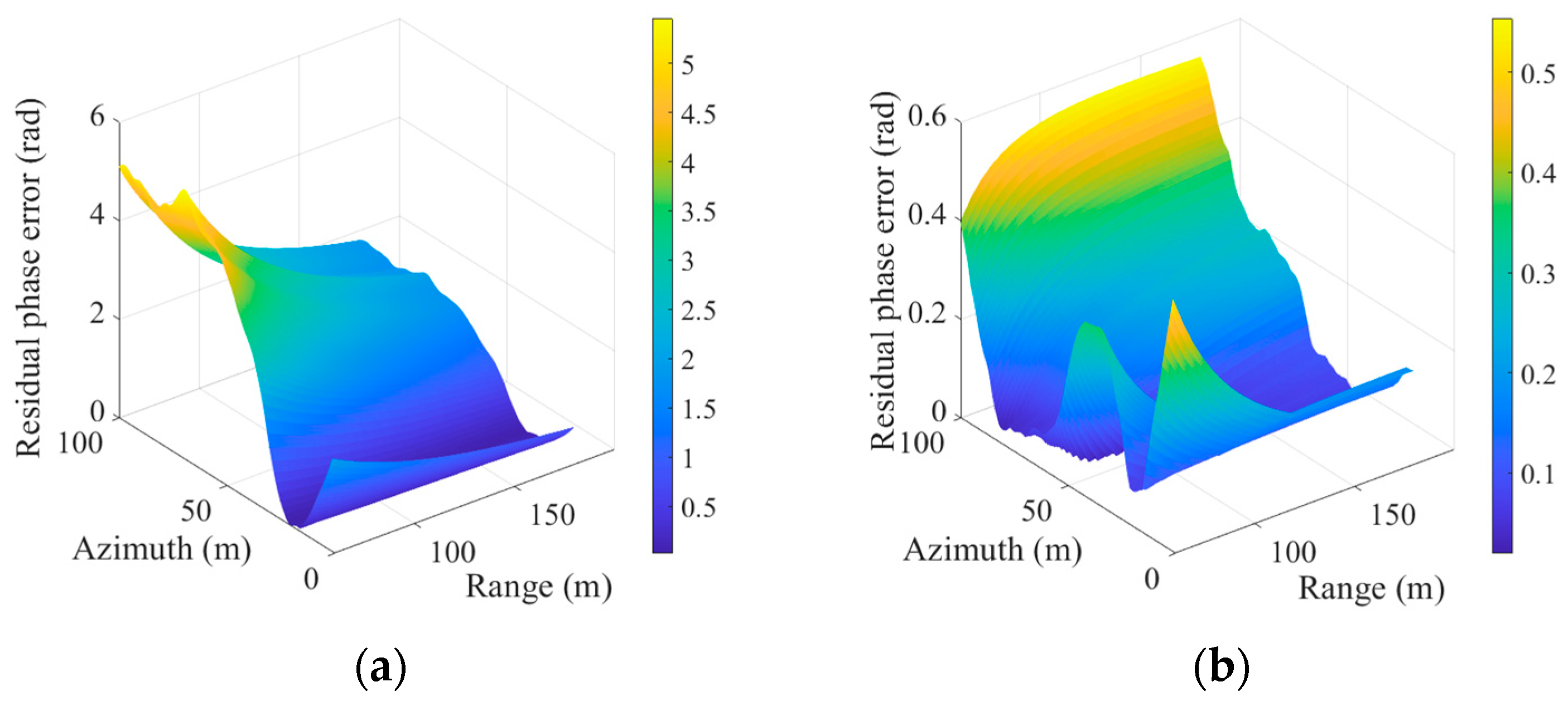
5.1. Residual Phase Error

After compensation by the three algorithms, there is still residual phase error, mainly including reference receiver approximation error and angle accommodation error. After compensation, the sum of these two errors should be less than one-eighth of the wavelength. Since the algorithm in [18] ignores the impact of heave and pitch on MOCO, the resulting residual phase error is much greater than the SATA algorithm and proposed algorithm, so only the residual phase errors of the SATA algorithm and the algorithm in this paper are shown.

The typical parameters of the HISAS 1030 system in Table 1 are used for simulation. The near and far ranges of the mapping zone are 75 m and 165 m, respectively. The horizontal beam width is 19° approximately. The motion errors are collected using the ChinSAS system of the Naval University of Engineering during a sea trial, as shown in Figure 3 above. Without losing generality, the first receiver (edge receiver) is selected for analysis. Figure 9 shows the residual phase error at the beam edge of this receiver.

As can be seen from Figure 9a, the residual phase error of the SATA algorithm mostly exceeds the required criteria for imaging, which may seriously affect imaging quality. The residual phase error of the proposed algorithm in Figure 9b is much smaller than that of the SATA algorithm and less than $\pi /4$, which can better meet the imaging requirements, demonstrating the advantages of the algorithm in this paper.

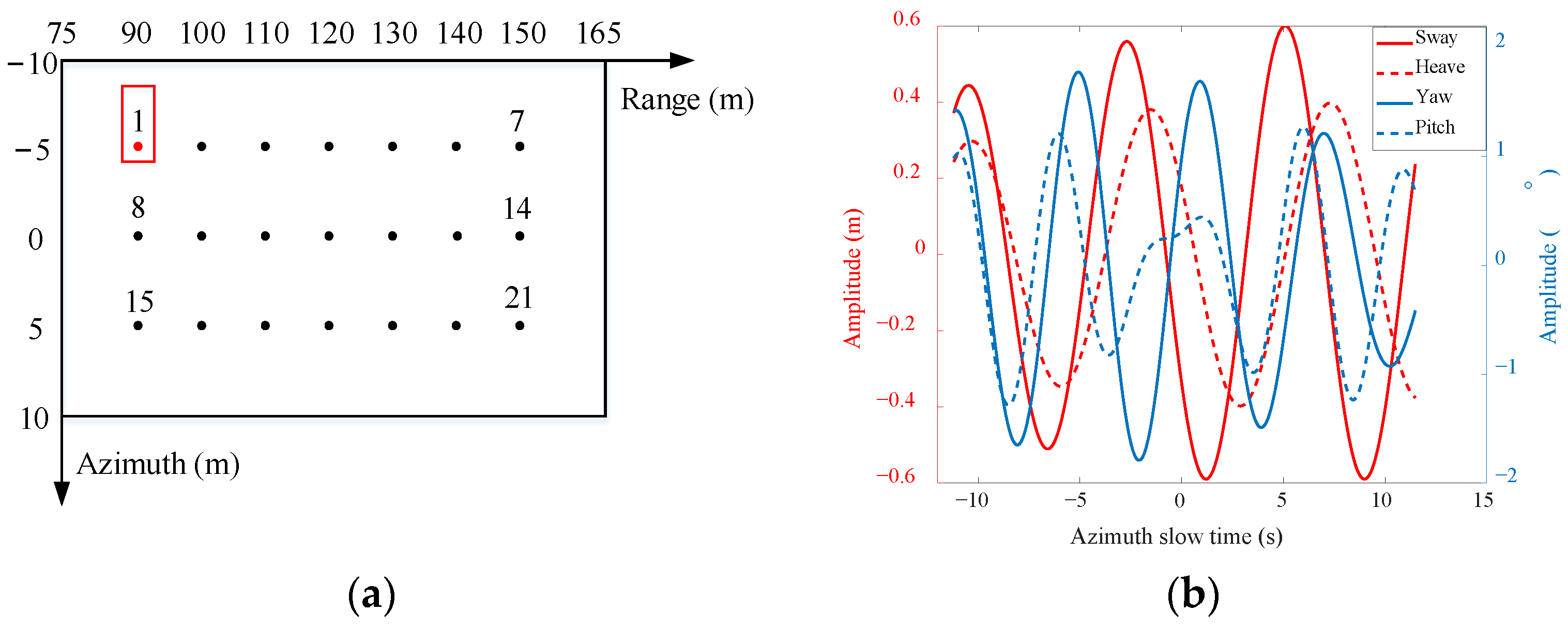
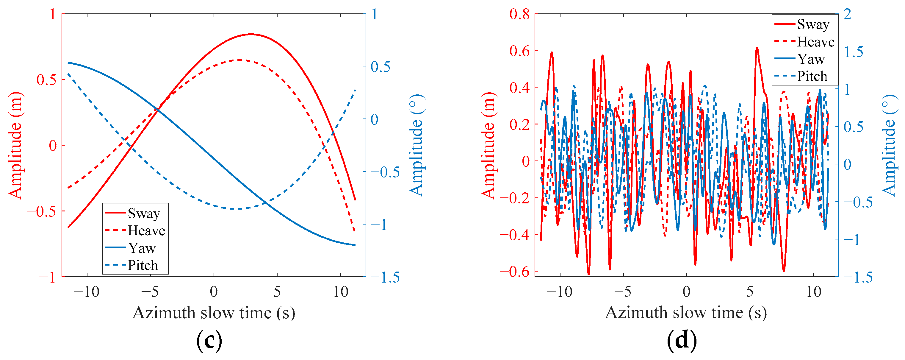
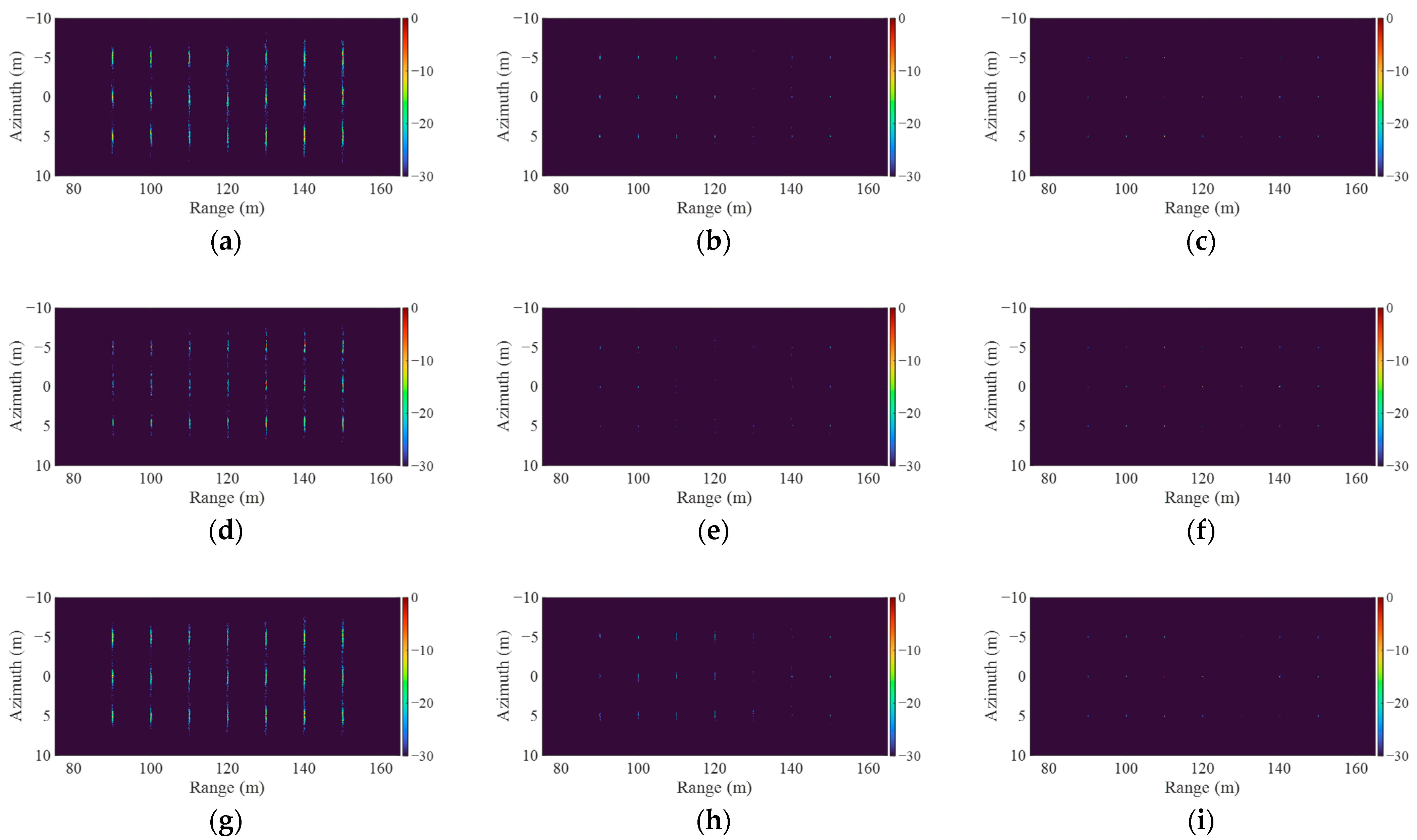
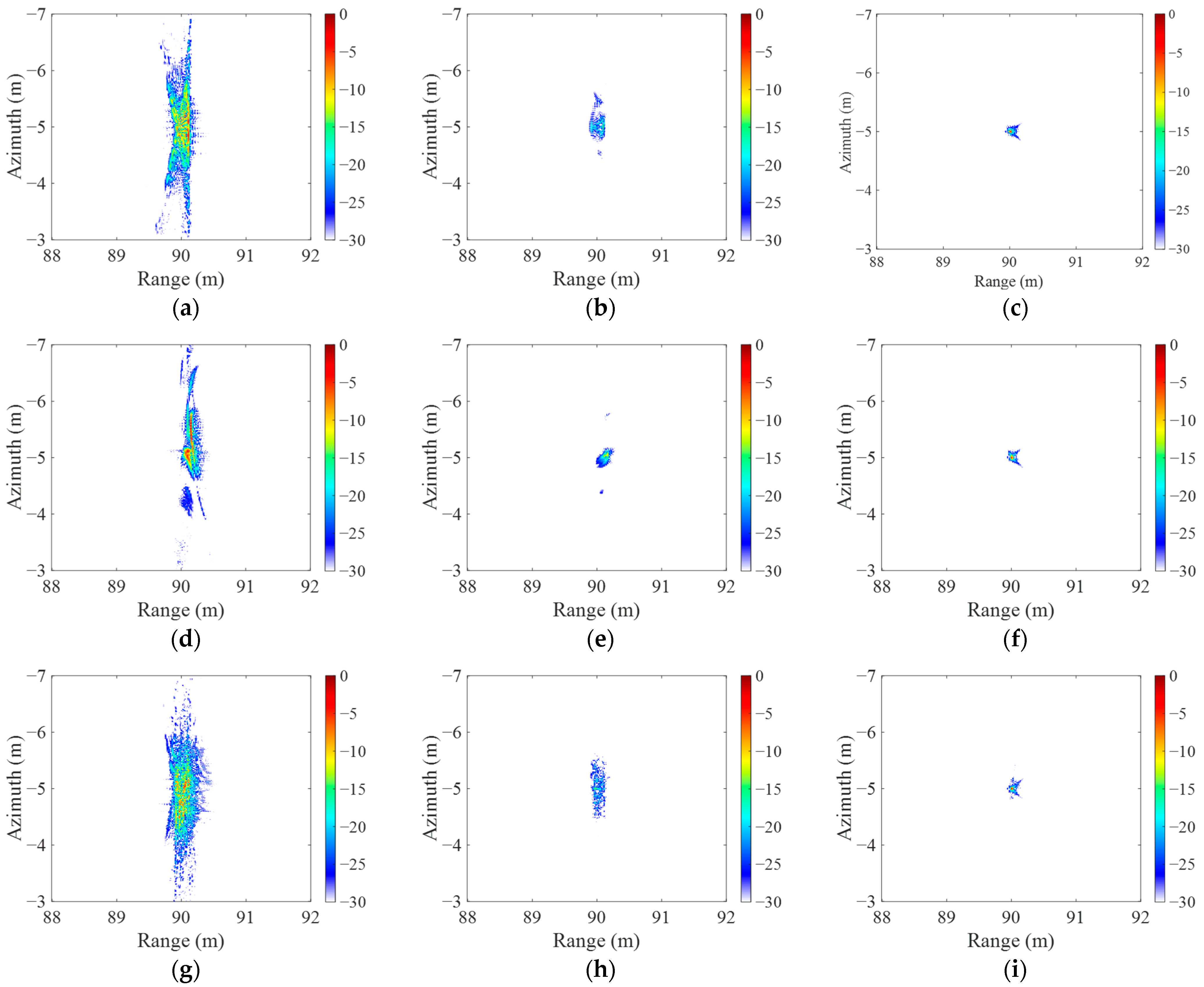
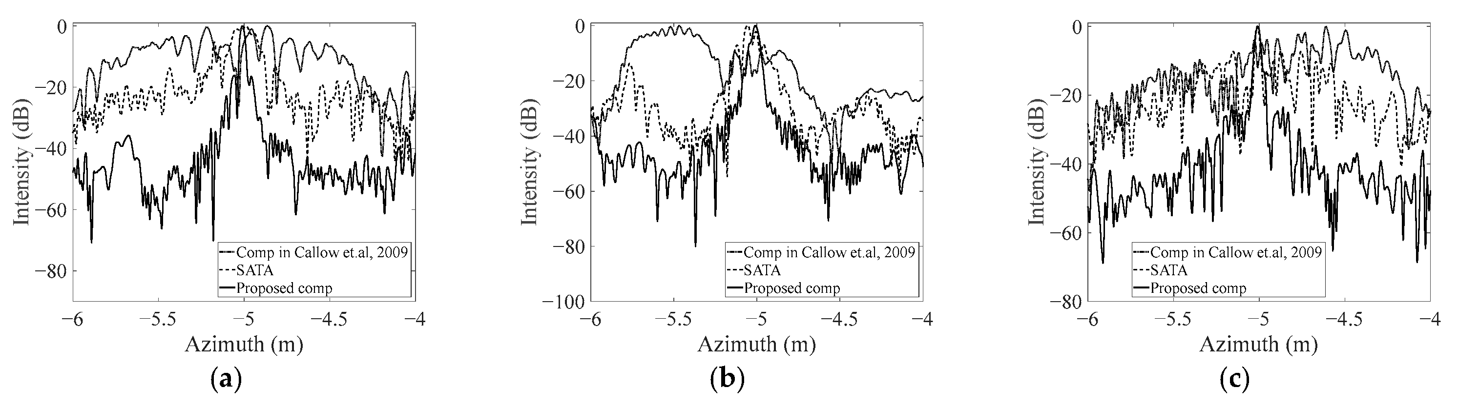
5.2. Ideal Point Target Imaging

In this section, we compare the compensation performance of the algorithms in [18], the SATA algorithm, and the proposed algorithm through ideal point target imaging under sinusoidal motion errors, cubic polynomial motion errors, and uniform random motion errors, respectively. The computing operating system is Microsoft Windows 11 (64 bit), the CPU is a quad-core Intel (R) Core (TM) i5-1135G7@2.42GHz, the memory is 16 GB, and the MATLAB version is R2021a. Typical parameters of the HISAS 1030 system are shown in Table 1.

The targets in the swath are shown in Figure 10a and are located on three horizontal lines with the azimuth coordinates of −5 m, 0 m, and 5 m, respectively. The labels of targets are shown in the figure. Target 1 (shown in the red box) is chosen for profile and parameter analysis in the following text. To ensure that the farthest target experiences a complete synthetic aperture length, the number of pulses is set to 72, and the corresponding azimuth coordinates are −34.5 m to 34.5 m. For display convenience, the azimuth coordinates in Figure 10a and the following figures only show −10 m to 10 m. The sinusoidal errors, cubic polynomial errors, and uniform random errors are shown in Figure 10, whose magnitude is similar to the collected motion errors in Figure 3.

Figure 11 shows the imaging results of ideal point targets using the [18] algorithm, the SATA algorithm, and the proposed algorithm under different distributed motion errors. Overall, the compensation effect of the algorithm in [18] is always the worst, with severe azimuth defocus, resulting in a large number of ghost targets. The compensation performance of the SATA algorithm is slightly better than that of [18], but there is still a relatively serious defocus. Compared with the previous two algorithms, the compensation performance of the algorithm in this paper is the best, and the azimuth focus is better. The compensation performance of the proposed algorithm does not significantly decrease under three different distributed motion errors and exhibits strong robustness. Without losing generality, target 1 is chosen to specifically analyze in the following text.

Figure 12 shows the local imaging results of target 1 under different distributed motion errors using the three compensation algorithms. It can be seen that under different distributed motion errors, the target response area of the algorithm in [18] is always the largest (especially along the azimuth), followed by the SATA algorithm, and the algorithm in this paper is always the smallest. The algorithm in this paper exhibits good compensation performance under different distributed motion errors, reflecting the effectiveness and robustness of the proposed algorithm.

Figure 13 shows the azimuth profiles of target 1 after compensation by three algorithms. It can be seen that under different distributed motion errors, the compensation performance of the algorithm in [18] is always poor, and it is essentially unable to focus effectively. This shows that although the azimuthal variability of motion errors is considered in [18], the error caused by heave and pitch and the residual 2D spatial-variant RCM is still serious. Compared with the algorithm in [18], the compensation performance of the SATA algorithm improved significantly, but the main lobe is still wide, and multiple peaks can easily be considered as ghost targets, with the maximum sidelobe approaching −5 dB. Compared with the previous two algorithms, the advantages of this algorithm are obvious, with a narrower main lobe width and a minimum sidelobe of less than −20 dB. The proposed algorithm exhibits good compensation performance and robustness under different motion errors.

To quantitatively analyze the compensation performance of the three compensation algorithms, we compare the compensation results of different algorithms through the impulse response width (IRW), peak sidelobe level ratio (PSLR), and integrated sidelobe level ratio (ISLR) of the azimuth profiles. In Figure 13, the azimuth profiles of the compensation in [18] are the worst, so only the parameters of the SATA algorithm and the algorithm in this paper are given, as shown in

Table 2. Parameters after compensation.

Motion Errors	Algorithm	IRW (cm)	PSLR (dB)	ISLR (dB)	Time (s)
Sinusoidal	Proposed algorithm	3.07	−16.24	−13.05	28.64
	SATA	14.45	−5.66	−7.48	16.62
Cubic polynomial	Proposed algorithm	3.95	−17.29	−18.66	28.94
	SATA	8.01	−6.75	−4.65	16.45
Uniform random	Proposed algorithm	3.18	−22.98	−16.50	30.93
	SATA	2.50	−7.33	2.99	16.52

. Overall, the parameters of the proposed algorithm are essentially superior to those of the SATA algorithm. The PSLR and ISLR of the proposed algorithm are always much lower than those of the SATA algorithm. Although the IRW of the SATA algorithm under uniform random motion errors is better than that of the proposed algorithm, the corresponding PSLR is as high as −7.33 dB, and the ISLR is a positive value. In terms of computational efficiency, the algorithm in this paper is lower than the SATA algorithm, mainly because interpolation operations and additional FFTs are used to compensate for the RCM caused by the BCT and RSVT, respectively. However, the operations of improving the MOCO performance by increasing the computational burden in this algorithm are necessary for wide-beam SAS systems, and the increased computational burden is only moderate.

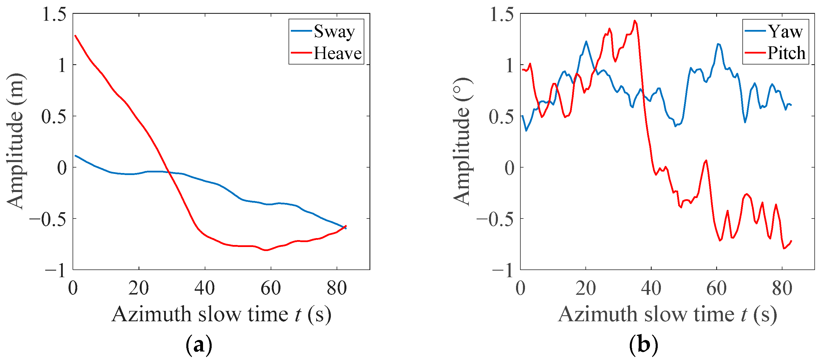
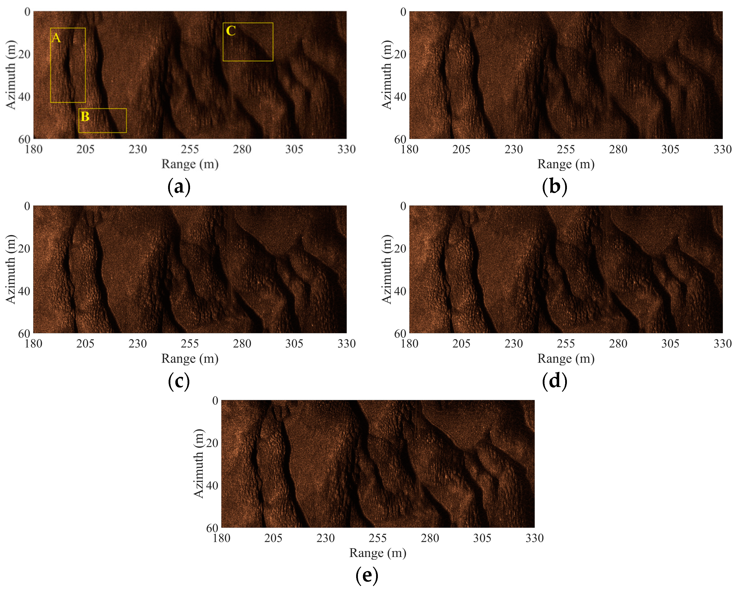
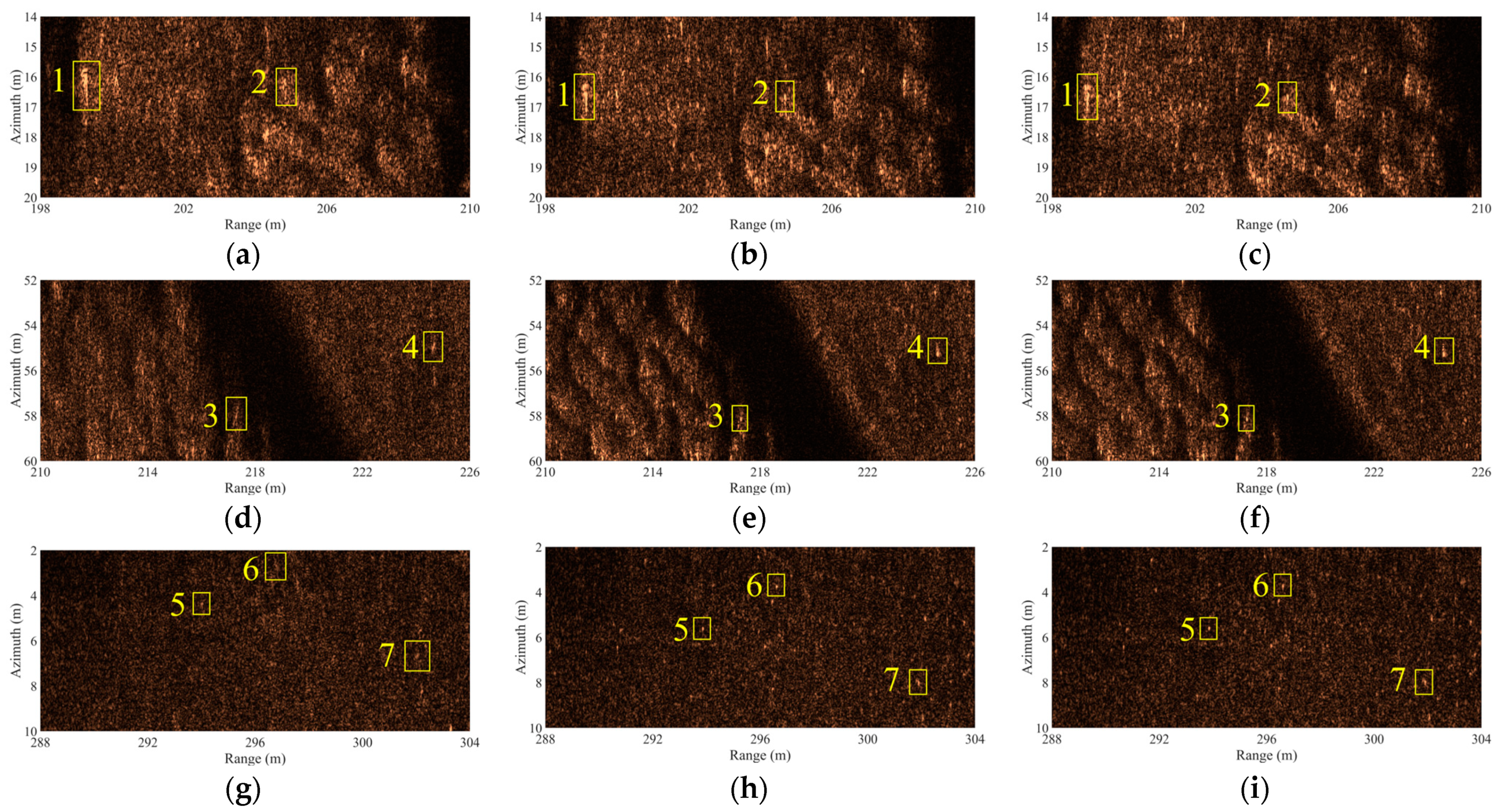
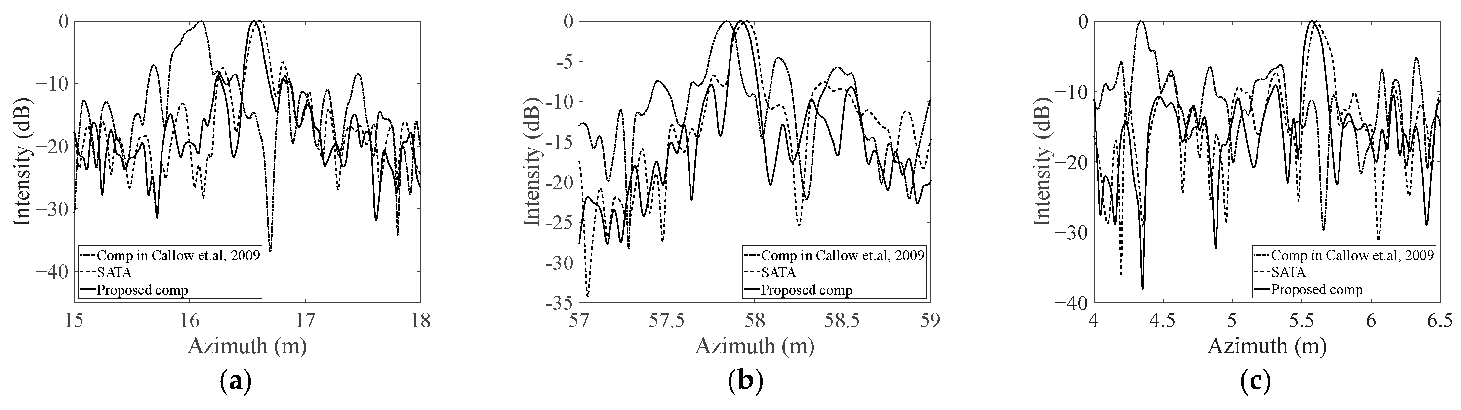
5.3. Real Experimental Data Imaging

The real experiment data are collected using ChinSAS in a sea trial in 2017. The sway, heave, yaw, and pitch obtained by high-precision motion sensors are shown in Figure 14.

The original imaging result without MOCO is shown in Figure 15a. Due to the obvious motion errors of the sonar platform, the image is seriously defocused. The algorithm in [18], the SATA algorithm, and the proposed algorithm are used for compensation, and the results are shown in Figure 15b–d, respectively. As a comparison, we also provide the imaging result of the back-projection (BP) algorithm, as shown in Figure 15e. The three regions A, B, and C in Figure 15a are compared in more detail later.

It can be observed from Figure 15 that the point-like targets are severely defocused in azimuth before compensating, and some terrain contour edges are severely blurred. After the compensation of the above three algorithms, the point-like targets can be better focused, and the problem of edge blurring was significantly improved. By comparison, it is found that the compensation results in Figure 15c,d are close, and the compensation result in Figure 15b is significantly worse than that in Figure 15d. For example, the azimuth ambiguities in areas A, B, and C are still serious, and some point-like targets are not effectively focused. Some areas in A, B, and C are enlarged as shown in Figure 16 to compare the compensation effects of different algorithms more clearly.

Some point-like targets are marked with yellow boxes in Figure 16, as shown by the numerical labels in the figure. It can be seen that the compensation performance of the three algorithms is obvious but different. After compensation by the algorithm in [18], the point-like targets are also wide in azimuth and range directions, and the focusing quality is worse, which is related to the error caused by heave and pitch and the residual 2D spatial-variant RCM. After compensation by the proposed algorithm, the azimuth focus of point-like targets becomes more apparent, which can clearly distinguish point-like targets from the background, making the overall compensation quality better than the algorithm in [18]. From the perspective of visual effects, the compensation effect of the SATA algorithm is also better than the algorithm in [18] and seems to be very close to the proposed algorithm.

To quantitatively compare the compensation results, Figure 17 shows the azimuth profiles of different point-like targets, and

Table 3. Parameters after compensation.

Algorithm	Time (s)	SSIM	Target	IRW (cm)	PSLR (dB)	ISLR (dB)
Compensation in [18]	4.98	0.34	1	27.15	−7.97	−3.83
			3	15.60	−4.53	−0.12
			5	10.61	−4.17	1.17
SATA	2.73	0.49	1	15.87	−6.56	−3.59
			3	15.56	−6.77	−2.19
			5	15.01	−7.26	−2.91
Proposed compensation	4.67	0.57	1	13.55	−8.77	−4.26
			3	12.70	−7.92	−3.37
			5	13.34	−9.13	−4.44

shows the IRW, PSLR, and ISLR values, as well as the calculation time of the three algorithms. In addition, Table 3 also shows the image structure similarity (SSIM) index [42] for the imaging results of the three algorithms and the BP algorithm, which varies from −1 to 1. The closer the value is to 1, the closer the imaging results are to the BP algorithm. The BP algorithm can compensate for arbitrary motion errors and theoretically has the best imaging result. Therefore, the SSIM index is used to quantify the compensation effect of the entire image.

The targets in Figure 17 and Table 3 are marked with yellow boxes in Figure 16. The positions, background strengths, and whether the three targets are located at the edge of the terrain contour are different, so their analyses are representative. As can be seen from Figure 17, the peak positions of the algorithm in [18] have a significant deviation from the SATA algorithm and the algorithm in this paper, and high sidelobes are easily considered false targets. Compared with the SATA algorithm, the sidelobe of the proposed algorithm is lower. The azimuth profiles in Figure 17 indicate that the compensation performance of the proposed algorithm in this paper is superior to the other two algorithms. As can be seen from Table 3, the IRW, PSLR, and ISLR values of the algorithm in this paper are essentially always optimal. Although the IRW value of target 5 after compensation by the algorithm in [18] is better than that of the algorithm in this paper, the corresponding PSLR and ISLR values are far worse than those of the proposed algorithm. A positive ISLR value indicates that the sidelobe energy exceeds the main lobe energy and cannot achieve better-focusing effects. In terms of computing time, the algorithm in this paper is higher than the SATA algorithm and is equivalent to the algorithm in [18], which is consistent with the simulation experiment results. In terms of SSIM, the proposed algorithm is higher than the other two algorithms, indicating that the imaging result of the proposed algorithm is closer to that of the BP algorithm.

In summary, the experimental results of real data are consistent with those of the previous simulated data, which demonstrate the validity of the proposed algorithm in practical applications. Compared with the compensation algorithm in [18] and the SATA algorithm, the compensation performance of the algorithm in this paper is better.

6. Conclusions

In the motion compensation based on motion sensors for wide-beam, multiple-receiver SAS systems, whether the range history error is accurate enough and how to compensate the azimuth-variant range history error are the key to the compensation quality. The existing MOCO algorithms for wide-beam, multiple-receiver SASs are usually based on the stop-hop-stop mode, ignoring the pitch and heave, and do not correct the residual 2D spatial-variant RCM caused by the RSVT. The above factors degrade the MOCO performance. In this paper, we derive the exact expression of the range history error concerning the five-DOF motion errors of the sway, heave, yaw, pitch, and roll under the non-stop-hop-stop case for the first time. Then, we analyze the 2D spatial-variant characteristics of range history error under normal actual motion errors. On this basis, we propose a two-stage subaperture MOCO algorithm for wide-beam, multiple-receiver SAS systems. The algorithm decomposes the range history error into the BCT and the RSVT for compensation, respectively. The first stage of the algorithm compensates for the time delay and phase error caused by the BCT, similar to existing general algorithms. In the second stage, besides the residual phase error compensation in existing algorithms, we additionally correct the residual 2D spatial-variant RCM caused by the RSVT, which has not been considered in the existing subaperture algorithms. The computational complexity of the algorithm only increases moderately.

The simulation results show that the residual phase error of this algorithm after compensation is minimal and meets the imaging requirements of less than one-eighth of the wavelength. Simulated and real-data experiments indicate that the compensation performance of the proposed algorithm is better than existing algorithms and is robust under different distributed motion errors.

Although this algorithm is proposed for wide-beam systems, it is also suitable for narrow-beam systems. The algorithm in this paper can be used as a pre-compensation process before imaging, which is convenient to combine with various imaging algorithms.

References

1. Hansen, R.E.; Callow, H.J.; Sæbø, T.O.; Synnes, S.A.V. Challenges in seafloor imaging and mapping with synthetic aperture sonar. IEEE Trans. Geosci. Remote Sens. 2011, 49, 3677–3687. [Google Scholar] [CrossRef]
2. Zhang, X.; Ying, W. Multireceiver SAS Imagery Based on Monostatic Conversion. IEEE J. Sel. Top. Appl. Earth Obs. Remote Sens. 2021, 14, 10835–10853. [Google Scholar] [CrossRef]
3. Zhang, P.; Tang, J.; Zhong, H.; Ning, M.; Liu, D.; Wu, K. Self-trained target detection of radar and sonar images using automatic deep learning. IEEE Trans. Geosci. Remote Sens. 2022, 60, 4701914. [Google Scholar] [CrossRef]
4. Zhang, X.; Ying, W. Wide-bandwidth Signal-based Multireceiver SAS Imagery Using Extended Chirp Scaling Algorithm. IET Radar Sonar Navig. 2022, 16, 531–541. [Google Scholar] [CrossRef]
5. Raven, R.S. Electronic Stabilization for Displaced Phase Center Systems. U.S. Patent 4,244,036, 6 January 1981. [Google Scholar]
6. Zhang, X.; Zhou, M. Multireceiver SAS Imagery with Generalized PCA. IEEE Geosci. Remote Sens. Lett. 2023, 20, 1502205. [Google Scholar] [CrossRef]
7. Jiang, Z.; Liu, W.; Li, B.; Liu, J.; Zhang, C. A motion compensation method for synthetic aperture sonar based on segment displaced phases center algorithm and errors fitting. J. Electron. Inf. Technol. 2013, 35, 1185–1189. [Google Scholar] [CrossRef]
8. Caporale, S.; Petillot, Y. A novel motion compensation approach for SAS. In Proceedings of the 2016 Sensor Signal Processing for Defence (SSPD), Edinburgh, UK, 22–23 September 2016; pp. 1–5. [Google Scholar]
9. Leier, S.; Zoubir, A.M. Time delay estimation for motion compensation and bathymetry of SAS systems. In Proceedings of the 2012 20th European Signal Processing Conference (EUSIPCO), Bucharest, Romania, 27–31 August 2012; pp. 2293–2297. [Google Scholar]
10. Huxtable, B.D.; Geyer, E.M. Motion compensation feasibility for high resolution synthetic aperture sonar. In Proceedings of the MTS/IEEE OCEANS Conference, Victoria, BC, Canada, 18–21 October 1993; Volume 1, pp. I125–I131. [Google Scholar]
11. Callow, H.J.; Hayes, M.P.; Gough, P.T. Autofocus of stripmap SAS data using the range variant SPGA algorithm. In Proceedings of the MTS/IEEE OCEANS Conference, San Diego, CA, USA, 22–26 September 2003; Volume 5, pp. 2422–2426. [Google Scholar]
12. Hansen, R.E.; Sæbø, T.O.; Gade, K.; Chapman, S. Signal processing for AUV based interferometric synthetic aperture sonar. In Proceedings of the IEEE/MTS OCEANS Conference, San Diego, CA, USA, 22–26 September 2003; Volume 5, pp. 2438–2444. [Google Scholar]
13. Cook, D.A.; Christoff, J.T.; Fernandez, J.E. Motion compensation of AUV-based synthetic aperture sonar. In Proceedings of the MTS/IEEE OCEANS Conference, San Diego, CA, USA, 22–26 September 2003; Volume 4, pp. 2143–2148. [Google Scholar]
14. Ma, M.; Tang, J.; Tian, Z.; Chen, Z. Motion compensation of multiple-receiver synthetic aperture sonar based on high-precision inertial navigation system. J. Huazhong Univ. Sci. Tech. (Nat. Sci. Ed.) 2020, 48, 73–78. [Google Scholar] [CrossRef]
15. Li, H.; Tang, J.; Yuan, B. The integrated navigation underwater used in SAS motion compensation. In Proceedings of the 2009 Second International Conference on Intelligent Computation Technology and Automation, Changsha, China, 11 October 2009. [Google Scholar] [CrossRef]
16. Huang, J.; Tang, J.; Wang, Q.; Wu, W. Motion Compensation in SAS with Multiple Receivers Based on ISCFT Imaging Algorithm. In Proceedings of the 2010 2nd International Conference on Information Engineering and Computer Science, Wuhan, China, 25–26 December 2010. [Google Scholar] [CrossRef]
17. Ma, M.; Tang, J.; Tian, Z.; Zhong, H. Trajectory deviations in narrow-beam SAS: Analysis and compensation. In Proceedings of the 2018 11th International Congress on Image and Signal Processing, BioMedical Engineering and Informatics (CISP-BMEI), Beijing, China, 13–15 October 2018. [Google Scholar]
18. Callow, H.J.; Hayes, M.P.; Gough, P.T. Motion-compensation improvement for widebeam, multiple-receiver SAS systems. IEEE J. Ocean. Eng. 2009, 34, 262–268. [Google Scholar] [CrossRef]
19. Zhu, S.; Hu, J.; Tang, J.; Zhang, S. Simulation of SAS angular motion compensation. J. Syst. Simul. 2009, 21, 6564–6567. [Google Scholar] [CrossRef]
20. Yin, H.; Liu, J.; Zhang, C. Motion compensation of synthetic aperture sonar based on inertial measuring system. J. Electron. Inf. Technol. 2007, 29, 63–66. [Google Scholar]
21. Wu, H.; Tang, J.; Zhong, H.; Tong, Y. An azimuth-variant yaw angle compensation algorithm for multi-aperture synthetic aperture sonar with narrow beam. J. Nav. Univ. Eng. 2019, 31, 37–43. [Google Scholar] [CrossRef]
22. Wilkinson, D.R. Efficient Image Reconstruction Techniques for a Multiple-Receiver Synthetic Aperture Sonar. Master’s Thesis, Department of Electrical and Computer Engineering, University of Canterbury, Christchurch, New Zealand, 2001. [Google Scholar]
23. Moreira, A.; Mittermayer, J.; Scheiber, R. Extended Chirp Scaling Algorithm for Air- and Spaceborne SAR Data Processing in Stripmap and ScanSAR Imaging Modes. IEEE Trans. Geosci. Remote Sens. 1996, 34, 1123–1136. [Google Scholar] [CrossRef]
24. Yang, M.; Zhu, D.; Song, W. Comparison of two-step and one-step motion compensation algorithms for airborne synthetic aperture radar. Electron. Lett. 2015, 51, 1108–1110. [Google Scholar] [CrossRef]
25. Callow, H.J. Signal Processing for Synthetic Aperture Sonar Image Enhancement. Ph.D. Thesis, Dept. Electr. Electron. Eng., Univ. Canterbury, Christchurch, New Zealand, 2003. [Google Scholar]
26. Sæbø, T.O.; Langli, B.; Callow, H.J.; Hammerstad, E.O.; Hansen, R.E. Bathymetric capabilities of the HISAS interferometric synthetic aperture sonar. In Proceedings of the MTS/IEEE OCEANS Conference, Vancouver, BC, Canada, 29 September–4 October 2007; pp. 1–10. [Google Scholar]
27. Châtillon, J.; Adams, A.E.; Lawlor, M.A.; Zakharia, M.E. SAMI: A low-frequency prototype for mapping and imaging of the seabed by means of synthetic aperture. IEEE J. Ocean. Eng. 1999, 24, 4–15. [Google Scholar] [CrossRef]
28. Warman, K.; Chick, K.; Chang, E. Synthetic aperture sonar processing for widebeam/broadband data. In Proceedings of the MTS/IEEE OCEANS Conference, Honolulu, HI, USA, 5–8 November 2001; Volume 1, pp. 208–211. [Google Scholar]
29. Hayes, M.P.; Gough, P.T. Synthetic aperture sonar: A review of current status. IEEE J. Ocean. Eng. 2009, 34, 207–224. [Google Scholar] [CrossRef]
30. Potsis, A.; Reigber, A.; Mittermayer, J.; Moreira, A.; Uzunoglou, N. Sub-aperture algorithm for motion compensation improvement in wide-beam SAR data processing. Electron. Lett. 2001, 37, 1405–1407. [Google Scholar] [CrossRef]
31. Prats, P.; Reigber, A.; Mallorqui, J.J. Topography-dependent motion compensation for repeat-pass interferometric SAR systems. IEEE Geosci. Remote Sens. Lett. 2005, 2, 206–210. [Google Scholar] [CrossRef]
32. Scheiber, R.; Bothale, V.M. Interferometric multi-look techniques for SAR data. In Proceedings of the IEEE IGARSS, Toronto, ON, Canada, 24–28 June 2002; Volume 1, pp. 173–175. [Google Scholar]
33. Zheng, X.; Yu, W.; Li, Z. A novel algorithm for wide beam SAR motion compensation based on frequency division. In Proceedings of the IGARSS, Denver, CO, USA, 31 July–4 August 2006; pp. 3160–3163. [Google Scholar]
34. de Macedo, K.A.C.; Scheiber, R. Precise topography- and aperture-dependent motion compensation for airborne SAR. IEEE Geosci. Remote Sens. Lett. 2005, 2, 172–176. [Google Scholar] [CrossRef]
35. Prats, P.; de Macedo, K.A.C.; Reigber, A.; Scheiber, R.; Scheiber, R. Comparison of topography- and aperture-dependent motion compensation algorithms for airborne SAR. IEEE Geosci. Remote Sens. Lett. 2007, 4, 349–353. [Google Scholar] [CrossRef]
36. Zhang, X.; Tang, J.; Zhong, H.; Zhang, S. Wavenumber-domain imaging algorithm for wide-beam multi-receiver synthetic aperture sonar. J. Harbin Eng. Univ. 2014, 35, 93–101. [Google Scholar]
37. Bamler, R. A comparison of range-Doppler and wavenumber domain SAR focusing algorithms. IEEE Trans. Geosci. Remote Sens. 1992, 30, 706–713. [Google Scholar] [CrossRef]
38. Kirk, J.C. Motion compensation for synthetic aperture radar. IEEE Trans. Aerosp. Electron. Syst. 1975, AES-11, 338–348. [Google Scholar] [CrossRef]
39. Xue, G. Research of Motion Compensation in Airborne UWB SAR with High Resolution. Ph.D. Thesis, National University of Defense Technology, Changsha, China, 2008. [Google Scholar]
40. Xu, J.; Tang, J.; Zhang, C.; Zhou, S.; Zhou, L. Multi-aperture synthetic aperture sonar imaging algorithm. Signal Process. 2003, 19, 157–160. [Google Scholar] [CrossRef]
41. Hagen, P.E.; Hansen, R.E. Post-mission analysis with the HUGIN AUV and high-resolution interferometric SAS. In Proceedings of the MTS/IEEE OCEANS Conference, Boston, MA, USA, 18–22 September 2006; pp. 1–6. [Google Scholar]
42. Wang, Z.; Bovik, A.C. A universal image quality index. IEEE Signal Process. Lett. 2002, 9, 81–84. [Google Scholar] [CrossRef]
Figure 1. Motion geometry of multiple-receiver SAS.
Jmse 11 01627 g001
Figure 2. SAS attitude diagram. The center of the transmitter is located at the origin, and d i denotes the distance between the center of the receiver i and the center of the transmitter. ψ , θ , and φ are yaw, pitch, and roll, respectively.
Jmse 11 01627 g002
Figure 3. Actual motion errors of real experimental data: (a) translational motion errors; (b) rotational motion errors.
Jmse 11 01627 g003
Figure 4. Schematic diagram of SAS collecting data.
Jmse 11 01627 g004
Figure 5. Curve of the BCT and RSVT with receivers: (a) BCT; (b) RSVT at the range of 100 m.
Jmse 11 01627 g005
Figure 6. Range spatial-variant characteristics of BCT: (a) severe motion errors; (b) slight motion errors.
Jmse 11 01627 g006
Figure 7. Spatial-variant characteristics of RSVT: (a) variation with range and azimuth; (b) variation of beam edge with range.
Jmse 11 01627 g007
Figure 8. Block diagram of the subaperture MOCO algorithm for multiple-receiver SAS systems.
Jmse 11 01627 g008
Figure 9. Residual phase error after compensation: (a) SATA algorithm; (b) proposed algorithm.
Jmse 11 01627 g009
Figure 10. Imaging swath and motion errors: (a) schematic diagram of the targets in the swath; (b) sinusoidal motion errors; (c) cubic polynomial motion errors; (d) uniform random motion errors.
Jmse 11 01627 g010aJmse 11 01627 g010b
Figure 11. Comparison of imaging results using the three compensation algorithms under different distributed motion errors: (ac) sinusoidal motion errors, (df) cubic polynomial motion errors, and (gi) uniform random motion errors. (a,d,g) are the compensation results of the algorithm in [18]. (b,e,h) are the compensation results of the SATA algorithm. (c,f,i) are the compensation results of the proposed algorithm.
Jmse 11 01627 g011
Figure 12. Compensation results of target 1 under different distributed motion errors using the three algorithms: (a) the result of the algorithm in [18] under sinusoidal motion errors; (b) the result of the SATA algorithm under sinusoidal motion errors; (c) the result of the proposed algorithm under sinusoidal motion errors; (d) the result of the algorithm in [18] under cubic polynomial motion errors; (e) the result of the SATA algorithm under cubic polynomial motion errors; (f) the result of the proposed algorithm under cubic polynomial motion errors; (g) the result of the algorithm in [18] under uniform random motion errors; (h) the result of the SATA algorithm under uniform random motion errors; (i) the result of the proposed algorithm under uniform random motion errors.
Jmse 11 01627 g012
Figure 13. Comparison of the azimuth profiles of target 1 using the three compensation algorithms: (a) sinusoidal motion errors; (b) cubic polynomial motion errors; (c) uniform random motion errors [18].
Jmse 11 01627 g013
Figure 14. Actual motion errors of real experimental data.
Jmse 11 01627 g014
Figure 15. Imaging results of the compensation algorithms: (a) no compensation; (b) wide-beam compensation in [18]; (c) SATA algorithm; (d) compensation proposed in this paper; (e) BP algorithm.
Jmse 11 01627 g015
Figure 16. Imaging results of different regions using the three compensation algorithms. (a,d,g) are the results of compensation in [18]. (b,e,h) are the results of the SATA algorithm. (c,f,i) are the results of the proposed compensation algorithm.
Jmse 11 01627 g016
Figure 17. Comparison of the azimuth profiles for different targets using the three compensation algorithms: (a) target 1; (b) target 3; (c) target 5 [18].
Jmse 11 01627 g017