
Numerical and Experimental Investigations on Non-Linear Wave Action on Offshore Wind Turbine Monopile Foundation


Abstract
:1. Introduction
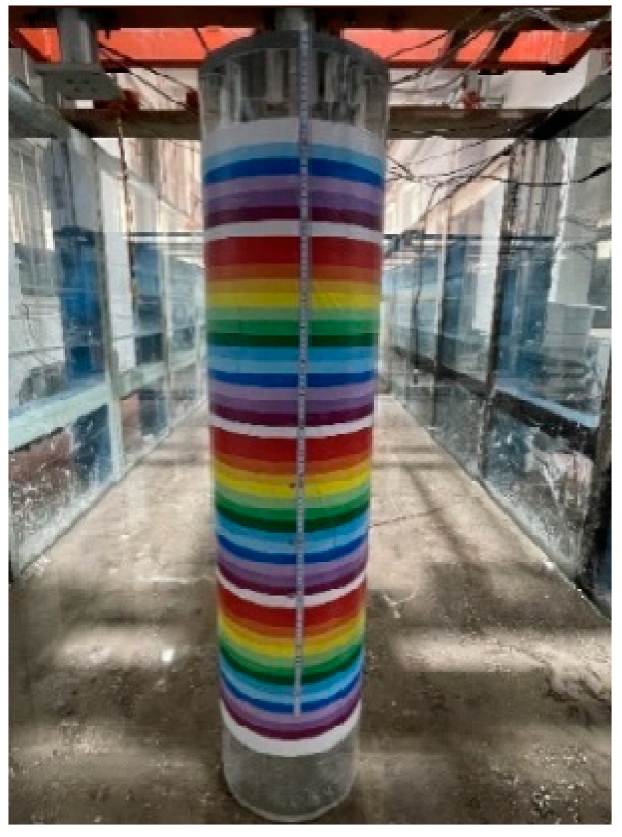
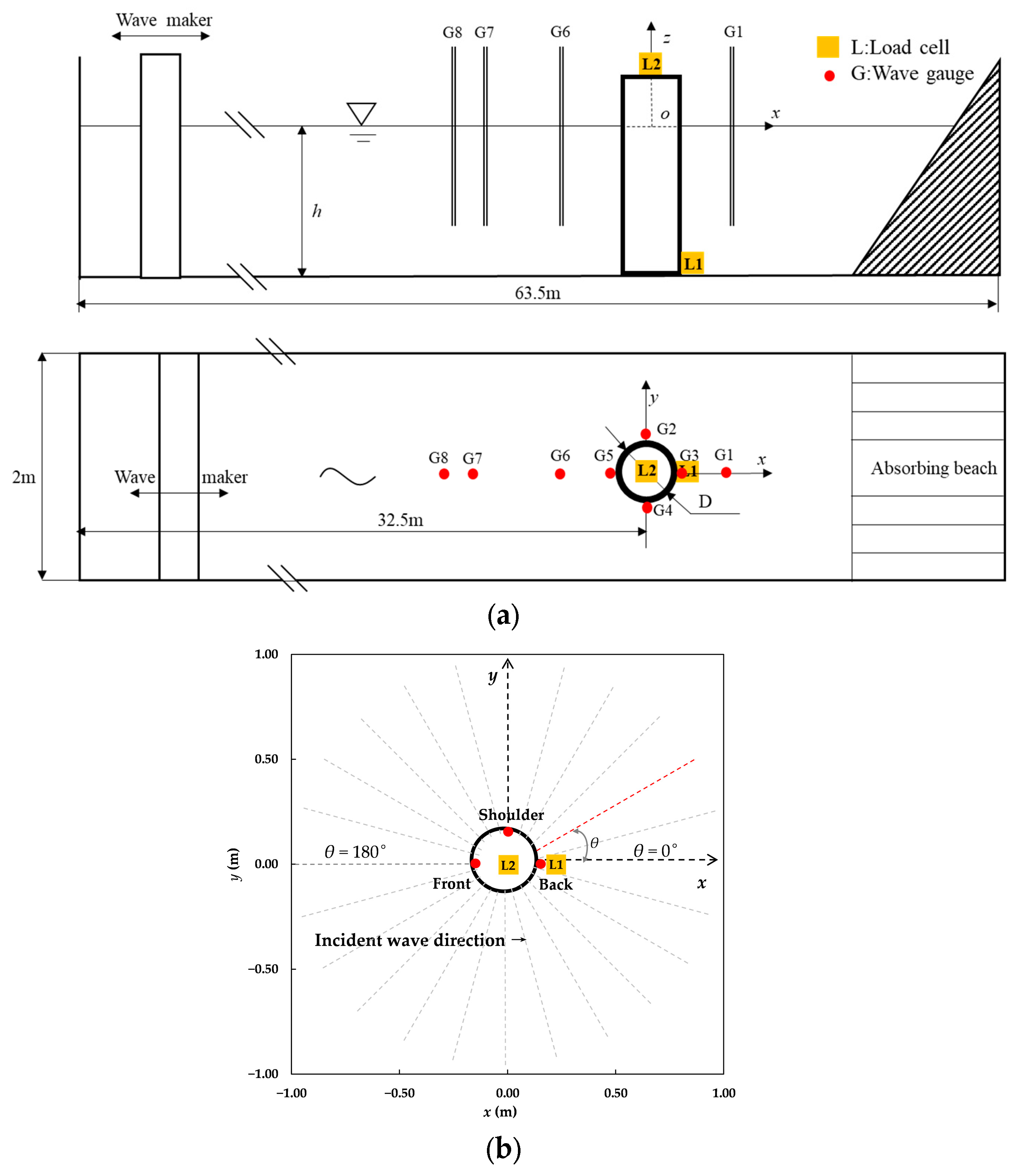
2. Experiments
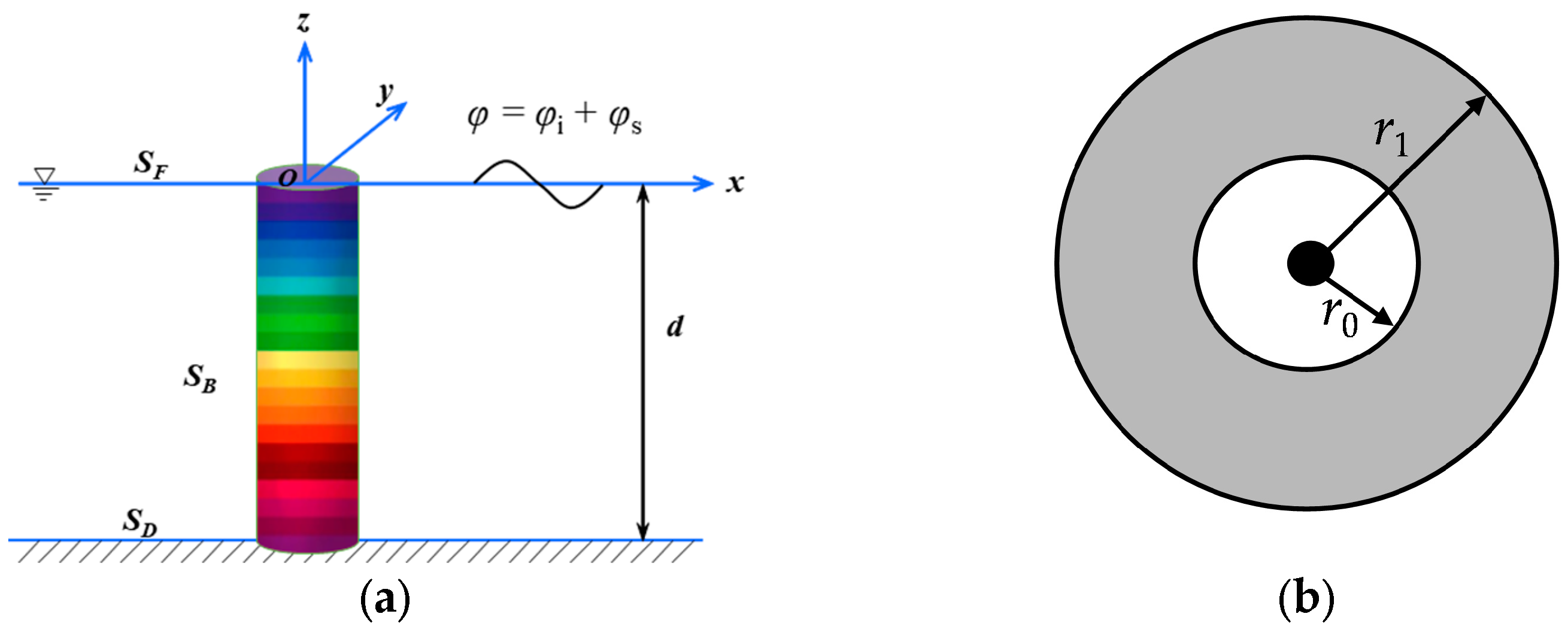
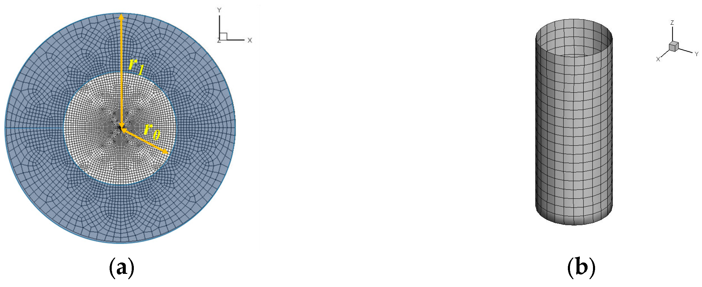
3. Numerical Methodology
4. Results and Discussion
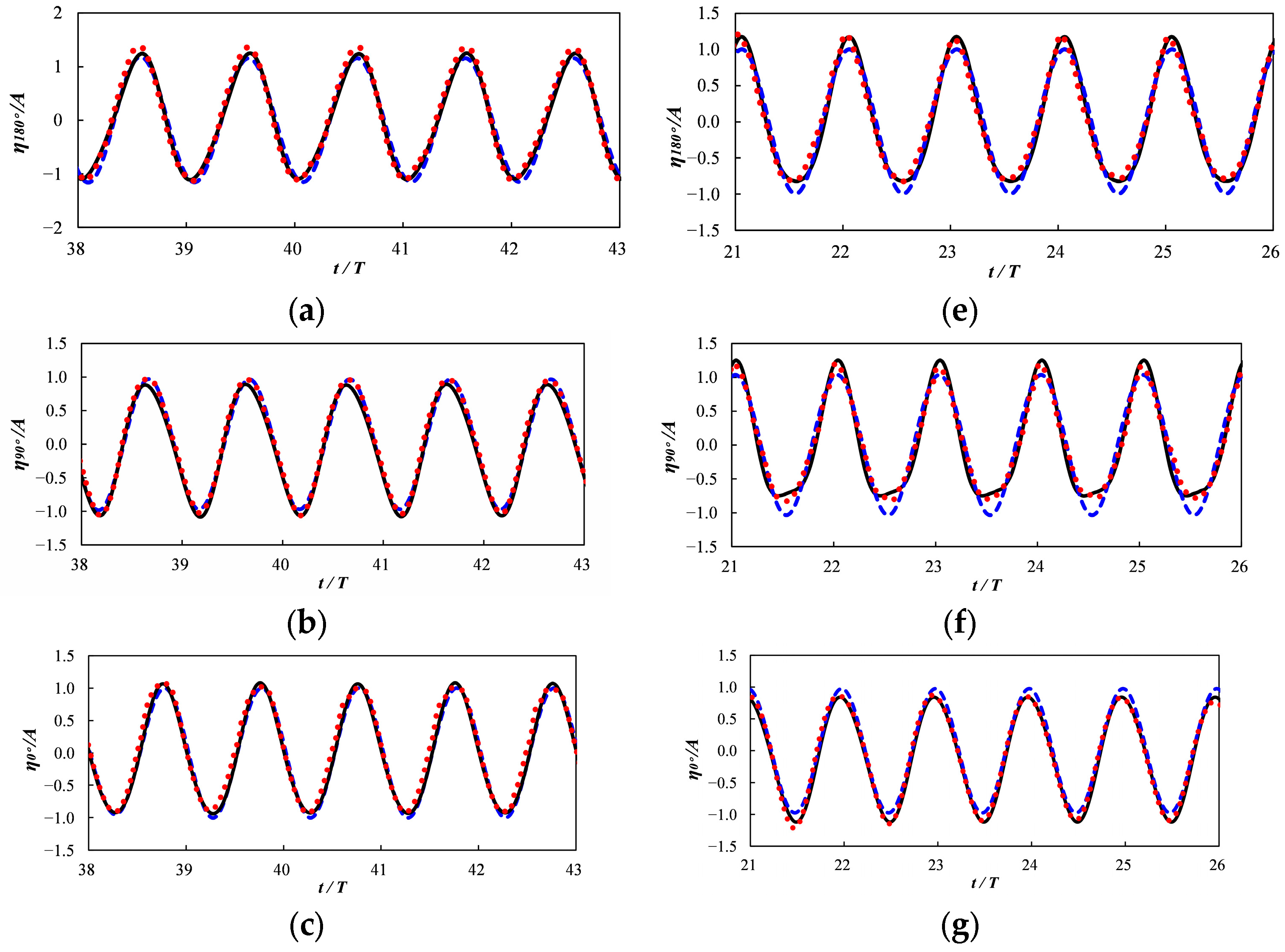
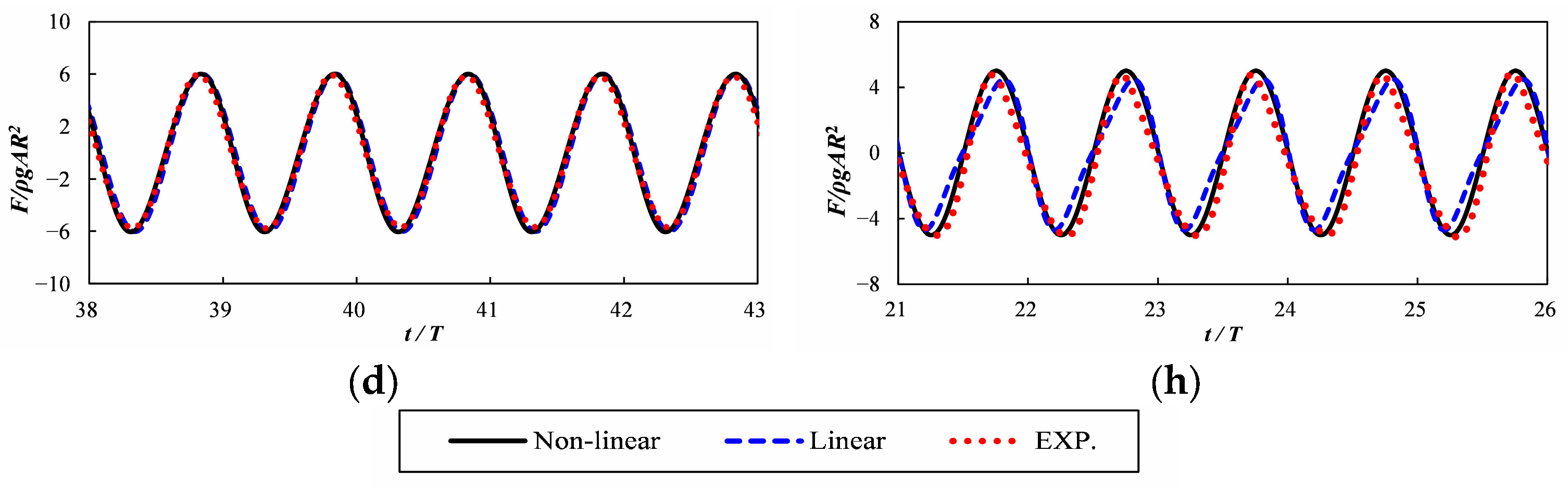
4.1. Comparisons between the Numerical and Experimental Results
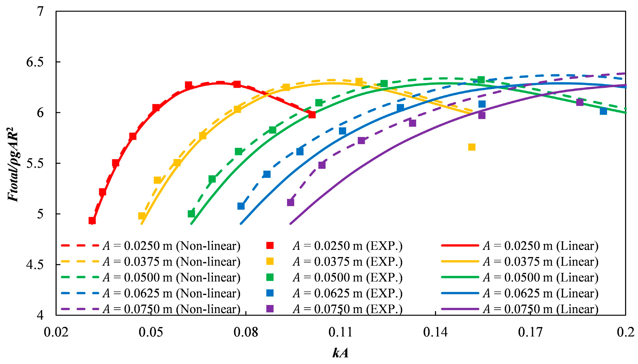
4.2. Wave Load on the Monopile
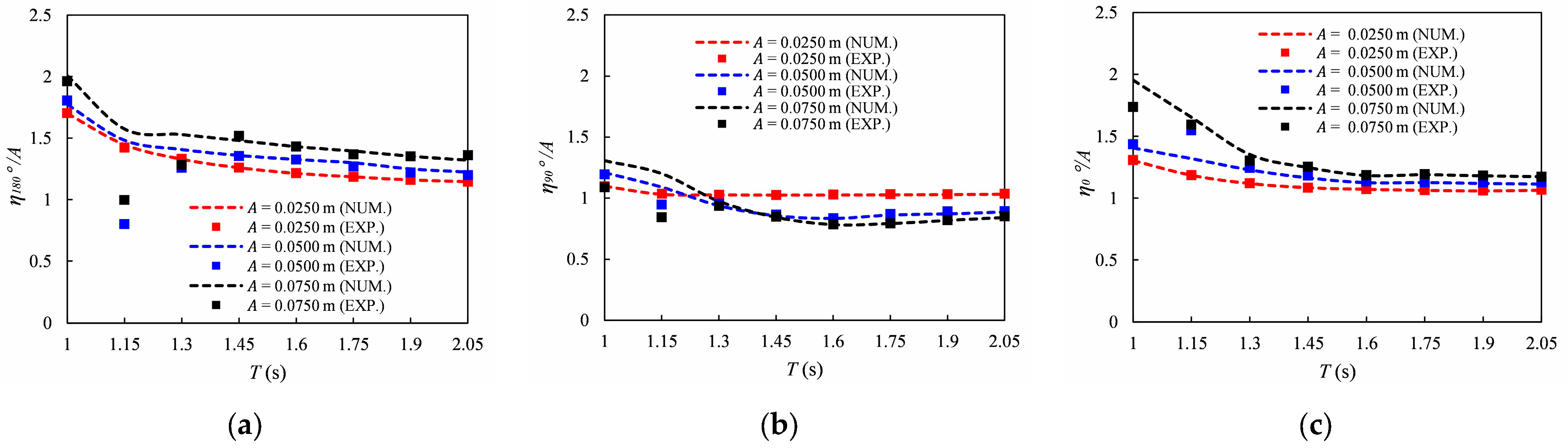
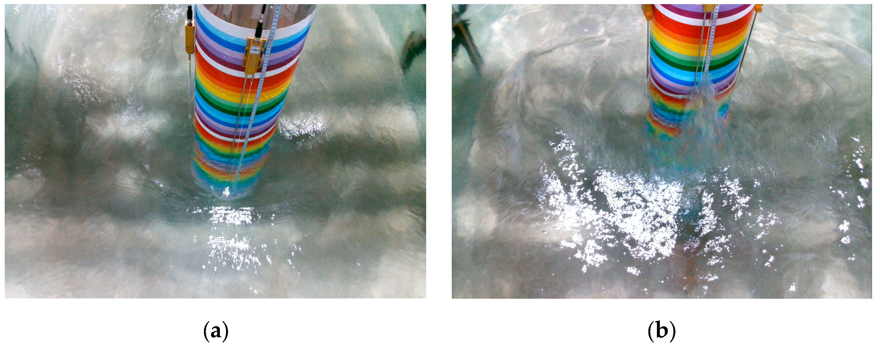
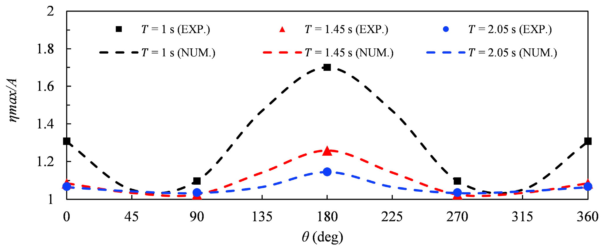
4.3. Run-Up on the Monopile
5. Harmonic Structure on Monopile
5.1. Harmonic Wave Load Component
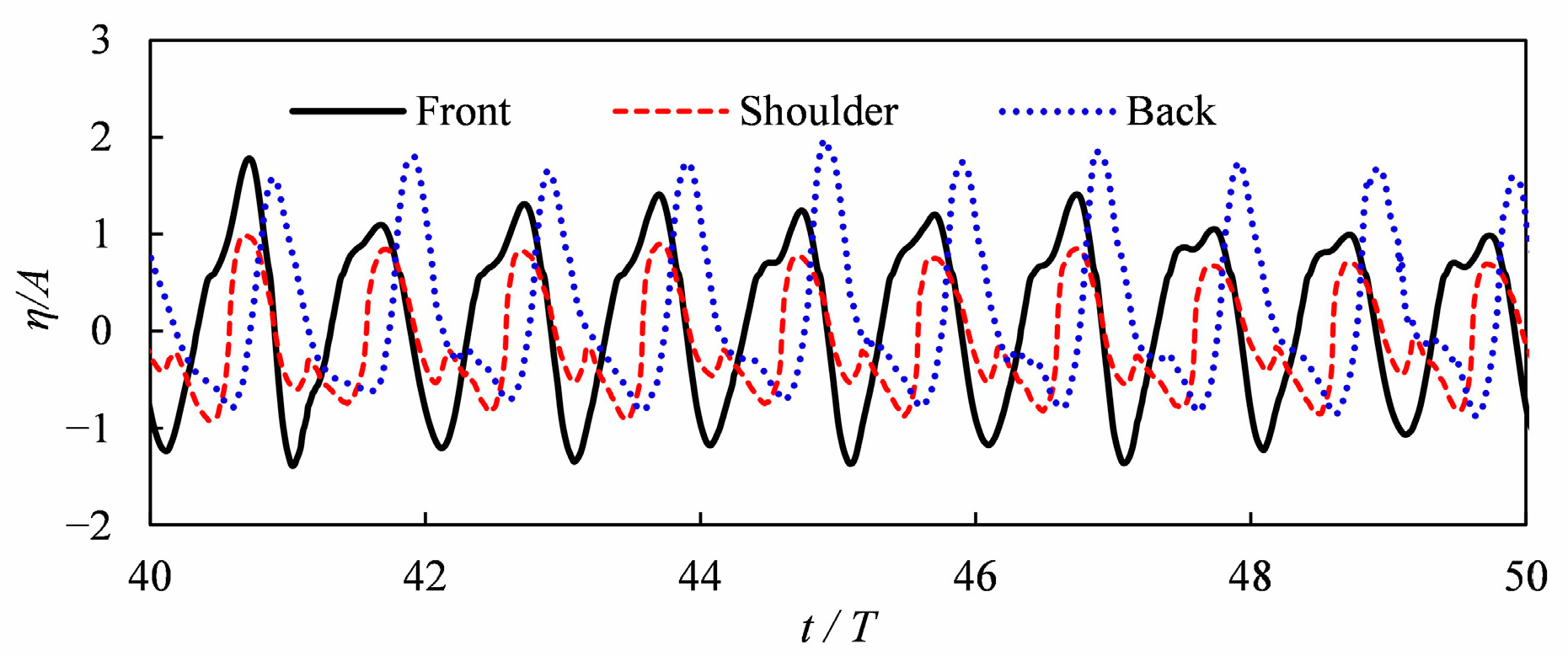
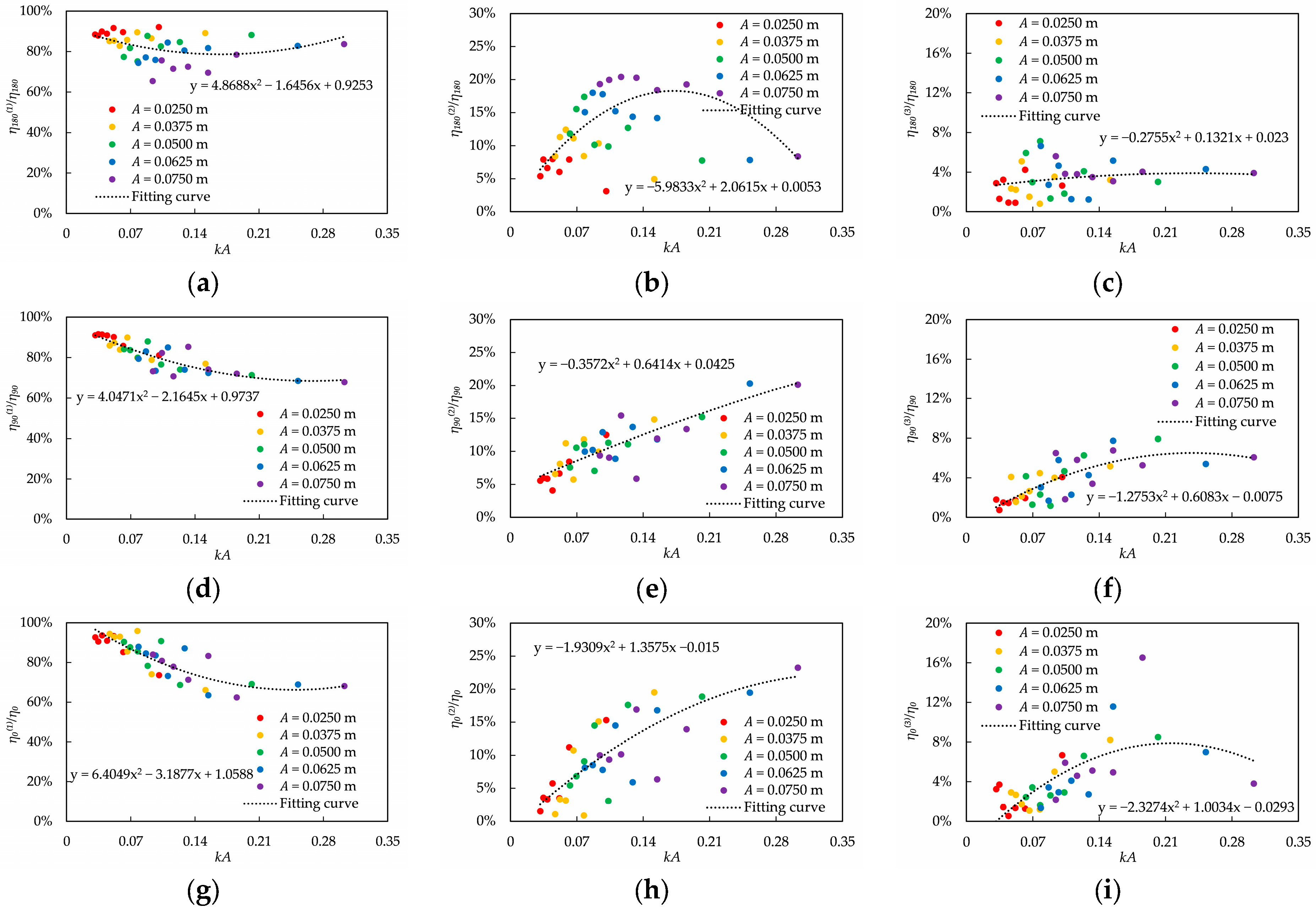
5.2. Harmonics of Wave Run-Up Component
6. Concluding Remarks and Future Works
6.1. Concluding Remarks
6.2. Future Works
Author Contributions
Funding
Institutional Review Board Statement
Informed Consent Statement
Data Availability Statement
Conflicts of Interest
References
- International Energy Agency. Offshore Wind Outlook 2021. World Energy Outlook Special Report; International Energy Agency: Paris, France, 2022. [Google Scholar]
- Butterfield, S.; Musial, W.; Jonkman, J.; Sclavounos, P. Engineering Challenges for Floating Offshore Wind Turbines. In Proceedings of the 2005 Copenhagen Offshore Wind Conference, Copenhagen, Denmark, 26–28 October 2005. [Google Scholar]
- Gao, Z.; Bingham, H.; Nicolls-Lee, R.; Adam, F.; Ren, H. Proceedings of the Offshore Renewable Energy, 19th ISSC Congress, Cascais, Portugal, 7–10 September 2015.
- Corvaro, S.; Marini, F.; Mancinelli, A.; Lorenzoni, C.; Brocchini, M. Hydro- and Morpho-dynamics Induced by a Vertical Slender Pile under Regular and Random Waves. J. Waterw. Port Coast. Ocean. Eng. 2018, 144, 04018018. [Google Scholar] [CrossRef]
- Corvaro, S.; Crivellini, A.; Marini, F.; Cimarelli, A.; Capitanelli, L.; Mancinelli, A. Experimental and numerical analysis of the hydrodynamics around a vertical cylinder in waves. J. Mar. Sci. Eng. 2019, 7, 453. [Google Scholar] [CrossRef]
- Sumer, B.M.; Fredse, J. The mechanics of scour in the marine environment. In Advanced Series on Ocean Engineering; World Scientific: Singapore, 2002; Volume 17. [Google Scholar]
- Abhinav, K.; Saha, N. Dynamic analysis of monopile supported offshore wind turbines. Geotech. Eng. 2017, 170, 428–444. [Google Scholar] [CrossRef]
- Ma, H.; Yang, J. A novel hybrid monopile foundation for offshore wind turbines. Ocean. Eng. 2020, 198, 106963. [Google Scholar] [CrossRef]
- Zhou, Y.; Ning, D.; Shi, W. Hydrodynamic investigation on an OWC wave energy converter integrated into an OWT monopile. Coast. Eng. 2020, 162, 103731. [Google Scholar] [CrossRef]
- Zeng, X.; Shi, W.; Michailides, C.; Zhang, S.; Li, X. Numerical and experimental investigation of breaking wave forces on a monopile-type offshore wind turbine. Renew. Energy 2021, 175, 501–519. [Google Scholar] [CrossRef]
- Grue, J.; Bjorshol, G.; Strand, O. Nonlinear wave loads which may generate ‘ringing’ responses of offshore structures. In Proceedings of the International Workshop on Water Waves and Floating Bodies, Osaka, Japan, 17–20 April 1994. [Google Scholar]
- Chaplin, J.R.; Rainey, R.C.T.; Yemm, R.W. Ringing of a vertical cylinder in waves. J. Fluid Mech. 1900, 350, 119–147. [Google Scholar] [CrossRef]
- Huseby, M.; Grue, J. An experimental investigation of higher-harmonic wave forces on a vertical cylinder. J. Fluid Mech. 2000, 414, 75–103. [Google Scholar] [CrossRef]
- Lee, C. WAMIT Theory Manual; Massachusetts Institute of Technology, Department of Ocean Engineering: Cambridge, MA, USA, 1995. [Google Scholar]
- DNV, G.L. SESAM User Manual; WADAM: Høvik, Norway, 2019. [Google Scholar]
- ANSYS. AQWA Theory Manual; ANSYS: Canonsburg, PA, USA, 2013. [Google Scholar]
- Jonkman, J.M.; Buhl, M.L. FAST User’s Guide; National Renewable Energy: Salt Lake City, UT, USA, 2005. [Google Scholar]
- MacCamy, R.C.; Fuchs, R.A. Wave forces on piles: A diffraction theory. Beach Erosion board office of the chief engineers, department of the army. Tech. Memo. 1954, 69, 1–17. [Google Scholar]
- Morris-Thomas, M.T.; Thiagarajan, K.P. The run up on a cylinder in progressive surface gravity waves: Harmonic components. Appl. Ocean. Res. 2004, 26, 98–113. [Google Scholar] [CrossRef]
- Niedzwecki, J.M.; Duggal, A.S. Wave run-up and forces on cylinders in regular and random waves. J. Waterw. Port Coast. Ocean. Eng. 1992, 118, 615–634. [Google Scholar] [CrossRef]
- Malenica, S.; Molin, B. Third-harmonic wave diffraction by a vertical cylinder. J. Fluid Mech. 1995, 302, 203–229. [Google Scholar] [CrossRef]
- Tromans, P.; Swan, C.; Masterton, S. Nonlinear Potential Flow Forcing: The Ringing of Concrete Gravity-Based Structures; Health and Safety Executive: Bootle, UK, 2006; pp. 4–68. [Google Scholar]
- Chen, L.; Zang, J.; Taylor, P.H.; Sun, L.; Morgan, G.; Grice, J.; Orszaghova, J.; Ruiz, M.T. An experimental decomposition of nonlinear forces on a surface-piercing column: Stokes-type expansions of the force harmonics. J. Fluid. Mech. 2018, 848, 42–77. [Google Scholar] [CrossRef]
- Kristiansen, T.; Faltinsen, O.M. Higher harmonic wave loads on a vertical cylinder in finite water depth. J. Fluid. Mech. 2017, 833, 773–805. [Google Scholar] [CrossRef]
- Stansberg, C.T.; Nielsen, F.G. Nonlinear wave—Structure interaction on floating production systems. In Proceedings of the 11th ISOPE Conference IV, Stavanger, Norway, 17–22 June 2001. [Google Scholar]
- Swan, C.; Masterton, S.; Sheikh, R.; Cavalletti, A. Wave forcing and wave scattering from a vertical surface-piercing cylinder. In Proceedings of the 24th OMAE Conference, Halkidiki, Greece, 12–17 June 2005. [Google Scholar]
- Stansberg, C.T.; Kristiansen, T. Non-linear scattering of steep surface waves around vertical columns. Appl. Ocean Res. 2005, 27, 65–80. [Google Scholar] [CrossRef]
- De Vos, L.; Frigaard, P.; De Rouck, J. Wave run-up on cylindrical and cone shaped foundations for offshore wind turbines. Coast. Eng. 2007, 54, 17–29. [Google Scholar] [CrossRef]
- Kriebel, D. Non-linear wave interaction with a vertical circular cylinder. Part ll: Wave run-up. Ocean Eng. 1992, 19, 75–79. [Google Scholar] [CrossRef]
- Kriebel, D. Technical note nonlinear wave interaction with a vertical circular Cylinder: Wave forces. Ocean. Eng. 1998, 25, 597–605. [Google Scholar]
- Lykke Andersen, T.; Frigaard, P.; Damsgaard, M.L.; De Vos, L. Wave run-up on slender piles in design conditions Model tests and design rules for offshore wind. Coast. Eng. 2011, 58, 281–289. [Google Scholar] [CrossRef]
- Morison, J.; Johnson, J.; Schaaf, S. The force exerted by surface waves on piles. J. Pet Technol. 1950, 2, 149–154. [Google Scholar] [CrossRef]
- Ning, D.Z.; Zang, J.; Liu, S.X.; Taylor, R.E.; Teng, B.; Taylor, P.H. Free-surface evolution and wave kinematics for nonlinear uni-directional focused wave groups. Ocean. Eng. 2009, 36, 1226–1243. [Google Scholar] [CrossRef]
- Soares, C.G. Offshore Structure Modeling; World Scientific: Cambridge, MA, USA, 1995. [Google Scholar]
- Fenton, J.D. Nonlinear Wave Theories, the Sea; Wiley: Hoboken, NJ, USA, 1990; Volume 9. [Google Scholar]
- Taylor, R.E.; Hung, S. Second order diffraction forces on a vertical cylinder in regular waves. Appl. Ocean Res. 1987, 9, 19–30. [Google Scholar] [CrossRef]
- Jin, R.; Teng, B.; Ning, D.Z.; Zhao, M.; Cheng, L. Numerical investigation of influence of wave directionality on the water resonance at a narrow gap between two rectangular barges. Act. Oceanolo. Sin. 2017, 36, 104–111. [Google Scholar] [CrossRef]
- Zhou, B.Z.; Ning, D.Z.; Teng, B.; Bai, W. Numerical investigation of wave radiation by a vertical cylinder using a fully nonlinear HOBEM. Ocean. Eng. 2013, 70, 1–13. [Google Scholar] [CrossRef]


| Position (m) | ||||||||
|---|---|---|---|---|---|---|---|---|
| G1 | G2 | G3 | G4 | G5 | G6 | G7 | G8 | |
| x | 1.5 | 0 | −0.15 | 0 | 0.15 | −1.65 | −4.15 | −4.65 |
| y | 0 | 0.15 | 0 | −0.15 | 0 | 0 | 0 | 0 |
| T (s) kA A (m) | 1.00 | 1.15 | 1.30 | 1.45 | 1.60 | 1.75 | 1.90 | 2.05 |
| 0.0250 | 0.101 | 0.077 | 0.062 | 0.052 | 0.044 | 0.039 | 0.035 | 0.031 |
| 0.0375 | 0.151 | 0.116 | 0.093 | 0.077 | 0.066 | 0.058 | 0.052 | 0.047 |
| 0.0500 | 0.202 | 0.154 | 0.124 | 0.103 | 0.088 | 0.078 | 0.069 | 0.063 |
| 0.0625 | 0.252 | 0.193 | 0.155 | 0.129 | 0.111 | 0.097 | 0.087 | 0.078 |
| 0.0750 | 0.303 | 0.232 | 0.186 | 0.155 | 0.133 | 0.117 | 0.104 | 0.094 |
Disclaimer/Publisher’s Note: The statements, opinions and data contained in all publications are solely those of the individual author(s) and contributor(s) and not of MDPI and/or the editor(s). MDPI and/or the editor(s) disclaim responsibility for any injury to people or property resulting from any ideas, methods, instructions or products referred to in the content. |
© 2023 by the authors. Licensee MDPI, Basel, Switzerland. This article is an open access article distributed under the terms and conditions of the Creative Commons Attribution (CC BY) license (https://creativecommons.org/licenses/by/4.0/).
Share and Cite
Deng, S.; Qin, M.; Ning, D.; Lin, L.; Wu, S.; Zhang, C. Numerical and Experimental Investigations on Non-Linear Wave Action on Offshore Wind Turbine Monopile Foundation. J. Mar. Sci. Eng. 2023, 11, 883. https://doi.org/10.3390/jmse11040883
Deng S, Qin M, Ning D, Lin L, Wu S, Zhang C. Numerical and Experimental Investigations on Non-Linear Wave Action on Offshore Wind Turbine Monopile Foundation. Journal of Marine Science and Engineering. 2023; 11(4):883. https://doi.org/10.3390/jmse11040883
Chicago/Turabian StyleDeng, Sijia, Ming Qin, Dezhi Ning, Lin Lin, Songxiong Wu, and Chongwei Zhang. 2023. "Numerical and Experimental Investigations on Non-Linear Wave Action on Offshore Wind Turbine Monopile Foundation" Journal of Marine Science and Engineering 11, no. 4: 883. https://doi.org/10.3390/jmse11040883