Article

Modeling Impact Load on a Vertical Cylinder in Dam-Break Flows

1
State Key Laboratory of Coastal and Offshore Engineering, Dalian University of Technology, Dalian 116024, China
2
Dalian Key Laboratory of Offshore Renewable Energy, Dalian 116024, China
3
Oceans Graduate School, Faculty of Engineering and Mathematical Sciences, The University of Western Australia, Crawley, WA 6009, Australia
*
Authors to whom correspondence should be addressed.
J. Mar. Sci. Eng. 2023, 11(5), 932; https://doi.org/10.3390/jmse11050932
Submission received: 31 March 2023 / Revised: 21 April 2023 / Accepted: 24 April 2023 / Published: 27 April 2023

Abstract

:
A three-dimensional dam-break flow interacting with a vertical circular and square cylinder is studied in this paper using computational fluid dynamics simulations based on OpenFOAM. This resembles closely a tsunami wave and greenwater flow acting on coastal or on-deck structures, which are of relevance and importance to coastal protections and offshore operations, respectively. The numerical model is verified by comparing with published experimental measurements and is extended to investigate the effects of the structural geometry and the impacting angle β (i.e., the angle between the water front and cylinders) on the total impact load and the surrounding flow field. It is found that the impact event experiences two distinct stages characterized by a constant flow velocity and a negative flow acceleration, respectively. In addition, the total force on a square cylinder is nearly twice that of a circular cylinder although the impacting area is the same. The longitudinal and transverse forces are found to decrease and increase with the impacting angle, respectively. A close interrogation of the surrounding flow field via flow visualization suggests that the way the flow deflected from the cylinder surfaces plays an important role in determining the pressure field and thus the total force behaviors.

1. Introduction

Dam-break flow, incurred by a sudden removal/collapse of a vertical dam/barrier that blocks a mass of water, is of importance in civil engineering. Accurate modeling/prediction of this is challenging yet essential for designing a dam [1]. Recently, the dam-break flow and dam-break models (used for describing dam-break flow evolution, etc.) have also attracted increasing attention in the field of coastal and offshore engineering because these are considered able to accurately describe the behaviors of nearshore tsunami bore [2] and greenwater flow onto a vessel deck [3] to a certain level. A rapidly moving tsunami wave front (e.g., up to 7 m/s for the 2011 Great East Japan Tsunami) poses threats on coastal infrastructures (e.g., buildings and bridges) and even worse, causes losses of life [4]. Greenwater, characterized by a large amount of water being elevated and overtopped onto a vessel deck in extreme seas, is one of the most important issues for, e.g., floating production, storage, and offloading (FPSO) survivability designs [5].
Many theoretical dam-break solutions have been derived by solving shallow water equations without [6] or with hydraulic resistance [7] being represented in the form of basal friction. General good agreements with the experimental measurements in terms of the water profile and the water front velocity (i.e., the velocity of the water front) are achieved [3,8,9,10]. Nevertheless, these models fail to capture forces on structures by the impact of dam-break flows.
Instead, zero-gravity similarity solutions by Cumberbatch [11] derived for a water wave striking on a wall can be applied for estimating the impact force. Here, the shape of the wave before the impact was assumed to be a two-dimensional (2-D) infinite wedge and the effect of gravity was neglected. Cross [12] extended this theory by dividing the total impact force into hydrodynamic and hydrostatic forces. The former was calculated by solutions in Cumberbatch [11]. Kihara [13] claimed that these solutions were not satisfactory, and an overestimation of (30–50) % was observed when compared to the experiments. The law of conservation in momentum flux is also widely applied. For example, Raju [14] estimated the drag force on a circular cylinder in subcritical free surface flows. One of their major assumptions was that the change in the water depths was small upstream and downstream the cylinder. Obviously, this assumption, and thus the methodology, can be inaccurate when applied for modeling forces on three-dimensional (3-D) bodies, where the flow field is extremely unsteady and localized during the impact event [15].
Carefully instrumented physical experiments are then extremely useful for investigating the dam-break flow evolution [16,17] and 3D dam-break–flow–structure interactions [18,19,20]. Quantitative data, including the instantaneous free surface elevations, the pressure on the structure, and the surrounding flow field, were collected and used for validating numerical models. Uncertainties associated with the control over the gate motion [21], and the measuring technique for capturing the pressure and the water front motion, were noted [22]. The widely used PIV (particle image velocimetry) technique for measuring the velocity field within the flow was found to work less well because the flow field was highly three-dimensional and violent splashing occurred during the impact event. It is worth noting that vertical walls and cylinders were considered in these experimental studies.
Recently, advanced 2D and/or 3D CFD-based models were developed [23,24], complementing and extending the experimental studies. In these models, RANS (Reynolds-averaged Navier–Stokes) equations coupled with a turbulence closure model were used to describe the behaviors of turbulent dam-break flows. For example, Park [25,26] used Fluent, a commercial CFD software, to investigate the influence of the initial turbulence intensity (TI) on the evolution of a dam-break flow. TI represents the intensity of velocity fluctuation, hence its initial value cannot be calculated theoretically (as for initial still water, the velocity fluctuation is zero). Its initial value is usually determined empirically and then is iteratively corrected by comparing the experimental data. Park [26] found that the impact pressure on the vertical wall was strongly influenced by the initial TI as well as the frictional drag in the region close to the shallow water front. In contrast, turbulence modeling is not essential for the subsequent impact on a structure by the dam-beak flow. Its impulsive and transient nature indicated that turbulence is not able to develop in such a short period of time (the impact duration is normally within milliseconds), as discussed by Facci and Ubertini [27], Reddy [28], and Seng [29]. Other influential factors/modeling techniques, including free surface capturing techniques [30,31], turbulence models [32,33], and the shape of the water front [34], were also investigated.
In the studies discussed above, the dam-break flow approached and hit the structure perpendicularly, i.e., the impacting angle was 90°. Obviously, oblique wave attacks are possible in practice, such as a tsunami wave propagating onshore to hit coastal buildings of all oriented angles, shapes, and sizes. Duan [35] also highlighted the importance of the impacting angle in determining the impact pressure on a ship hull. Thus, the influence of the structural geometry and the impact angle on the subsequent loading of the structure are of importance and of practical interest, which are not well established yet.
In light of these, CFD-based simulations are carried out in this work to investigate the interaction between a dam-break flow and a vertical circular and square cylinder. The latter is rotated to various angles to explore the effect of the impacting angle. Both DNS (direct numerical simulation, in which Navier–Stokes equations are numerically solved without any turbulence model) and RANS modeling based on OpenFOAM are considered.
The rest of the paper is organized as follows. The numerical setup and the underlying mathematical methods applied are summarized in Section 2. In Section 3, the grid independence study and validations of the numerical model are presented. Further analyses, including the effects of the structural geometry and the impacting angle, are conducted in Section 4. The streamlines and the flow field around the structure are also shown. Finally, the conclusions are drawn in Section 5.

2. Numerical Methodology

2.1. Governing Equations

The CFD-type model utilized is based on OpenFOAM v2012 (Open Field Operation and Manipulation, an open source CFD package), in which the conservative Navier–Stokes (NS) equations or the Reynolds-averaged Navier–Stokes (RANS) equations are solved. The flow is assumed to be incompressible, immiscible, and isothermal. The governing equations for the DNS modeling are:
· u = 0
ρ u t + · ( ρ uu ) = p * + · [ μ ( u + u T ) ] + f b
where ρ and μ are the density and the dynamic viscosity of the mixed fluid, respectively. These are calculated based on the volume-of-fluid (VOF) technique, which will be discussed below in Equation (8). u = (u, v, w) is the fluid velocity in Cartesian coordinates and the excess pressure is p * = p   -   ρ g x , in which p is the total pressure, g is the acceleration due to gravity, and the position vector is x = ( x ,   y ,   z ) . fb is the body force.
The Reynolds-averaged form of Equation (2), i.e., the governing equation for the RANS modeling, is:
ρ u ˉ t +·(ρ u u ˉ )= p ˉ * +· [ μ e ( u ˉ + u ˉ T ) ] + f b ˉ
in which μe is the effective viscosity, defined as the sum of the turbulent eddy viscosity μt and the molecular dynamic viscosity. u ˉ , p ˉ , and f b ¯ are the corresponding Reynolds time-averaged quantities.

2.2. Turbulence Model

Various turbulence closure models are implemented in OpenFOAM, including the standard κ - ε , κ ω , and the Baseline (BSL) models [36]. Among these, the κ ε turbulence model proposed first by Launder and Spalding [37] was widely applied for modeling dam-break flows, see [26,33]. Hence, this is also selected in this work. The performance of various turbulence models is not explored here but has been discussed in [32,33].
In the κ - ε turbulence model, the turbulent eddy viscosity μ t is defined as:
μ t = ρ C μ κ 2 ε
where κ is the turbulent kinetic energy and ε is the dissipation rate of κ . The two transport equations for the κ - ε model are given by:
ρ κ t + · ( ρ u κ ) = · [ ( μ + μ t σ κ ) κ ] + P κ - ρ ε
ρ ε t + · ( ρ u ε ) = · [ ( μ + μ t σ ε ) ε ] + P κ + C ε 1 ε κ P κ - C ε 2 ρ ε 2 κ
P κ = τ R : u
where τ R is the Reynolds stress tensor. In this work, C μ = 0 . 09 , σ κ = 1 . 0 , σ ε = 1 . 3 , C ε 1 = 1 . 44 , and C ε 2   = 1.92, as the flow field before the impact, is considered to be relatively smooth [37]. In addition, a wall function is employed to model the flow behaviors in boundary layers [38].
It is noted that the DNS-type model resolves boundary layers and turbulence (if there is any) by direct numerical simulations (DNSs) in which a very fine mesh, thus a significant computational resource, is required.

2.3. Free Surface Tracking

The volume-of-fluid (VOF) technique is applied in OpenFOAM to locate and track the instantaneous free surface (interface between air and water) [39] with the following transport equation [40,41]:
α t + · ( α u ) = 0
where α is the volume fraction of water in each computational cell; if α is in between 0 and 1, then this computational cell contains the free surface, and the value of 0 corresponds to a single phase with only air and 1 for pure water. Following on from the studies on the modeling dynamics of water waves (see, e.g., [26,40,41]), the properties of the fluid at each cell are calculated as the weighted average of the function value α:
ρ = α ρ w + ( 1   -   α ) ρ a
μ = α μ w + ( 1   -   α ) μ a
where the subscripts w and a denote that this is the term for the water and the air, respectively. Although water and air are assumed to be immiscible, ρ varies from time step to time step. Therefore, the accuracy of capturing the free surface, which depends on the mesh resolution, has a significant influence on variable distribution; this will be further discussed in Section 3. It is noted that for shallow waters, the version of Equations (9) and (10) is slightly different. The height of the free surface is calculated by a multi-layered finite volume model directly [42] with the depth-averaged assumption. That is, the density and viscosity of the water and the air are considered constant in each layer and are calculated layer by layer. Although the dam-break flow, especially its tip, is characterized by the thin water sheet, it demonstrates strong curvatures in the free surface with the non-hydrostatic distribution of pressure along the vertical direction. This indicates that the free surface capturing model with the shallow water assumption mentioned above may not be appropriate for the dam-break impact on a cylinder, as studied in this work [43].
A geometric-based method, the so-called isoAdvector, is newly implemented in OpenFOAM for solving Equation (8). This methodology is considered able to minimize the interface smearing that is commonly encountered in VOF-based methods. In the isoAdvector, the concept of iso-surface is developed for modeling the interface inside cells; an appropriate iso-value of α (not necessarily the widely used value of 0.5) is found by an iterative scheme to ensure that the iso-surface cuts the cell into the correct volumetric fractions. The total volume of one fluid phase, say water here, transported across a face during one time step (constrained by prescribing the face Courant number; for details, see the next sub-section) is then estimated by integrating this submerged area (i.e., the area of the identified time-varying iso-surface) over the time step. More details of the isoAdvector are referred to in [44]. This method is found to be faster and more accurate for, e.g., studying the problem of dam-break where a violent deformation in the free surface is expected [44,45].

2.4. Solver and Algorithm

In OpenFOAM, Equations (1)–(8) are solved by the finite volume method (FVM) in which the whole computational domain is discretized into a number of cells. The corresponding solver provided by OpenFOAM, interIsoFoam, is utilized here. The names of solvers, utilities, boundary conditions, etc., provided by OpenFOAM are shown in italics hereafter.
The first-order time implicit scheme, Euler, is selected in this work for the temporal discretization. The time step t is adaptive and is calculated according to the formula C o = u t / x . Here,   C o   is the Courant number, x is the cell size in the direction of the fluid velocity, and u is the magnitude of the velocity at the location of interest [46]. That is, the time step is controlled by prescribing the maximum Co number across the whole computational domain, i.e., the time step is calculated to ensure that the Co value across the whole computational domain is smaller than or equals the prescribed maximum Co, i.e., Comax. In this work, Comax = 0.3 determined by carrying out temporal convergence testing (for details, see the next section).
In terms of the spatial interpolation, the Gauss linear procedure is adopted. More specially, the second-order total variation diminishing (TVD) limited linear scheme is employed to discretize the convection term in Equation (2) to balance the numerical stability and the accuracy [47]. The cell-based Green–Gauss method is used to compute the velocity and pressure gradients with orthogonality corrections for the surface normal gradients.
The pressure–velocity coupling is solved by using the PIMPLE algorithm, which combines both the PISO and SIMPLE algorithms. PIMPLE inherits the main structure of the original PISO and under-relaxes the equations to ensure convergence at each time step. Details of the PIMPLE algorithm can be found in Issa [48].
For a numerical wave tank (i.e., a rectangular flume filled with water to a certain level; for details, see Section 3 below), the boundary condition for its top surface in terms of the velocity is set to be a mixed condition, pressureInletOutlet, in this work. That is, a ZeroGradient condition is assigned for the flow that leaves the domain, and for the flow into the domain, the velocity in the normal direction of the surface is assigned. A pressure outlet condition, total Pressure, is specified at the top for the pressure. That is, when the velocities change, the pressures are adjusted accordingly. For incompressible flows, the static pressure pp = p0 − |u|2/2 is calculated, where p0 is the specified total pressure.
The bottom of the flume and the surfaces of the structure(s) located inside the flume are defined as solid walls, i.e., the velocity is zero (i.e., this boundary is no-slip) and the pressure is set as fixedFluxPressure (i.e., the normal gradient of the pressure is zero).
The boundary conditions mentioned above are identical in 2D (for modeling dam-break flow evolution) and 3D (for modeling dam-break–flow–cylinder interactions) numerical simulations, except for the transverse domain sides. The symmetry boundary condition is applied to the tank sides in the 3D simulations, while in the 2D models, the empty boundary condition is used. The boundary condition of the latter implies that the values of the variables (including the velocity and the pressure) at this boundary are not solved, thus rendering the model as a 2D model.
We note that the selection of 2D or 3D models (either DNS or RANS) is determined by the nature of the physical problem being investigated. Obviously, the geometry and the initial flow field of a dam-break flow interacting with a vertical wall across the full width of a tank are symmetrical and could be a 2D problem in nature. This 2D assumption may become invalid as the flow field evolves. A similar problem was simulated successfully by Park [26] and Biscarini [40] using 2D models. These, together with the reasonably good agreement between the numerical and published experimental results presented in the latter end in Section 3, support 2D simplification applied for dam-break–flow–vertical–wall interactions. The work by Kamra [49] is also worth highlighting here, in which the improvement by using 3D models (when compared to 2D models) is found to be mild for the first impact pressure. However, we highlight that 3D models are still adopted for further investigating dam-break–flow interactions with a vertical cylinder of a finite size, which is inherently a 3D problem.
In addition, the physical properties of the water and air are summarized in Table 1.

3. Validations and Discussions

Simulations on the interaction between a dam-break flow and a vertical wall and a vertical cylinder are carried out, and the numerical results are first compared with the published experimental data [22,49] for the purpose of validations. In the experiments, the water column was initially trapped by a removable gate and the flume sides. Once the gate was removed suddenly, the water column would collapse and the water, i.e., the dam-break flow, would propagate to impact on the downstream structure eventually.

3.1. Computional Domain

Following on the experiments in Kamra [22], the numerical domain is selected as 800 mm long (L), 600 mm high, and 200 mm wide (W) with an initial still water volume measuring 200 mm × 200 mm (length × height) at the left corner, as shown in Figure 1. A dam-break flow is introduced by a sudden collapse of this water volume (via the mechanical gate release in physical experiments or the removal of an artificial membrane in numerical simulations), and the vertical wall is represented by the downstream, right end of the flume.
As mentioned before, in the experiments, the gate was mechanically lifted by dropping a weight that was connected to the gate using a steel wire and two pulleys. The gate motion captured by a high-speed camera exhibited random behavior and experienced two distinct stages (i.e., an acceleration and a uniform speed stage). These, however, are not modeled in the numerical simulations, and hence may lead to discrepancies in comparisons of the water profile, the pressure time history, and the water front shape, etc., which will be discussed later. We highlight that the gate effect and the associated uncertainties are not discussed in this work, which are detailed in, e.g., Sueyoshi and Hu [50] and Ye [21].
A pressure sensor was located on the centerline of the vertical wall, 4 mm above the flume bottom, for measuring the impact pressure on the wall. Its recording is the main source of comparisons/validations in this work.
In the experiments, a vertical cylinder of a circular and square cross-section was also mounted in the flume, with its center being 600 mm away from the left wall, to investigate the impact of the dam-break flow on a relatively slender structure (compared to the large vertical wall mentioned above), highlighting the 3D characteristics of the surrounding flow field. The diameter and the side length of the circular and square cylinder were the same and equaled 50 mm, as shown in Figure 2a. In this set of experiments, another pressure sensor was installed along the centerline of the cylinder, with its center being 11 mm away from the flume bottom.
It is worth mentioning that the front face of the square cylinder was perpendicular to the dam-break flow in the experiments, i.e., the impacting angle β = 0°, see Figure 2b. While in the numerical simulations, the square cylinder is rotated around its center to achieve β = 9, 18, 27, 36, and 45° to further investigate the effect of the impacting angle. Note that the distance between the left flume wall and the square cylinder is adjusted slightly for each case to ensure that the initial impact velocity, i.e., the water front velocity when the initial impact occurs, is the same for all the rotated cylinders. Buchner [51] concluded that impact loads on a slender structure would be drag-dominated and would have a close relationship with the water front velocity.
Additionally, as can be seen in Figure 2b, w′ is the projected width along the Z-axis, and l″ is the length between the cylinder center and the right wall.
Due to the sudden release of a large amount of water, the flow was constricted when passing the structure, creating a block of water in the front of the cylinder. This means that the hydrostatic forces cannot be ignored even for a slender structure when placed in a relatively narrow flume [34]. Similarly, if the flume is too short, the hydrostatic force and the backward/reverse flow from the flume end would have a significant influence on the flow field of interest. Additional numerical simulations with larger domain dimensions are then carried out to quantify these effects. The results were calculated using the domain shown in Figure 2 and Figure 3 which were compared with a larger domain (not shown here for brevity), and the differences are found to be marginal. That is, the use of the current computational domain with w′/W = 0.25 is considered appropriate, which is consistent with the conclusion drawn by Wei [52]. The blockage effect is found to be proportional to w′/W and can be ignored when w′/W ≥ 0.23.
Nevertheless, the length of the computational domain is increased to 975 mm to avoid the influence of the second impact event (details see Section 4). In conclusion, the computational domain of w′/W = 0.25 and l′/L = 0.28 is used for model validations, and the domain of w′/W = 0.25 and l′/L = 0.41 is selected for investigating the influence of the impacting angle.

3.2. Grid Independence Analysis

To avoid/minimize the dependence of the numerical results on the grid resolution, grid independence analysis is first performed. A structured mesh consisting of hexahedral cells is generated using blockMesh, a mesh generation utility provided by OpenFOAM. An example mesh topology at the right corner of the computational domain is shown in Figure 3b.
The mesh for the areas that are close to the surfaces of the right vertical wall (representing the structure) and the tank bottom is refined to resolve the boundary layers. The mesh here has a width (in the longitudinal direction) and a height (in the vertical direction) ten times smaller than those away from the body surfaces. Thus, the values of averaged yplus, the dimensionless wall distance, indicating the relative importance of viscous and turbulent processes, are ensured to be less than 10 in all of the simulations carried out (detailed cell size can be found in Table 2). The resolution for the background mesh, i.e., for areas away from the body surfaces, is determined by convergence testing without the occurrence of impact, to ensure that the propagation and the evolution of the dam-break flow are resolved properly.
Three mesh sizes, characterized by the maximum grid size Δmax (background mesh) and the minimum grid size Δmin (refined mesh), the number of physical cores initialized, and the computational time are considered, as summarized in Table 2. It is noted that the aspect ratio of the background mesh is 1, i.e., the grid sizes in the longitudinal and the vertical direction are the same, while the mesh for the refined areas has an aspect ratio of 1.41. The total grid number for each of the mesh considered is also listed in Table 2. Here, H is the height of the initial water column. The velocity of the front/tip of the dam-break flow (i.e., water front velocity hereafter) and the spatial profile of the water surface are the two parameters of concern for dam-break and hence are used to check the sensitivity of the results on the mesh resolution. The simulations were performed in parallel on a powerful work station equipped with Intel Xeon Platinum 8170, and the memory of 64 GB is applied. The corresponding computational resources used in this work are listed in Table 2 as well.
Figure 4a shows the instantaneous longitudinal locations of the water front before the first impact event, and Figure 4b shows the spatial profile of the water surface along the flume centerline and along the vertical wall at t* = 5.6 (t* = t (g/H)1/2). We note that the dam-break flow projected upwards is about to run down due to gravity at this time instant. The results for the three meshes considered are included. It can be seen that the results of the water front locations calculated from the three meshes (Comax = 0.3) are fairly close, although there are slight differences in the spatial profile. However, the simulation time increases suddenly with a more refined mesh. Therefore, the medium mesh (i.e., the minimum Δmin and the maximum Δmax grid sizes are H/1500 and H/150, respectively) is adopted for the numerical simulations hereafter to balance the computational resources and the accuracy.
As mentioned above in Section 2, the adaptive time step is used and is controlled by prescribing the Comax. The results obtained using Comax = 0.1, 0.3, and 0.5 with the medium mesh are also presented in Figure 4. It was found that a larger value of Comax (to a certain level) would induce numerical instability, and thus Comax = 0.3 is adopted in this work.

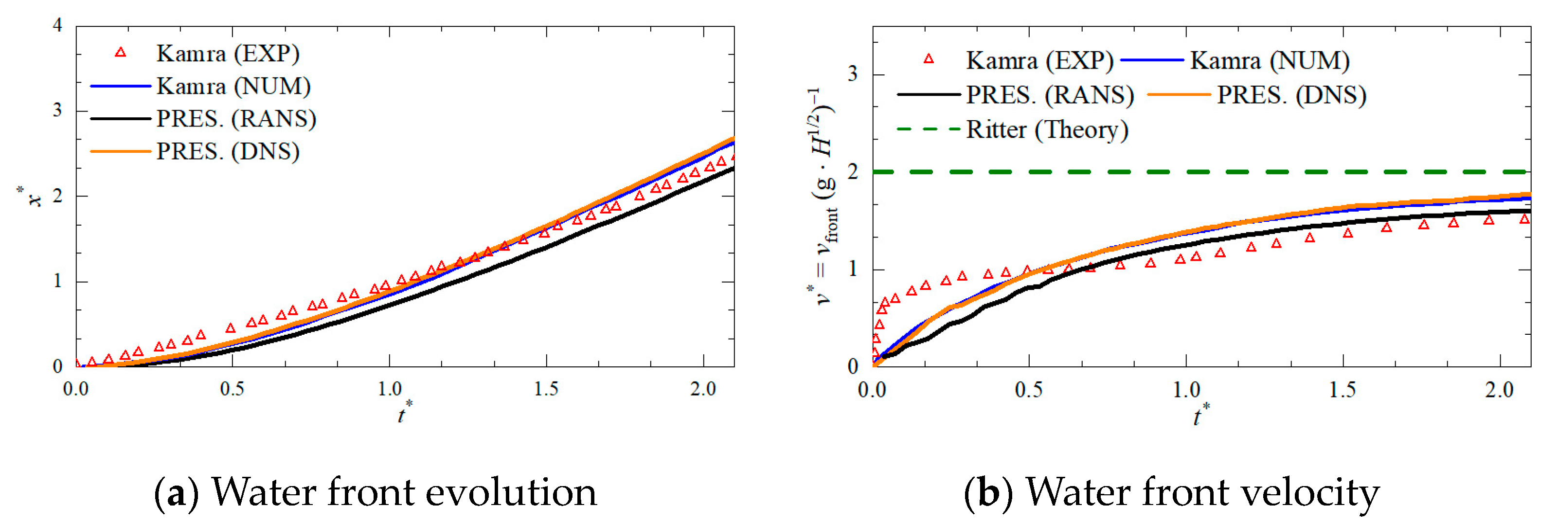
3.3. A Dam-Break Flow Interacting with a Vertical Wall

Figure 5 and Figure 6 show comparisons between the present models (both DNS and RANS) and the published experimental and numerical results in terms of the water front locations and the velocity as well as the pressure time history. The water front velocity is calculated by dividing the traveling distance of the water front (intervals between the measured longitudinal locations) by the travelling time (the corresponding time interval). It can be seen that the RANS model always underestimates the instantaneous positions of the water front measured in the experiments, while the behaviors of the DNS and the numerical model applied in Kamra [49] are relatively more complex. They underestimate the instantaneous locations at the early stage and then overestimate it at a later stage. However, we note that the slopes of all four lines are fairly close to each other (c.f. parallel with each other) at the later stage, i.e., t* > ~1.25. This indicates that the water front velocity before the flow impacting on the wall is captured well by numerical models, as shown in Figure 5b. The discrepancies in the water front evolution and the water front velocity at the early stage may result from the different mechanisms applied for the dam breaking. As mentioned above, in the experiments, this was achieved by opening the gate via a mechanical controlling system. With a careful design, the time duration required for the gate to complete the opening process can be short, i.e., in an order of milliseconds. Even so, the gate-blocking effect is non-negligible. A tiny jet was formed and observed in front of the water column, leading to an increase in the water front velocity at the early stage, as shown in Figure 5b. For reference, the time duration for the gate removal was t* = 0.67 in Ye [21]. After this time instant, i.e., when the gate was fully opened, the water front velocity starts to increase in a steady manner. This trend is well captured by the numerical models. It also can be seen that the analytical solution by the classical dam-break model overestimates the water front velocity. This is due to the fact that the classical dam-break model developed by Ritter [8] assumes a semi-infinite water column and does not consider the bottom friction.
In addition, smaller predictions by the RANS model (when compared to the DNS results) at the earlier stage may result from the use or specification of the initial turbulence intensity (TI), as discussed before. The value of TI = 20% is used in the present RANS model following on Park [26], i.e., no corrections by comparing with the experimental measurements are carried out. A larger initial TI would lead to larger shear stress along the flume bottom, which in turn reduces the water front velocity at the earlier stage. More details about the influence of the initial TI on the dam-break can be found in Park [26].
The main difference between the present CFD models and that in Kamra [49] is the VOF algorithm. Recall that the methodology of isoAdvector is applied in this work, while the free surface is captured by using the unstructured multi-dimensional interface capturing (UMTHINC) scheme in Kamra [49]. The free surface profile is less sensitive to the capturing technique before the impact event when the nonlinearity and deformation of the free surface is small, and hence better agreements between the two models are achieved.
The differences observed in the pressure time history (see Figure 6) mainly lie in the time instant when the impact occurs and the peaks of the pressure. These can also be mainly attributed to the gate motion in the experiments, as discussed before. It is well-recognized that the impact pressure (i.e., the first peak in the time history) is dominated by the water front velocity [53]. As observed in Figure 5a,b and discussed above, the numerical calculated water front velocity is larger than that of the experiments, which in turn leads to an earlier arriving time of the dam-break flow and a larger peak in the impact pressure.
The experimental measurement from Kamra [22] is also included for a direct comparison. The experimental set-ups of the two sets of experiments (i.e., Kamra [22]; Kamra [49]) were similar, although the controlling over the gate motion was slightly different. A small difference in the arriving time between the two experiments was then observed due to this slight difference in the gate motion.
In addition, similar pressure oscillations after the first peak as those in Eijk [54] are observed in the numerical results by the DNS model (see Figure 6). After the initial impact, a small amount of air might be captured to form small air bubbles near the wall corners. Although these bubble volume fractions are relatively small, they cannot escape from both sides in 2D simulations, leading to the large pressure oscillation observed. It is also found that as the mesh is more refined, the oscillation becomes more obvious (results not shown here for brevity). In contrast, the result of the RANS model is relatively smooth. The shape of the water front is blunt in the RANS model, and the aforementioned air pocket is not captured. This is similar to the observations in Park [26]. Nevertheless, the two numerical models established in this work both agree well with the experimental data in terms of the first and the second peak values of the pressure.
As discussed above, the initial TI is required in the RANS-type simulations and plays a significant role in predicting the water front velocity, the impact pressure, etc. The selection of its value has to resort to the experiments. Hence, the DNS-type model is adopted and extended in the subsequent simulations to investigate the dam-break flow with a vertical cylinder of various cross-sections and impacting angles.

3.4. A Dam-Break Flow Interacting with a Vertical Slender Cylinder

Similar numerical setups (including the domain size, boundary conditions, and mesh resolutions, etc.) to those used in Section 3.3 (i.e., a dam-break flow interacting with a vertical wall) are employed here, but now with a vertical cylinder in place. Recall that a pressure sensor was installed for measuring the pressure on the front face of the cylinder in the experiments. This sensor had a diameter of 8 mm, which makes it more suitable for cases with flat surfaces (such as square obstacles and planar walls) and may lead to more measuring uncertainties when mounted on a circular cylinder. For more detailed descriptions, refer to Kamra [22]. The DNS model is also first used for reproducing this set of experiments on the interaction between a dam-break flow and a vertical cylinder for the purpose of validations in this section.

3.4.1. Pressure on the Cylinder

The comparisons in terms of the pressure time history between the present numerical model and the published experiments are carried out in Figure 7. It can be seen that the present numerical model generally overestimates the pressure for both the cylinder cross-sections considered. This is not surprising and is due to the fact that the gate motion is not represented in the numerical simulations, as discussed above. Nevertheless, a satisfactory agreement between the numerical result and the experimental data has been achieved, and thus the applied DNS model can be extended to investigate the dam-break on a slender structure more systematically, as discussed latter in Section 4.
Interestingly, both the DNS model and the experiments capture small pressure variations (i.e., a sudden drop and increase) before or close to the main peak; this is highlighted by the red rectangular box in Figure 7. This may be associated with the shape of the water front or the so-called water tongue. As shown in Figure 8a, the water tongue is analogy to a fluid wedge with an interior angle of a practical value of 40° or less, which is similar to the observations performed by Faltinsen [55] and Greco [56]. More specially, at the beginning of the impact, only a small amount of the fluid at the tip is involved and climbs up the cylinder, forming a thin water sheet along the surface of the cylinder (see Figure 8b). This thin water sheet might act as a cushion for reducing the pressure arising from the further impact of the latter incoming flow. The attack angle of the water tongue would also be altered by the water sheet. From this point of view, only the leading portion of the water hitting the wall can be approximated locally with the half-wedge assumption inherent in the self-similarity solutions (Cumberbatch [11]). As the time increases, the layer of water impacting on the cylinder becomes thicker, with a larger amount of water being involved and more kinetic energy being transferred (see Figure 8c,d). Thus, the pressure is observed to increase again. We note that a higher sampling frequency and a more accurate control over the gate motion are required to capture these pressure variations in the physical experiments. The sampling frequency used in Kamra [22] was 10 kHz, and the output interval for the numerically calculated pressure is 10−7 s, i.e., the sampling frequency is 10,000 kHz in the present numerical simulations.

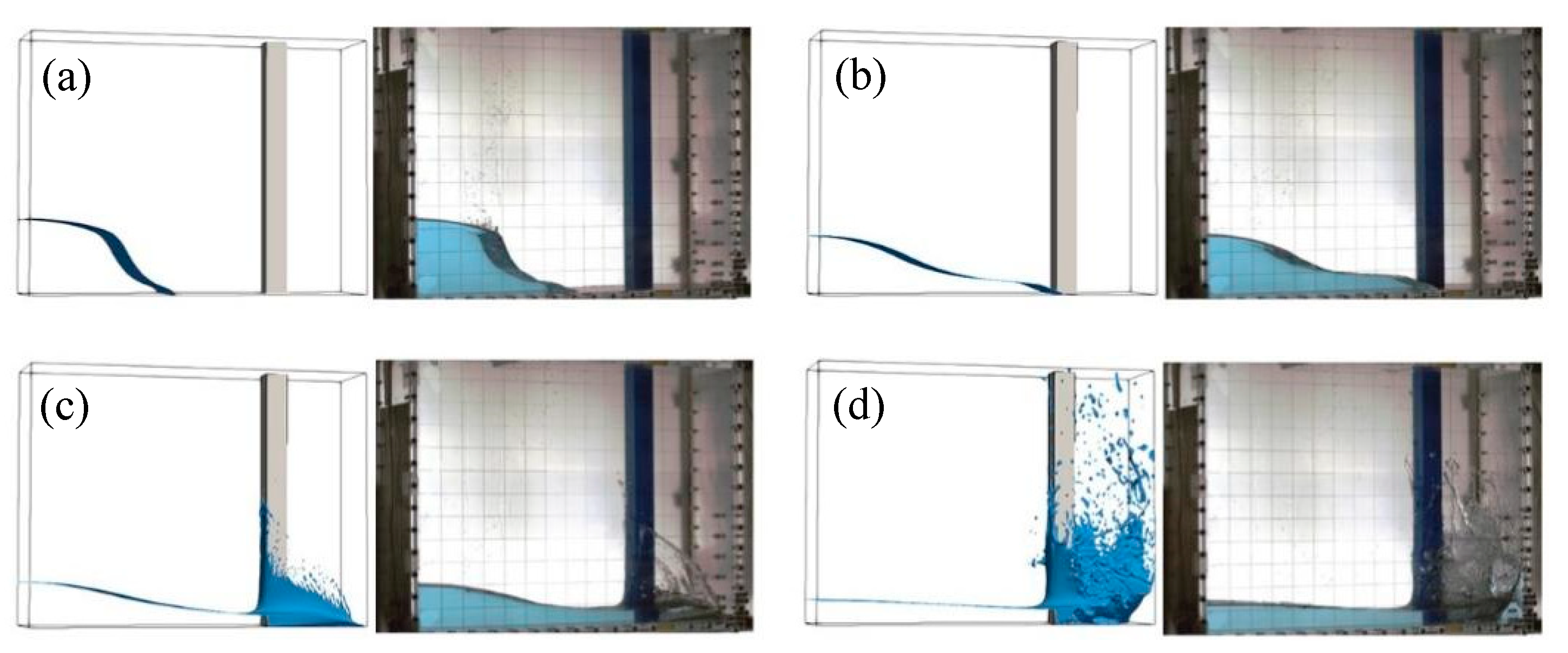
3.4.2. Free Surface Profile

The spatial distributions of the free surface with the cylinder in place at the four typical time instants are shown in Figure 9 (square cylinder) and Figure 10 (circular cylinder). The numerical results are compared with those in the experiments [22]. The free surfaces in the numerical results correspond to the contours of (α = 0.5). The water splashing or spray was observed in the experiments due to the imperfect gate motion (see Figure 9a and Figure 10a). Once the gate is fully open, the dam-break flow travels downstream along the initially dry bed towards the cylinder. The shape of the water tongue is analogous to a half-wedge, as discussed before. At the instant of impact, a violent 3D fluid–structure interaction is expected; part of the water is blocked and climbs up the vertical cylinder and the rest propagates around the cylinder and eventually hits the right flume wall (see Figure 9c and Figure 10c). Then, as shown in Figure 9d and Figure 10d, the water is reflected from the right wall and hit on the back surface of the cylinder, resulting in the negative total longitudinal force on the cylinder, which will be further discussed in Figure 11. In general, the numerical results agree well with the experimental measurements, further confirming the capability of the models applied.
In addition, it can be seen from Figure 9 and Figure 10 that the presence of the cylinders does not affect the free surface profiles before the impacting, while the local flow field around the cylinder and the subsequent reverse impacting from the wall can be rather different. These will be further discussed in the next section.

4. The Effect of the Structural Geometry and the Impacting Angle

It is documented that more than 300 bridges were washed away by the 2011 Great East Japan Tsunami [57]. Not only the pressure on the structure but also the total force resulting from the impact are of concern. As pointed out by Yeh [57], the subsequent impact loading on a cylinder by dam-break should be considered in the early stage of design, including the hydrostatic forces, the buoyant forces, and the hydrodynamic forces. The calculations in terms of the buoyant and hydrostatic forces are relatively straightforward, and thus, in this study, we focus on the hydrodynamic force caused by the frontal impact of the dam-break flow. The effects of the cylinder cross-section and the impacting angle are also explored using the validated numerical models discussed in Section 3.

4.1. The Effect of the Structural Geometry

Time histories of the total longitudinal force on both the circular and the square cylinders are presented in Figure 11. These are results from the DNS model by integrating the pressure over the cylinder surfaces. Here, the force is normalized by ρu2S, where ρ is the density of the water, and u the water front velocity equaling to 2.34 m/s, which is measured just before the impact. S is the area of the vertical cylinder projected in the transverse direction. The pressure variation observed for a vertical cylinder, as the one studied in Figure 7, is not captured here. The tip of the water tongue is too thin to induce a large force/pressure increase [58]. Part of the water that propagates downwards would travel backwards to fill the gap behind the cylinder and eventually impact on the back surface of the cylinder. This results in the negative forces on the square cylinder in the time range of ~(3.2–4.7) and on the circular cylinder in the time range of ~(5.3–6.4), as shown in Figure 11. The impact force arising from the backflow is found to be larger than that of the dam-break flow (i.e., the first peak in the force time history), which is due to the fact that the right wall of the current numerical flume is quite near to the cylinder(s). The water that propagates downwards would impact on the right flume wall first and then be bounced back to form a water jet (red frame in Figure 12a). This water jet hits the square cylinder directly and induces the second impact in Figure 11. However, a similar second impact event does not occur for the circular cylinder due to the violent splashing of the free surface behind the circular cylinder, as shown in Figure 12. The water motions/behaviors become very violent and complex during this process.
In addition, we increase the distance between the cylinder and the right wall to, e.g., 810 mm and 820 mm (the results are not shown here for brevity). It is found that the second impact force induced by the backflow decreases with the increase in this distance, as expected. In addition, this secondary impact is also influenced significantly by the transverse flow field behind the cylinder, i.e., the three-dimensionality of the flow field.
Comparisons between the results of the square and the circular cylinders suggest that the longitudinal force on the latter is smaller than the former (less than 1/2). This is reasonable as nearly all water momentum transfers to the force on the square cylinder due to its flat front surface, i.e., a stagnation zone rather than a stagnation point is formed. While part of flow might be directed sideways from the circular cylinder due to its curved front surface. Hence, the water momentum is not fully transferred, resulting in a smaller force on the cylinder even when the (projected) impacting area is the same.

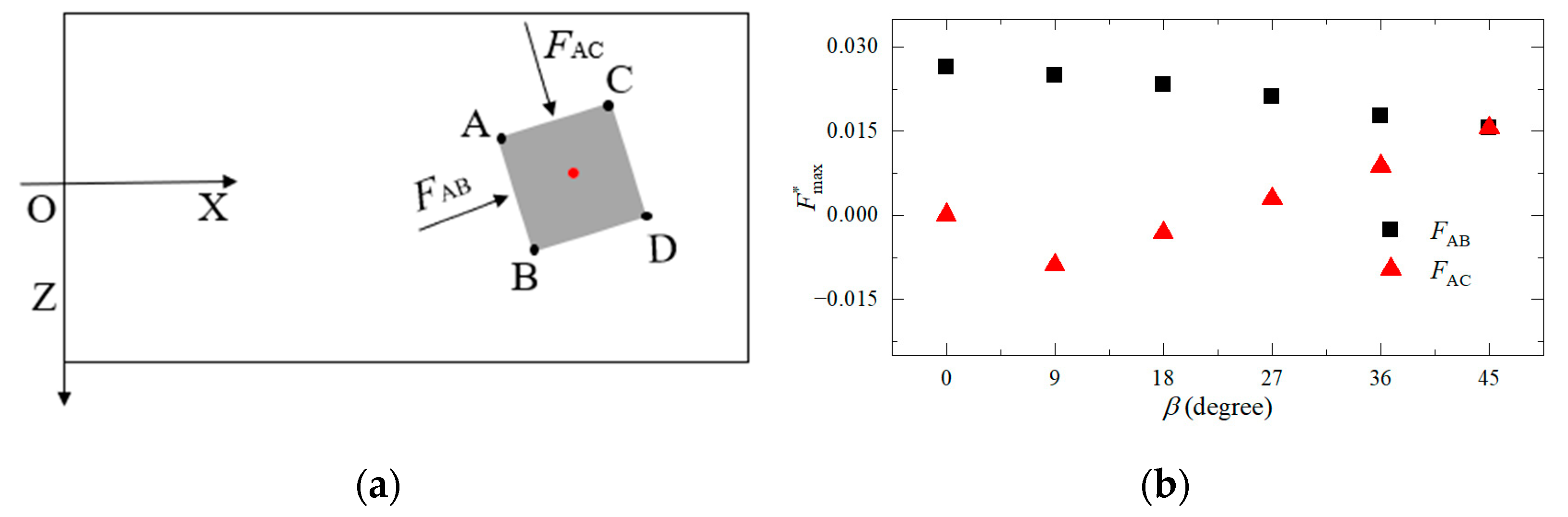
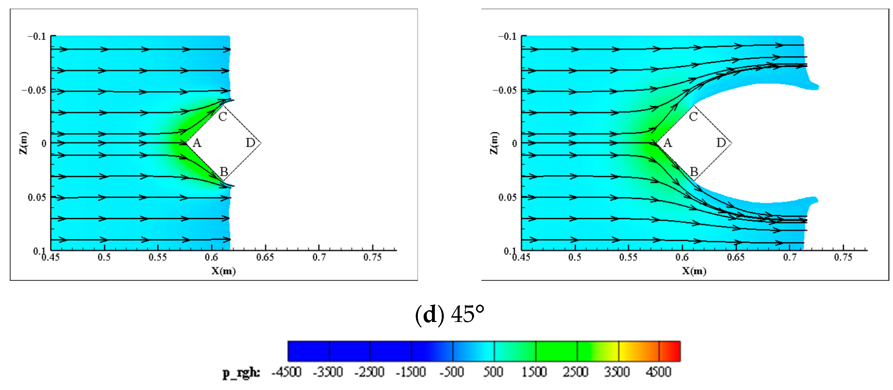
4.2. The Effect of the Impacting Angle

As mentioned above, more violent and complex behaviors would be induced when the dam-break flow reaches and is reflected by the right flume wall, accompanied with the violent splashing of the free surface. Hence, the length of the domain in this section is increased to 975 mm, as discussed in Section 3. This is reasonable as we focus on the loading by a forward-moving dam-break flow. We also note here that only a square cylinder is considered as the circular cylinder is axially symmetric.
The maximum total longitudinal and transverse forces on the square cylinder caused by the first impact are shown in Figure 13, in which various impacting angles are considered. Here, the force normalization is the same as in the former Section (i.e., ρu2S, where ρ is the density of the water; u = 2.34 m/s is the water front velocity before the impact; and S is the area of the vertical cylinder projected in the longitudinal and transverse direction, respectively). It can be seen that the maximum longitudinal force decreases with the impacting angle monotonously, while the maximum transverse force increases first with the impacting angle to its maximum value at β = ~18° and then decreases with its further increase. The direction of the transverse force is always pointing towards the negative Z-axis, and it is found that the maximum transverse force is nearly half of the maximum longitudinal force at ~18° < β <~27°.
The free surface profiles (looking from different directions) at the time instant when the maximum longitudinal force is achieved are shown in Figure 14. It is noted that the value of this time instant, i.e., occurrence of impact, can be slightly different for cases with different impacting angles. It can be seen that the dam-break flow separates at the front edge/corner(s) of the square cylinder. The water is more flexible (i.e., less violent) when flowing around the cylinder if there is a clear flow separation region in front of the cylinder [34]. This explains why the maximum longitudinal force decreases with the impacting angle, as observed in Figure 13.
It is also clear from Figure 14 that, as the dam-break bore strikes the square cylinder, a large amount of water is forced to run-up along the vertical cylinder. For oblique attacks of β = 9° and 36°, more water is observed to run-up along Face AB when compared to Face AC. The asymmetry of the local flow field is remarkable, leading to the relatively larger transverse force in Figure 13. Note that the illustration of Face AB and Face AC can be found on the top left of Figure 14a. While for 0° and 45°, the flow is directed symmetrically along the front edge of the square cylinder, and hence the transverse forces are nearly equal to zero (the transverse forces on the two symmetric faces are cancelled out). This phenomenon differs from the observations in the physical experiments by Yeh [34] and the SPH-based (smoothed particle hydrodynamics) numerical simulations by Wei [52]. They considered the so-called wet-deck dam-break in which a high turbulent dam-break flow/bore was generated and plunged into a (very) shallow water, and then propagated downwards to hit on a square cylinder. This chaotic turbulence results in the asymmetry of the flow field even when the structure is symmetric. For the present study, the so-called dry-deck dam-break model is applied, in which the flume bottom is initially dry. As discussed before, the turbulence effect is negligible for this type of problem, thus the free surface profile is expected to be symmetric when the structure is symmetric.
The maximum forces on Face AB (FAB) and Face AC (FAC) at various impacting angles are then shown in Figure 15, together with a sketch highlighting their directions. It can be seen that the maximum FAB is always larger than the maximum FAC, and this decreases with the impacting angle. In addition, it is found that the direction of FAB always points towards Face AB for the cases considered. However, the force on Face AC points outwards at β < ~27°, and its value increases with the impacting angle in the range of (9°–27°). This negative characteristic can be well explained by the excessive pressure fields at Y = 0.001 m shown in Figure 16. The left-hand side of Figure 16 shows the results at t* = 1.5, which can be considered the initial stage of the impact, and the right-hand side shows the results at t* = 2.03. It can be seen that for the case with an impacting angle of 9° (the second row of Figure 16), there is an obvious negative pressure region formed initially at an area close to corner A, which then develops and propagates downwards. This results in the negative force observed in Figure 15, and the results from the flow separation at corner A; a small amount of water flow is reversed to fill the gap behind the separation point. We note here that this negative pressure region also exists for the cases with an impacting angle ~0° < β < ~27° but less violent, and hence leading to a smaller negative force.
In addition, it is also interesting to analyze the flow separation behaviors with the aid of flow visualization (one of main advantages of the CFD-based numerical simulations). It can be seen that obvious stagnation regions emerge in front of the square cylinder, which induce pressure increases in this region. For 0° and 9°, the increased pressure region is in front of Face AB and vanishes at separation points A and B. The stagnation points of them are at the middle of Face AB and the left corner (facing downstream) near point A, respectively. For 27° and 45°, Face AB and Face AC are wrapped by the increased pressure region, and the stagnation points are both close to point A.
The flow separates at points A and B for the case with an impacting angle of 0°, which is consistent to the observations by Yen and Yang [59] (see Figure 16a). In Yen and Yang [59], a uniform flow propagating around a square cylinder was considered. However, the flow separation near the rear of the cylinder is not formed because a transient rather than a steady process is considered in this work.
The situation is however rather different at 9°. As discussed, there is a negative pressure region close to the corner of point A. A small reverse flow is formed here by the adverse pressure gradient. A counterclockwise separation bubble and the negative pressure region are amplified gradually along Face AC. This region moves along AC and reattaches on Face AC at X = 0.6 m.
For 27° and 45°, the flow separation demonstrates a smooth streamline without forming a reverse flow, and thus the water moves downstream along Face AB and AC. With the development of the flow, the water ultimately separates at Points B and C, and the flow bifurcates into two streams propagating downstream from both sides. It is worth noting that there is no interference on Faces BD and CD until the maximum force is obtained for the cases considered.

5. Conclusions

A CFD-type model based on OpenFOAM has been established and is extended to study the interaction between a dam-break flow and a vertical circular and square cylinder. This is helpful for investigating the greenwater impact or the tsunami landing. A good agreement between the numerical results (both DNS and RANS) and the corresponding experimental data is obtained, which indicates that the present model works well for resolving such problems by overcoming the various assumptions used in the shallow water equations or the potential flow theory to a certain extent. The validated model is then used for investigating the effect of the structural geometry and the impacting angle, and the local flow field around the cylinder is also detailed. We note that the DNS model is utilized for these further investigations as the accuracy of the RANS model is highly dependent on the initial TI that is prescribed empirically and is corrected iteratively by comparing with the experimental measurements.
The water tongue that has a half-wedge-like shape is well captured in this work and is found to have a significant influence on the pressure oscillation during the initial stage of the impact on vertical cylinders. The total longitudinal force on the square cylinder is twice that of the circular cylinder with the same impacting area. Nearly all the water momentum is transferred to the impact force due to the flat front surface of the square cylinder.
Water that travels around the cylinder downstream hits the right flume wall and then travels backwards to impact the back surface of the cylinder. This results in significant negative forces on the cylinder (even larger than the impact load by the forward-moving dam-break flow). This is nontrivial and helpful in arranging the layout of, e.g., on-deck structures of an FPSO.
In addition, the impact forces are found to decrease with the impacting angle in the longitudinal direction, and the transverse loads are induced if the square cylinder is not symmetric around the flow centerline. The transverse forces increase first with the impacting angle when β < ~18° and then decrease with a further increase in the impacting angle.
The free surface profile and the excessive pressure field at typical time instants are also shown to help with explaining the related mechanism. Different separation modes during the first impact event are observed at different impacting angles. A violent negative pressure region is formed at smaller impacting angles (less than 27°), leading to the force pointing outward from the structure face.

Author Contributions

Conceptualization, D.M., L.C. and D.N.; data curation, D.M.; formal analysis, D.M.; funding acquisition, L.C.; investigation, D.M.; methodology, L.C. and D.N.; project administration, L.C.; resources, D.N.; software, D.M.; supervision, L.C. and D.N.; validation, D.M.; visualization, D.M.; writing—original draft, D.M.; writing—review and editing, L.C. and D.N. All authors have read and agreed to the published version of the manuscript.

Funding

This work is supported by the National Natural Science Foundation of China (Grant No. 52001053) and the Natural Science Foundation of Liaoning Province (Grant No. 2021-KF-16-03).

Data Availability Statement

The data that support the findings of this study are available from the corresponding authors upon reasonable request.

Conflicts of Interest

The authors declare no conflict of interest.

References

  1. Stansby, P.K.; Chegini, A.; Barnes, T.C.D. The initial stages of dam-break flow. J. Fluid Mech. 1998, 374, 407–424. [Google Scholar] [CrossRef]
  2. Li, Y.L.; Ma, Y.; Deng, R.; Jiang, D.P.; Hu, Z. Research on dam-break induced tsunami bore acting on the triangular breakwater based on high order 3D CLSVOF-THINC/WLIC-IBM approaching. Ocean. Eng. 2019, 182, 645–659. [Google Scholar] [CrossRef]
  3. Stoker, J.J. Water Waves: The Mathematical Theory with Applications; Interscience: New York, NY, USA, 1957. [Google Scholar]
  4. Kawashima, K.; Buckle, I. Structural performance of bridges in the tohoku-oki earthquake. Earthq. Spectra 2013, 29, S315–S338. [Google Scholar] [CrossRef]
  5. Health and Safety Executive (HSE). Findings of an Expert Panel Engaged to Conduct a Scoping Study on Survival Design of Floating Production Storage and Offloading Vessels against Extreme Ocean Conditions; Research Report; No 357; Health and Safety Executive (HSE): Merseyside, UK, 2005.
  6. Hogg, A.J.; Woods, A.W. The transition from inertia- to bottom-drag-dominated motion of turbulent gravity currents. J. Fluid Mech. 2001, 449, 201–224. [Google Scholar] [CrossRef]
  7. Hogg, A.J.; Pritchard, D. The effects of hydraulic resistance on dam-break and other shallow inertial flows. J. Fluid Mech. 2004, 501, 179–212. [Google Scholar] [CrossRef]
  8. Ritter, A. Die fortpflanzung der wasserwellen zeitschrift des vereins. Dtsch. Ing. Zeitswchrift 1982, 36, 947–954. [Google Scholar]
  9. Ungarish, M. A simple model for the reflection by a vertical barrier of a dambreak flow over a dry or pre-wetted bottom. J. Fluid Mech. 2022, 942, R6. [Google Scholar] [CrossRef]
  10. Wang, B.; Liu, X.; Zhang, J.M. Analytical and Experimental Investigations of Dam-Break Flows in Triangular Channels with Wet-Bed Conditions. J. Hydraul. Eng. 2020, 146, 04020070. [Google Scholar] [CrossRef]
  11. Cumberbatch, E. The impact of a water wedge on a wall. J. Fluid Mech. 1960, 7, 353–374. [Google Scholar] [CrossRef]
  12. Cross, R.H. Tsunami surge forces. J. Waterw. Harb. Div. 1967, 93, 201–231. [Google Scholar] [CrossRef]
  13. Kihara, N.; Niida, Y.; Takabatake, D.; Kaida, H.; Shibayama, A.; Miyagawa, Y. Large-scale experiments on tsunami-induced pressure on a vertical tide wall. Coast. Eng. 2015, 99, 46–63. [Google Scholar] [CrossRef]
  14. Raju, K.G.R.; Asawa, G.L.; Rana, O.P.S.; Pillai, A.S.N. Rational assessment of blockage effect in channel flow past smooth circular-cylinders. J. Hydraul. Res. 1983, 21, 289–302. [Google Scholar] [CrossRef]
  15. Qi, Z.X.; Eames, I.; Johnson, E.R. Force acting on a square cylinder fixed in a free-surface channel flow. J. Fluid Mech. 2014, 756, 716–727. [Google Scholar] [CrossRef]
  16. Vosoughi, F.; Nikoo, M.R.; Rakhshanderhroo, G. Downstream semi-circular obstacles’ influence on floods arising from the failure of dams with different levels of reservoir silting. Phys. Fluids 2022, 34, 013312. [Google Scholar] [CrossRef]
  17. Liu, W.J.; Wang, B.; Guo, Y.K.; Zhang, J.M.; Chen, Y.L. Experimental investigation on the effects of bed slope and tailwater on dam-break flows. J. Hydrol. 2020, 590, 125256. [Google Scholar] [CrossRef]
  18. Kleefsman, K.M.T.; Fekken, G.; Veldman, A.E.P.; Iwanowski, B.; Buchner, B. A volume-of-fluid based simulation method for wave impact problems. J. Comput. Phys. 2005, 206, 363–393. [Google Scholar] [CrossRef]
  19. Lobovsky, L.; Botia-Vera, E.; Castellana, F.; Mas-Soler, J.; Souto-Iglesias, A. Experimental investigation of dynamic pressure loads during dam break. J. Fluids Struct. 2014, 48, 407–434. [Google Scholar] [CrossRef]
  20. Rajaie, M.; Azimi, A.H.; Nistor, I.; Rennie, C.D. Experimental Investigations on Hydrodynamic Characteristics of Tsunami-Like Hydraulic Bores Impacting a Square Structure. J. Hydraul. Eng. 2022, 148, 04021061. [Google Scholar] [CrossRef]
  21. Ye, Z.T.; Zhao, X.Z.; Deng, Z.Z. Numerical investigation of the gate motion effect on a dam break flow. J. Mar. Sci. Technol. 2016, 21, 579–591. [Google Scholar] [CrossRef]
  22. Kamra, M.M.; Al Salami, J.; Sueyoshi, M.; Hu, C.H. Experimental study of the interaction of dam break with a vertical cylinder. J. Fluids Struct. 2019, 86, 185–199. [Google Scholar] [CrossRef]
  23. Liu, W.J.; Wang, B.; Guo, Y.K. Numerical study of the dam-break waves and Favre waves down sloped wet rigid-bed at laboratory scale. J. Hydrol. 2021, 602, 126752. [Google Scholar] [CrossRef]
  24. McLoone, M.; Quinlan, N.J. Particle transport velocity correction for the finite volume particle method for multi-resolution particle distributions and exact geometric boundaries. Eng. Anal. Bound. Elem. 2020, 114, 114–126. [Google Scholar] [CrossRef]
  25. Park, I.R.; Kim, K.S.; Kim, J.; Van, S.H. A volume-of-fluid method for incompressible free surface flows. Int. J. Numer. Methods Fluids 2009, 61, 1331–1362. [Google Scholar] [CrossRef]
  26. Park, I.R.; Kim, K.S.; Kim, J.; Van, S.H. Numerical investigation of the effects of turbulence intensity on dam-break flows. Ocean. Eng. 2012, 42, 176–187. [Google Scholar] [CrossRef]
  27. Facci, A.L.; Ubertini, S. Numerical assessment of similitude parameters and dimensional analysis for water entry problems. Math. Probl. Eng. 2015, 2015, 324961. [Google Scholar] [CrossRef]
  28. Reddy, D.N.; Scanlon, T.J.; Kuo, C. Prediction of slam loads on a wedge section using computational fluid dynamics (CFD) techniques. In Proceedings of the Twenty-Fourth Symposium on Naval Hydrodynamics, Fukuoka, Japan, 8–13 July 2002. [Google Scholar]
  29. Seng, S.; Jensen, J.J.; Pedersen, P.T. Numerical prediction of slamming loads. J. Eng. Marit. Environ. 2012, 226, 120–134. [Google Scholar] [CrossRef]
  30. Hu, C.H.; Kashiwagi, M. A CIP-based method for numerical simulations of violent free-surface flows. J. Mar. Sci. Technol. 2004, 9, 143–157. [Google Scholar] [CrossRef]
  31. Zhao, H.Y.; Ming, P.J.; Zhang, W.P.; Chen, J.K. A direct time-integral THINC scheme for sharp interfaces. J. Comput. Phys. 2019, 393, 139–161. [Google Scholar] [CrossRef]
  32. Violeau, D.; Issa, R. Numerical modelling of complex turbulent free-surface flows with the SPH method: An overview. Int. J. Numer. Methods Fluids 2007, 53, 277–304. [Google Scholar] [CrossRef]
  33. Wu, T.-R.; Liu, P. Numerical study on the three-dimensional dam-break bore interacting with a square cylinder. In Nonlinear Wave Dynamics: Selected Papers of the Symposium Held in Honor of Philip L-F Liu’s 60th Birthday; World Scientific: Singapore, 2009; pp. 281–303. [Google Scholar]
  34. Yeh, H.; Shuto, N. Tsunami forces and effects on structures. J. Disaster Res. 2009, 4, 375–376. [Google Scholar] [CrossRef]
  35. Duan, L.L.; Zhu, L.; Chen, M.S.; Pedersen, P.T. Experimental study on the propagation characteristics of the slamming pressures. Ocean. Eng. 2020, 217, 107868. [Google Scholar] [CrossRef]
  36. Brown, S.A.; Greaves, D.M.; Magar, V.; Conley, D.C. Evaluation of turbulence closure models under spilling and plunging breakers in the surf zone. Coast. Eng. 2016, 114, 177–193. [Google Scholar] [CrossRef]
  37. Launder, B.E.; Spalding, D.B. The numerical computation of turbulent flows. Comput. Methods Appl. Mech. Eng. 1974, 3, 269–289. [Google Scholar] [CrossRef]
  38. Lakshman, R.; Binod, J.R.; Basak, R. Implementation of improved wall function for buffer sub-layer in OpenFOAM. In Proceedings of the International Conference on Thermofluids, Video, 10–11 November 2021; Springer: Singapore, 2021; pp. 61–69. [Google Scholar]
  39. Hirt, C.W.; Nichols, B.D. Volume of fluid (VOF) method for the dynamics of free boundaries. J. Comput. Phys. 1981, 39, 201–225. [Google Scholar] [CrossRef]
  40. Biscarini, C.; Francesco, S.D.; Manciola, P. CFD modelling approach for dam break flow studies. Hydrol. Earth Syst. Sci. 2010, 14, 705–718. [Google Scholar] [CrossRef]
  41. Zhang, X.T.; Tian, X.; Guo, X.; Li, X.; Xiao, L. Bottom step enlarging horizontal momentum flux of dam break flow. Ocean. Eng. 2020, 214, 107729. [Google Scholar] [CrossRef]
  42. Audusse, E.; Benkhaldoun, F.; Sari, S.; Seaid, M.; Tassi, P. A fast finite volume solver for multi-layered shallow water flows with mass exchange. J. Comput. Phys. 2014, 272, 23–45. [Google Scholar] [CrossRef]
  43. Kocaman, S.; Ozmen-Cagatay, H. Investigation of dam-break induced shock waves impact on a vertical wall. J. Hydrol. 2015, 525, 1–12. [Google Scholar] [CrossRef]
  44. Roenby, J.; Bredmose, H.; Jasak, H. A computational method for sharp interface advection. R. Soc. Open Sci. 2016, 3, 160405. [Google Scholar] [CrossRef] [PubMed]
  45. Scheufler, H.; Roenby, J. Accurate and efficient surface reconstruction from volume fraction data on general meshes. J. Comput. Phys. 2019, 383, 1–23. [Google Scholar] [CrossRef]
  46. Courant, R.; Friedrichs, K.; Lewy, H. On the partial difference equations of mathematical physics. IBM J. Res. Dev. 1967, 11, 215–234. [Google Scholar] [CrossRef]
  47. Harten, A. High-resolution schemes for hyperbolic conservation-laws. J. Comput. Phys. 1983, 49, 357–393. [Google Scholar] [CrossRef]
  48. Issa, R.I. Solution of the implicitly discretized fluid-flow equations by operator-splitting. J. Comput. Phys. 1986, 62, 40–65. [Google Scholar] [CrossRef]
  49. Kamra, M.M.; Mohd, N.; Liu, C.; Sueyoshi, M.; Hu, C.H. Numerical and experimental investigation of three-dimensionality in the dam-break flow against a vertical wall. J. Hydrodyn. 2018, 30, 682–693. [Google Scholar] [CrossRef]
  50. Sueyoshi, M.; Hu, C. Experimental technique and particle simulation for large deformation problems of free-surface. In Conference Proceedings of Japan Society of Naval Architects and Ocean Engineers; Japan Society of Naval Architects and Ocean Engineers: Tokyo, Japan, 2015; pp. 93–94. [Google Scholar]
  51. Buchner, B. Green Water on Ship-Type Offshore Structures. Ph.D. Thesis, Delft University of Technology, Delft, The Netherlands, 2002. [Google Scholar]
  52. Wei, Z.P.; Dalrymple, R.A.; Hérault, A.; Bilotta, G.; Rustico, E.; Yeh, H. SPH modeling of dynamic impact of tsunami bore on bridge piers. Coast. Eng. 2015, 104, 26–42. [Google Scholar] [CrossRef]
  53. Greco, M.; Faltinsen, O.M.; Landrini, M. Shipping of water on a two-dimensional structure. J. Fluid Mech. 2005, 525, 309–332. [Google Scholar] [CrossRef]
  54. Eijk, M.; Wellens, P.R.; Bos, R.W. Aerated wave impacts on floating bodies. In Proceedings of the Thirty-Fifth International Workshop on Water Waves and Floating Bodies, Seoul, Republic of Korea, 24–27 August 2020. [Google Scholar]
  55. Faltinsen, O.M.; Landrini, M.; Greco, M. Slamming in marine applications. J. Eng. Math. 2004, 48, 187–217. [Google Scholar] [CrossRef]
  56. Greco, M. A Two-Dimensional Study of Green-Water Loading. Ph.D. Thesis, Norwegian University of Science and Technology, Trondheim, Norway, 2001. [Google Scholar]
  57. Yeh, H. Design tsunami forces for onshore structures. J. Disaster Res. 2007, 2, 531–536. [Google Scholar] [CrossRef]
  58. Ramsden, J.D. Tsunamis: Forces on a Vertical Wall Caused by Long Waves, Bores, and Surges on a Dry Bed; California Institute of Technology: Pasadena, CA, USA, 1993. [Google Scholar]
  59. Yen, S.C.; Yang, C.W. Flow patterns and vortex shedding behavior behind a square cylinder. J. Wind. Eng. Ind. Aerodyn. 2011, 99, 868–878. [Google Scholar] [CrossRef]
Figure 1. A dam-break flow, incurred by collapsing the water volume at the left corner, interacting with a vertical wall represented by the flume end in the opposite direction.
Jmse 11 00932 g001
Figure 2. A dam-break flow interacting with a vertical cylinder of finite size. The cross-section of the cylinder is either circular or square, and its diameter and side length are the same; both equal to 50 mm. (a) The three-dimensional perspective; (b) the top view showing the definition of the impacting angle (β), the cylinder projected width along Z-axis (w′), and the length between the cylinder center and the right wall (l′).
Jmse 11 00932 g002
Figure 3. (a) Front view of the computational domain; (b) the mesh topology at the right corner.
Jmse 11 00932 g003
Figure 4. (a) Variations in the longitudinal location of the water front with the time; (b) the spatial profile of the water surface at t* = 5.6.
Jmse 11 00932 g004
Figure 5. The comparisons of water front evolution and velocity among the present numerical results and the theorical [8], the published experimental [49] as well as numerical results [49].
Jmse 11 00932 g005
Figure 6. The comparisons of pressure time history among the present numerical results and the published experimental (EXP 2018 and 2019 refer to [49] and [22], respectively) as well as numerical results [49].
Jmse 11 00932 g006
Figure 7. Comparisons of the pressure time history provided by the present numerical model and the published experiments [22]. The time is shifted so that the impacting time, i.e., the occurrence of the first peak, equals zero.
Jmse 11 00932 g007
Figure 8. The slice (Z = 0 m) of the flow field and the streamlines (black lines with arrows) in front of the square cylinder during the first impact event.
Jmse 11 00932 g008
Figure 9. Spatial distributions of the free surface at the four typical time instants for the case with the square cylinder. (a) The initial stage (t* = 1.05); (b) the first impact event on the cylinder (t* = 1.75); (c) the impact on the right vertical wall (t* = 2.45); (d) the impact event on the cylinder by the reverse flow (t* = 3.5). Left subplot represents the CFD results and right the experimental photos.
Jmse 11 00932 g009
Figure 10. Spatial distributions of the free surface at the four typical time instants for the case with the circular cylinder. (a) The initial stage (t* = 1.05); (b) the first impact event on the cylinder (t* = 1.75); (c) the impact on the right vertical wall (t* = 2.45); (d) the impact event on the cylinder by the reverse flow (t* = 3.5). Left subplot represents the CFD results and right the experimental photos.
Jmse 11 00932 g010
Figure 11. Time history of the longitudinal force on the cylinder provided by the DNS model.
Jmse 11 00932 g011
Figure 12. Top view of the flow field at t* = 3 (second impact).
Jmse 11 00932 g012
Figure 13. The maximum longitudinal and transverse forces on the square cylinder.
Jmse 11 00932 g013
Figure 14. The free surface profile (α = 0.5; looking from three different directions) around the square cylinder at the time instant when the maximum longitudinal force is achieved.
Jmse 11 00932 g014aJmse 11 00932 g014b
Figure 15. (a) The sketch of the force directions; (b) the maximum forces on Face AB and Face AC.
Jmse 11 00932 g015
Figure 16. The excessive pressure field at Y = 0.001 m (the streamline and flow direction are presented by black lines) at the two typical time instants. (Left): initial stage (t* = 1.5); (right): t* = 2.03.
Jmse 11 00932 g016aJmse 11 00932 g016b
Table 1. Physical properties of the two fluids considered.
Physical PropertiesWaterAir
Density (kg/m3)999.71.2
Molecular viscosity (kg/(m·s))1.307 × 10−31.4 × 10−5
Surface tension coefficient (N/m)0.0742
Table 2. Mesh parameters and the total cell number.
SpacingCoarseMediumFine
ΔminH/800H/1500H/2500
ΔmaxH/80H/150H/250
Total number120 k258 k811 k
Cores number161632
Computational time (s)1596458474
Disclaimer/Publisher’s Note: The statements, opinions and data contained in all publications are solely those of the individual author(s) and contributor(s) and not of MDPI and/or the editor(s). MDPI and/or the editor(s) disclaim responsibility for any injury to people or property resulting from any ideas, methods, instructions or products referred to in the content.

