An Approach for Shipping Emissions Estimation in Ports: The Case of Ro–Ro Vessels in Port of Vigo

Abstract

Despite most atmospheric emissions being produced by vessels when navigating at sea, they are also important when in port because of their proximity to urban areas and their harmful effects on climate change and health. First, we carried out a bibliographical review of the nine most relevant methods to estimate the emission of ships in ports. These methods have been used to estimate the emissions of the sixteen most representatives Ro–Ro (roll-on–roll-off) ships calling at the Port of Vigo. From the results obtained, a new simplified method for estimation is proposed, which is based on linear regression curves and takes into account the number of ships and the average number of hours they remain in port annually. This simplification could be a useful tool when making preliminary assessments of the emissions from ships in port, which can also be extrapolated to other ports or types of ships.

1. Introduction

Atmospheric emissions from ships during a voyage come mainly from their main engines [1]. While in port, however, they mainly come from the auxiliary engines (AE), which are used to produce power in loading, unloading and hoteling operations [2,3,4,5].

Although the quantity of emissions during this port stage is lower than during the voyage stage, the environmental pollution directly affects nearby population centers [6].

Carbon dioxide (CO₂) is the most important pollutant regarding greenhouse gas (GHG) emissions. However, special attention should also be paid to the presence of other atmospheric pollutants in port cities due to their impact on human health [7,8]: particulate matter (PM), volatile organic compounds (VOCs), carbon monoxide (CO), nitrogen oxides (NO_x) and sulfur oxides (SO_x).

According to the European Maritime Safety Agency (EMSA) report for 2021 [9], the most important emissions from ships stopping in ports in the European Union (EU) or in the European Economic Area were CO₂ (

Table 1. Emissions by pollutant (t) of vessels calling at EU ports (2018–2019) [9].

Pollutant Type	Emissions (106 t)
CO2	140
SO2	1.63
NO2	4.46
PM2.5	0.26

). Furthermore, around 40% were produced by voyages between ports of EU Member States, this being 6% when ships are at berth.

There is a great need for analyses of emissions from ships during their stay in ports and also for the establishment of measures to reduce them; according to some studies [7,8,9]:

• A total of 70% of ship emissions are estimated to occur within 400 km of land;
• A total of 90% of European ports are spatially connected to cities;
• The harmful effects of these pollutants affect almost 40% of the European population, who live within 50 km of the sea.

For these reasons, the norms on controlling ship emissions in port are increasingly restrictive:

• Internationally, they are regulated by Annex VI of the MARPOL Convention “Prevention of Air Pollution from Ships” added to the 1997 Protocol of the International Maritime Organization (IMO). This establishes a progressive reduction in SO_x, NO_x, and PM emissions and the introduction of emission control areas (ECAs) [10]. Amendments to this Annex VI were carried out in 2021 in order to reduce de GHG emissions from ships. These amendments require ships to improve their energy efficiency to reduce their emissions. From 1 January 2023 it is mandatory for all ships to calculate their attained Energy Efficiency Existing Ship Index (EEXI) to measure their energy efficiency and to initiate the collection of data for the reporting of their annual operational carbon intensity indicator (CII) and CII rating [11].
• At a European level, Directive (UE) 2016/802 [12] sets the reduction in the sulfur content of certain liquid fuels. More specifically, Article 7 sets a limit of 0.1% of sulfur content by mass for marine fuels used by ships in port, unless they are berthed for less than two hours or they switch off all their engines because they are connected to the shore-side electricity supply. With respect to greenhouse gas emissions, Regulation (UE) 2015/757 [13] established the monitoring, reporting and verification of carbon dioxide emissions from maritime transport. However, the biggest commitment of the European Union was adopted from 2019 with the European Green Deal [14] developed by European Climate Law [15] and the package of proposals ‘Fit for 55′ [16] in 2021. These documents have set ambitious targets for reducing net emissions by at least 55% by 2030 compared to 1990 and for achieving the climate neutral by 2050. These proposes include the maritime sector in an emissions trading scheme and develop the Fuel EU Maritime initiative, which aims to increase the demand for use of renewable and low-carbon fuels and reduce their greenhouse gas emissions.

Therefore, these norms limit the type of fuel used in ships and also their engines, which also has repercussions on consumption and pollutant emissions.

For example, these parameters are essential for:

• Analyzing any emissions reduction measure;
• Simulating the dispersion of air pollution [17];
• Introducing new fuels with low or zero sulfur content (liquid natural gas, methane–methanol, hydrogen, and ammonia) and incorporating batteries and renewable systems in ships [18,19];
• Supplying electricity to the ship in port [20] (through an electrical micro-grid that can manage renewable energy production, the use of fuel cells and batteries and supply from the electricity grid;
• Implementing a Smart Port [21].

Emissions from ships can currently be estimated by:

• Data that the Automatic Identification System (AIS) transmits on each ship: IMO identification number, size, weight, name, type, position, speed, heading, etc. This system was passed by the IMO in 2002 and is mandatory on ships covered by the Convention of Safety of Life at Sea (SOLAS) to improve safety and efficiency of navigation [7];
• Technical information obtained from the IT database of Lloyd’s Register of Shipping (LRS), port authorities’ databases, engine ship manufacturers, ship owners, etc. [22].

This article aims to undertake a bibliographical review of the various methods existing to estimate the emissions from ships in port in order to:

• Analyze and compare the different methodologies used in the calculation of emissions from ships during their stay in port, through the analysis of a specific case corresponding to the Ro–Ro ships that call at the Port of Vigo. These ships were selected because of their importance for this port in cargo traffic [23], and because the number of hours of Ro–Ro ships stayed in 2018 was about 16 times higher than those for transatlantic vessels [24,25];
• Establish a simplified calculation of emissions from ships in port.

2. Methodology

This section contains the most relevant methods to estimate emissions from ships during their stay in ports taken from the bibliographical review undertaken.

These emissions can be obtained from the power of the ship’s auxiliary engines or from fuel consumption. As this information is not generally available, it is estimated from the gross tonnage (GT), usually by using regression curves [4,5]. This GT parameter is freely accessible on several shipping websites.

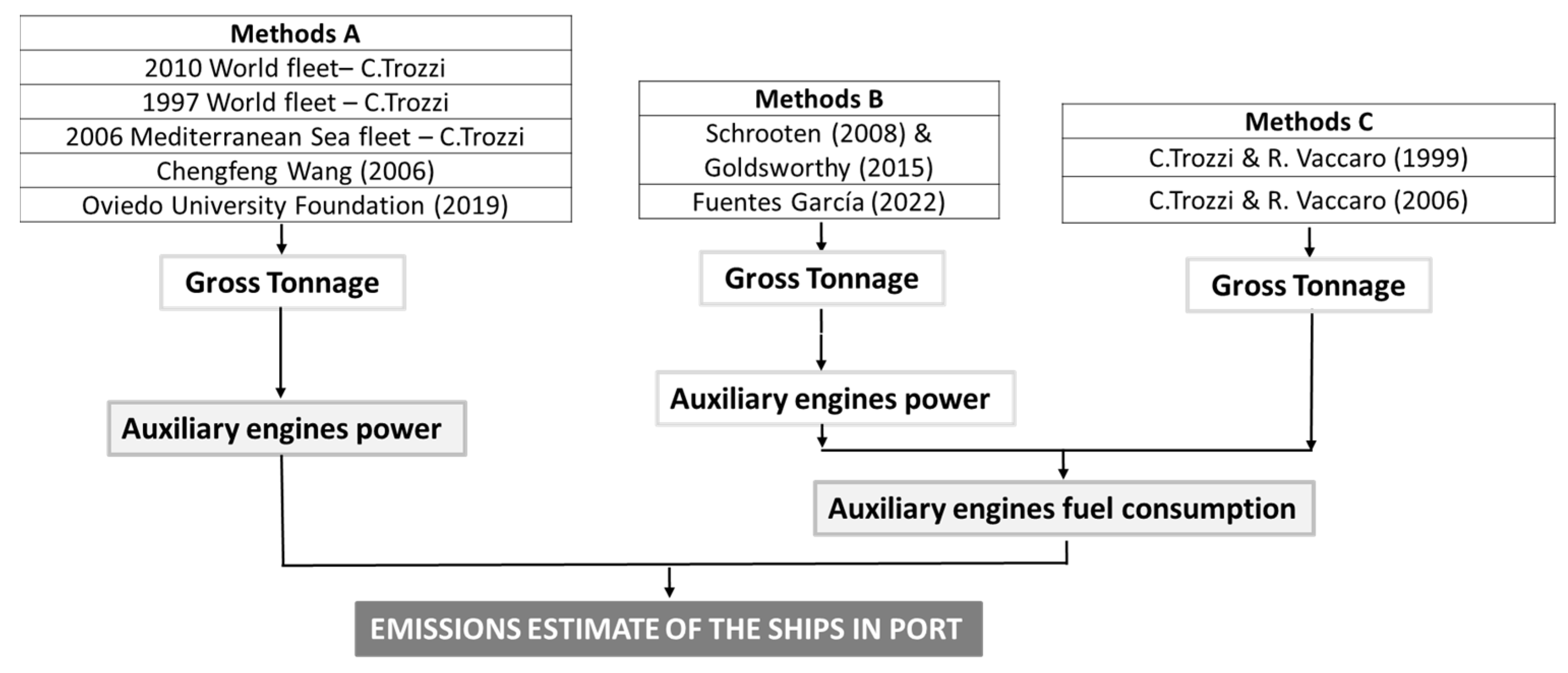
According to Figure 1, the methods analyzed in this article can be classified into three groups:

• Methods A: Calculate emissions from the estimated power of the auxiliary engines;
• Methods B: Obtain emissions through the fuel consumption estimated from the power of the auxiliary engines;
• Methods C: Calculate emissions from estimated fuel consumption directly through the GT.

2.1. Emissions Estimate from Ship’s Auxiliary Engines Power

Generally, the calculation for commercial ships is done on the basis of the emissions for each voyage in the different phase of trip: cruise, maneuvering and hoteling.

$$E_{Trip}=E_{Cruising}+E_{Maneuvering}+E_{Hoteling}$$

(1)

This article only considers the third term in Equation (1), as the estimation will be made based on the following aspects:

• During their stay in port, the ships use their auxiliary engines (AE) to produce electricity in loading, unloading and hoteling operations [2,3,4];
• Because Vigo is a European port, engines can only use marine fuel with a limit of 0.1% sulfur content by mass such as marine gas oil (MGO) of 0.1% [12];
• The type of diesel engine for Ro–Ro ships will be considered as medium-speed [4,37].

During the ships’ stay in port, the emissions estimation method for their AEs and each pollutant takes into account the time the AEs operate for each type of ship, their power, time hoteling, load factor and emissions factor for each pollutant being considered [5,26,37,38,39].

$$E_{Hoteling,i}=\frac{T_h·P_{AE}·L{F}_{AE}·E{F}_i}{{10}^3}$$

(2)

where:

• E_Hoteling,i: emission for hoteling (t) of “i” pollutant;
• i: pollutant (NO_x, SO₂, CO₂, VOC, PM, CO, N₂O);
• T_h: time for hoteling (h);
• P_AE: auxiliary engine nominal power (kW);
• LF_AE: auxiliary engine load factor (

  Table 2. Calculation methods for the auxiliary engine power for hoteling of Ro–Ro ships as a function of GT.

  Method	PME (kW)		Ratio AE/ME	LFAE
  2010 World fleet	164.578·GT0.4350	(3)	0.24	0.4
  1997 World fleet	35.93·GT0.5885	(4)	N/A	0.4
  2006 Mediterranean Sea fleet	45.7·GT0.5237	(5)	0.39	0.4
  Wang	692.09·GRT0.2863	(6)	N/A	N/A
  Oviedo UF	206.1793·GT0.3967	(7)	N/A	0.4

  );
• EF_i: emission factor of “i” pollutant (kg/kW).

Other sources also consider other factors for adjustment:

• When the engines work at low load [40], in order to obtain the increase in emissions for this situation, in the case of auxiliary engines, this factor is considered to be 1, which means it does not affect the estimate;
• In order to reflect environmental benefits obtained by installing emission reduction technologies in the ship and/or engines [8,41], this factor will not be applied in this article.
• Therefore, regarding the parameters defined in Equation (2), it can be seen that:
• The emission factors were taken from the reports by ENTEC 2010 [37] (

  Table 3. AE emission factors (g/kWh) for hoteling ENTEC 2010 [37].

  Engine/Fuel Type	NOx Pre-2000 Engine	NOx Post-2000 Engine	NOx Fleet Average	SO2	CO2	VOC	PM10 PM2.5	SFC *
  Medium–high-speed/MGO	13.9	11.5	13.0	0.9	690	0.4	0.3	217

  * SFC: Specific fuel consumption.

  ), USA EPA 2009 [4] (

  Table 4. AE emission factors (g/kWh) for hoteling USA EPA 2009 [4].

  Fuel Type	NOx	PM10	PM2.5	SOx	CO2	VOC	CO	SFC
  0.1% MGO	13.9	0.18	0.17	0.42	690.71	0.4	1.1	217

  ) and Port of Los Angeles 2020 [42] (

  Table 5. AE emission factors (g/kWh) for hoteling, Port of Los Angeles 2020 [42].

  Engine/Fuel Type	Tier	NOx	PM10	PM2.5	SOx	CO2	VOC	CO	N2O	CH4
  Medium-speed/0.1% MGO	1	12.2	0.19	0.17	0.42	696	0.4	1.1	0.029	0.008
  	2	10.5
  High-speed/0.1% MGO	1	9.8						0.9
  	2	7.7

  );
• The number of hours the ships are in port (T_h) was obtained from the analysis of Ro–Ro ships in the Port of Vigo (Section 3.1);
• No information was available on either the auxiliary engines’ power or their load factors.

Regarding this final point, various methods were encountered in the bibliographical review on the methodology for estimating ship emissions (Table 2), which obtain the main engines power (P_ME) according to GT by means of non-linear regression curves.

All the methods use GT, except Wang [27], who used gross registered tonnage (GRT). The equivalence between GRT and GT is 1 GT = 1.875 GRT [5]. GRT was substituted by GT when the IMO adopted the International Convention on Tonnage Measurement of Ships on 23 June 1969.

Moreover, auxiliary engine power for hoteling is obtained according to main engine power, the estimated average vessel ratio of auxiliary engines/main engines (AE/ME), and the % load of MCR (maximum continuous rating) of auxiliary engines for hoteling (LF_AE).

2.2. Emissions Estimate from Auxiliary Engines Fuel Consumption

The emissions for each pollutant obtained from auxiliary engines’ fuel consumptions and the emission factors for each pollutant for hoteling are shown in

Table 6. Tier 1 engine emission factors (kg/t) for hoteling [38,43].

Fuel Type	NOx	CO	NMVOC *	SOx	PM10	PM2.5
MDO-MGO	78.5	7.4	2.8	20	1.5	1.4

* NMVOC: Non-methane volatile organic compounds.

and

Table 7. Tier 2 engine emission factors (kg/t) for hoteling [38,43].

Engine/Fuel Type	NOx 2000	NOx 2005	NOx 2010	CO	NMVOC	SOx	PM10	PM2.5
Medium-speed/MDO-MGO	65.0	63.1	60.6	7.4	2.8	20	1.5	1.3
High-speed/MDO-MGO	59.1	57.1	55.1

. [5,38,43].

$$E_{Hoteling,i }=\frac{T_h·FC·E{F}_i}{{10}^3}$$

(8)

where:

• E_Hoteling,i: emission for hoteling (t) of “i” pollutant;
• T_h: time for hoteling (h);
• FC: fuel consumption (t_fuel/h);
• EF_i: emission factor of “i” pollutant (kg/t_fuel).

Emission factors for auxiliary engines and marine gas oil (MGO) were taken from Trozzi [38,43]. However, marine diesel oil (MDO) is also inclued in the fuel type. Even though emissions factors for further pollutants may exist, the analysis focuses on those that are similar to those obtained from auxiliary engine power, and that have the most relevant effects, as mentioned in the introduction (Table 6).

In this case, data for fuel consumption do not exist either, but they can be estimated theoretically by means of different methods according to GT or auxiliary engines power (

Table 8. Calculation methods for fuel consumption (FC) of Ro–Ro ships as a function of GT or P_AE.

Method	FC (tfuel/h)
Method 1999—Trozzi and Vaccaro	$\frac{\left(12.834+0.00156·\mathrm{GT}\right)·p_m}{24}$	(9)
Method 2006—Trozzi and Vaccaro	$\frac{\left(6.3501+0.0013·\mathrm{GT}+1.6852{\mathrm{E}}^{-7}{\mathrm{GT}}^2-6.2691{\mathrm{E}}^{-12}·{\mathrm{GT}}^3+5.699{\mathrm{E}}^{-17}·{\mathrm{GT}}^4\right)·p_m}{24 }$	(10)
Schrooten and Goldsworthy	$\frac{SFC·L{F}_{AE}·P_{AE}}{{10}^6}$	(11)
Fuentes García	$\frac{HV·L{F}_{AE}·P_{AE}}{{10}^3}$	(12)

).

where:

• p_m: The fraction of maximum fuel consumption for different operation modes, taking into account a 0.2 value for hoteling default [28,29,30,31,32,33,34];
• SFC: Specific fuel consumption (g/kWh). Taking into account a medium- or high-speed diesel engine that uses marine gas oil as fuel, its hoteling-specific consumption would be 217 (g/kWh) for auxiliary engines [38].
• LF_AE: Percentage load of MCR (maximum continuous rating) of auxiliary engine for hoteling (Table 2) [5,38].
• HV: Heating value of fuel consumption (MJ/kg fuel). Considering marine gas oil as fuel, its value is 42.65 MJ/kg fuel [37] or 1 kg fuel/11.847 kWh.

Trozzi and Vaccaro (Equations (9) and (10)) established two calculation methods based on GT. In addition to Ro–Ro ships, they also include passenger and cargo vessels, which means that they are not as specific as calculating power from GT.

In the two final methods (Equations (11) and (12)), the auxiliary engine power is obtained from an estimation of the main engine power and an estimated average vessel ratio of auxiliary engines/main engines (AE/ME) by ship type, as described in the previous section.

2.3. Advantages and Disadvantages of Methods

Initially, all methods need to take into account GT to calculate emissions.

According to Table 2, only two calculation methods for the auxiliary engine power have all necessary values to obtain emissions (2010 World fleet and 2006 Mediterranean Sea fleet [5]). The AE/ME ratio or LF_AE is not available for the other three methods.

This problem would also affect the two methods used to calculate emissions from auxiliary engines’ fuel consumption (Schrooten [26] and Goldsworthy [44], and Fuentes García [32]), because they need to obtain the auxiliary engines’ power, and the 2010 World fleet method is applied to both cases.

Nevertheless, the methods that calculate emissions from the estimated fuel consumption directly through the GT have no problem.

In reference to engine emission factors for hoteling:

• Emissions estimation methods from auxiliary engines’ fuel consumption include both marine diesel oil and marine gas oil. Marine diesel oil usually has a higher percentage of sulfur content than marine gas oil and therefore is more pollutant. Additionally, the CO₂ emission factor is not available for these methods;
• Emissions estimation methods from auxiliary engines’ power use an emission factor adjusted to the fuel type “0.1% MGO” and comply with the limit of 0.1% sulfur content established by Directive (UE) 2016/802.

3. Application to Ro–Ro Ships in the Port of Vigo

Below, the various methods described in the previous section and in Figure 1 are applied to the specific case of Ro–Ro ships that have stopped in the Port of Vigo. The ultimate aim is to compare the methods and determine the most ideal calculation methodology.

3.1. Initial Data: Port Location and Ships under Study

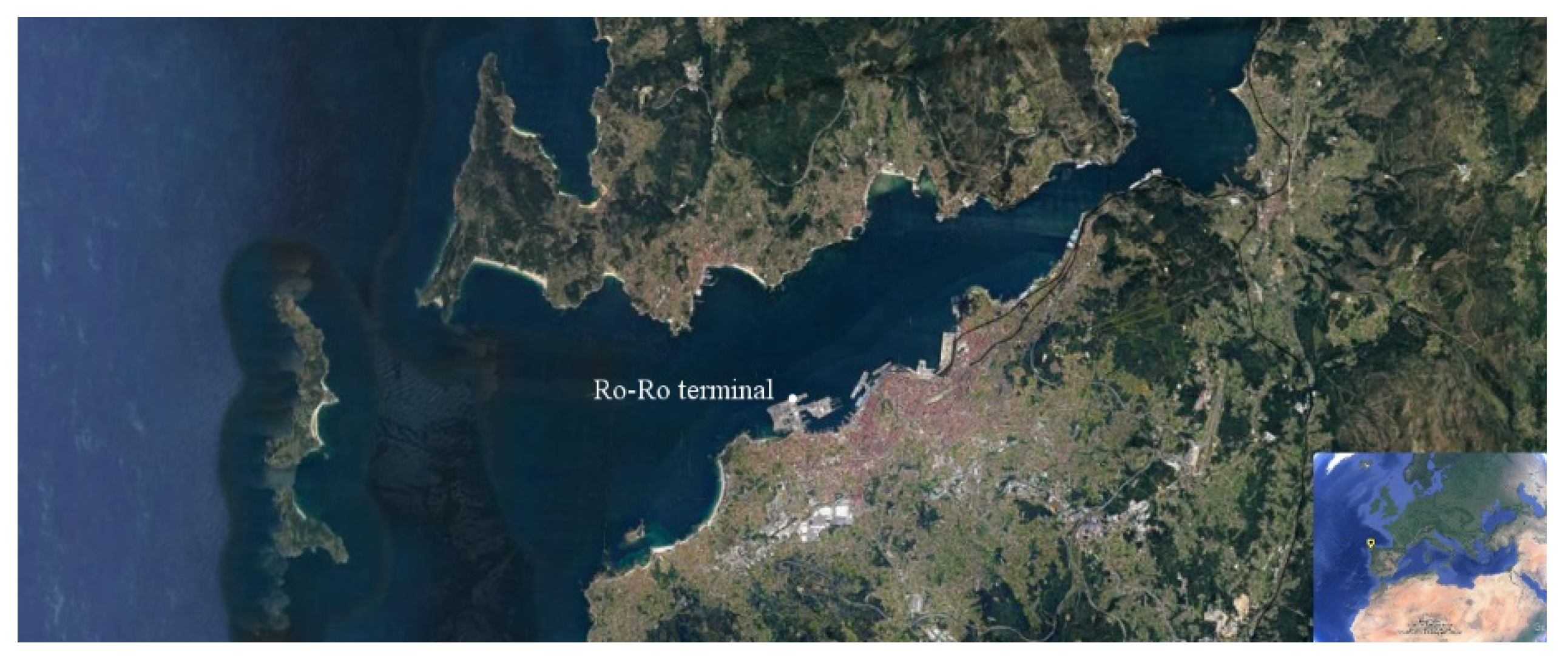
The Port of Vigo is located in the northwest of Spain, as shown in Figure 2. Being a port on the Atlantic Ocean makes it relevant for maritime routes. As far as goods shipping is concerned, the Ro–Ro lines stand out both at the European and transoceanic levels [23], as an important automotive company is also located in the city of Vigo. Moreover, the time Ro–Ro ships stayed in port was 9757 h for Vigo in 2018, compared to 606.5 h for transatlantic traffic—some 16 time higher [24,25]. For this reason, this study focused on Ro–Ro ship traffic in the Port of Vigo.

The initial basis for this work is a Report of the Port Authority of Vigo (PAV), which included a viability study for the implementation of an onshore power supply (OPS) system, for application with the Ro–Ro ships that berth at the Port of Vigo [24]. The criteria followed in this report for the inclusion of ships were as follows (

Table A2. Ro–Ro ships selected in the PAV Report [24].

Ship	Length (m)	GT	Annual Berths	Hours per Year	Average Time Spent in Berthing (h)
SUAR VIGO	140	16,361	79	1601	20.27
BOUZAS	149	15,224	76	2066	27.19
GALICIA	149	16,361	31	868	28.01
TENERIFE CAR	133	13,112	28	306	10.91
ARABIAN BREEZE	164	29,874	23	411	17.86
RCC PASSION	168	36,834	21	434	20.66
VERONA	177	37,237	18	263	14.63
BALTIC BREEZE	164	29,979	17	337	19.84
CORAL LEADER	176	40,986	12	200	16.64
EMERALD LEADER	176	40,986	12	167	13.95
NEPTUNE KELAFONIA	170	36,825	12	105	8.72
NEPTUNE GALENE	170	37,602	11	108	9.85
OPAL LEADER	176	40,986	11	172	15.64
VEGA LEADER	180	51,496	11	171	15.55
VICTORY LEADER	186	49,675	11	168	15.31

):

• Minimum number of berthings per year: 10 (regular lines);
• Minimum total stay time per year: 100 h;
• Minimum stay time: 8.5 h (for the connection to be operational).

To determine the methodology for calculating emissions, it was deemed ideal to define them for ships that berth in Vigo with some regularity and that have a relevant level of activity. For that reason, these criteria were adopted for the selection of ships.

Because the data on berths from the PAV are from 2018, it was decided to update them by tracking Ro–Ro ships stopping in Vigo between July 2021 and March 2022, by means of open access information available from the MarineTraffic [45], VesselFinder [46] and vesseltracker.com [35] websites.

This tracking detected three vessels that were out of service (Verona, Baltic Breeze and Arabian Breeze) and led to the addition of four more (Viking Amber, Viking Diamond, Mosel Ace and Prometheus Leader), which had berthed regularly during the tracking period and whose annual data could be estimated.

Starting from these considerations, the ships given in

Table 9. Ro–Ro ships selected and initial data.

Ship	Length (m)	GT	Year Built	Flag	No. of Annual Berths (Berths/Year)	Hours per Year (h/Year)	Average Time Spent in Berthing (h)
Suar Vigo	140	16,361	2003	Spain	79	1601	20
Bouzas	149	15,224	2002	Spain	76	2066	27
Galicia	149	16,361	2003	Portugal	31	868	28
Tenerife Car	133	13,112	2002	Portugal	28	306	11
RCC Passion	168	36,834	2011	Bahamas	21	434	21
Coral Leader	176	40,986	2006	Bahamas	12	200	17
Emerald Leader	176	40,986	2008	Bahamas	12	167	14
Neptune Kefalonia	170	36,825	2009	Malta	12	105	9
Neptune Galene	170	37,602	2014	Greece	11	108	10
Opal Leader	176	40,986	2007	Bahamas	11	172	16
Vega Leader	180	51,496	2000	Panama	11	171	16
Victory Leader	186	49,675	2010	Bahamas	11	168	15
Viking Amber	167	39,362	2010	Singapore	28	474	17
Viking Diamond	167	39,362	2011	Singapore	33	283	9
Mosel Ace	176	37,237	2000	Liberia	24	244	10
Prometheus Leader	190	41,886	2008	Singapore	10	199	20

were selected. The table gives the corresponding characteristics that were used to establish the emissions estimation methodology.

It shows that the interval for GT for the selected ships was approximately between 13,000 and 52,000 and for the annual hours spent berthing, between 105 and 2066 h.

3.2. Auxiliary Engines Power Estimate of Ro–Ro Ships

From the GT data for each ship given in Table 9 and the methods described in Table 2, the auxiliary engines’ nominal power was obtained (

Table 10. Auxiliary engines’ consumed power (kW) estimate considering load factor of 0.4.

Ship	2010 World Fleet (3)	1997 World Fleet (4)	2006 Mediterranean Sea Fleet (5)	Wang (6)	Oviedo UF (7)	5 Methods Average	2010/2006 Average
Suar Vigo	1075.60	1041.25	1147.66	892.66	929.25	1017.29	1111.63
Bouzas	1042.42	998.04	1105.18	874.44	903.08	984.63	1073.80
Viking Diamond	1575.80	1745.55	1817.53	1147.74	1316.39	1520.60	1696.67
Galicia	1075.60	1041.25	1147.66	892.66	929.25	1017.29	1111.63
Tenerife Car	976.85	914.06	1022.03	837.84	851.13	920.38	999.44
Viking Amber	1575.80	1745.55	1817.53	1147.74	1316.39	1520.60	1696.67
Mosel Ace	1538.21	1689.46	1765.47	1129.65	1287.72	1482.10	1651.84
RCC Passion	1530.95	1678.67	1755.44	1126.14	1282.17	1474.67	1643.19
Coral Leader	1603.76	1787.58	1856.43	1161.10	1337.67	1549.31	1730.09
Emerald Leader	1603.76	1787.58	1856.43	1161.10	1337.67	1549.31	1730.09
Neptune Kefalonia	1530.79	1678.43	1755.21	1126.06	1282.05	1474.51	1643.00
Neptune Galene	1544.76	1699.18	1774.51	1132.81	1292.71	1488.79	1659.63
Opal Leader	1603.76	1787.58	1856.43	1161.10	1337.67	1549.31	1730.09
Vega Leader	1771.19	2044.59	2092.17	1239.52	1464.46	1722.39	1931.68
Victory Leader	1743.66	2001.73	2053.09	1226.81	1443.69	1693.80	1898.38
Prometheus Leader	1618.99	1810.57	1877.67	1168.35	1349.25	1564.96	1748.33

), taking the following aspects into account:

• As the 1997 World fleet [5], Wang [27] and Oviedo UF [36] methods do not have an average ratio for auxiliary engines/main engines (AE/ME), the value of 0.24 (Table 2) was considered, which corresponds to 2010 World fleet [5].
• For the Wang [27] method, a load factor (LF_AE) of 0.4 was also considered, as it is not specified in the method (Table 2).

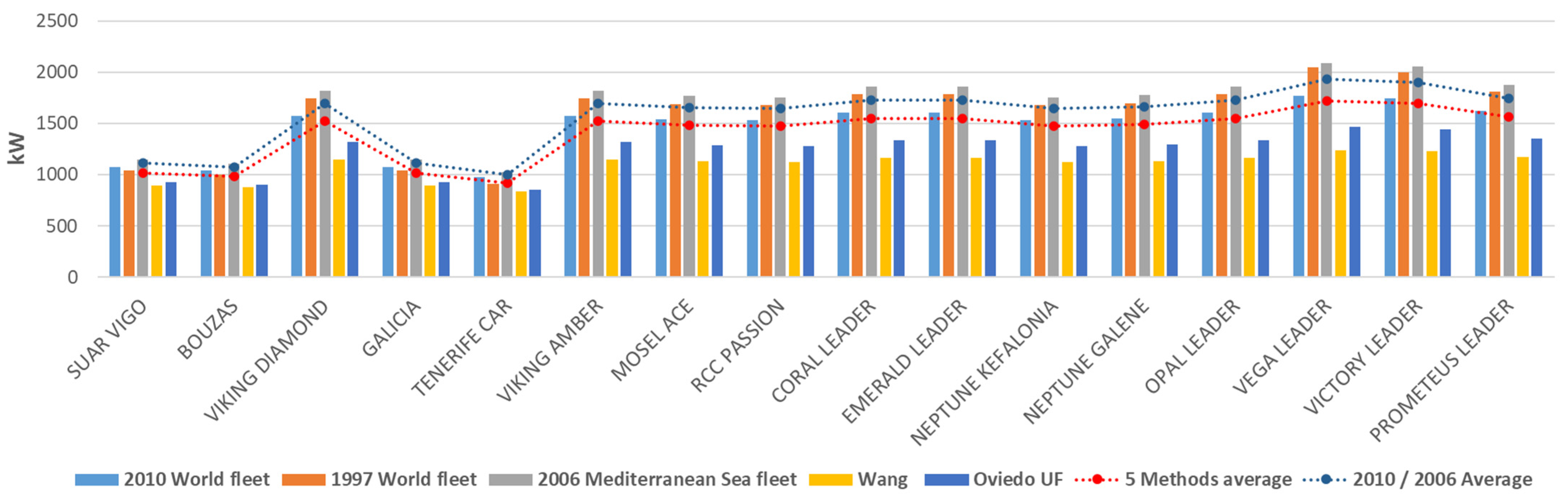
Therefore, only the 2010 World fleet and 2006 Mediterranean Sea fleet methods have all the data needed to undertake the estimation of auxiliary engine power from the GT, as the AE/ME ratio and load factor (LF) are known (Table 2). That is why it is considered important to include the average value of the five methods, and the average value of 2010 World fleet–2006 Mediterranean Sea fleet as a reference range for errors when comparing the results and a criteria for selecting the estimation method to be used in this article (Table 10 and Figure 3).

When considering the AE/ME ratio of 0.24 in the methods where these data were not available, the average obtained between 2010 World fleet and 2006 Mediterranean Sea fleet was 11% higher than the five methods’ average.

Therefore, the procedure with results most in line with the established reference range was selected.

From the results obtained, it was considered better to take into account the auxiliary engines’ nominal power calculated through the 2010 World fleet method for the following reasons:

• Only in the 2010 World fleet and 2006 Mediterranean Sea fleet methods are all calculation data specified;
• The 2010 World fleet method covers a larger geographical area than the 2006 Mediterranean Sea fleet and is more in line with the location of the Port of Vigo as it is situated in the Atlantic Ocean;
• Auxiliary engines’ power calculated with the 2010 World fleet method is usually within the reference range, while the 2006 Mediterranean Sea fleet figure is usually higher (Figure 3).

3.3. Auxiliary Engines Fuel Consumption Estimate of Ro–Ro Ships

As already mentioned in the methodology section, there are two ways of estimating fuel consumption, either directly from GT or from auxiliary engines’ power, also obtained from GT.

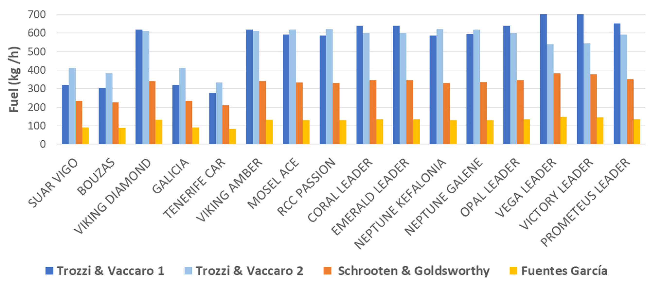
In the results shown in

Table 11. Fuel consumption (kg/h) estimate comparison in port.

Ship	Method 1999—C. Trozzi and R. Vaccaro (9)	Method 2006—C. Trozzi and R. Vaccaro (10)	Schrooten and Goldsworthy (11)	Fuentes García (12)
Suar Vigo	319.64	411.31	233.40	90.79
Bouzas	304.86	384.50	226.21	87.99
Viking Diamond	618.66	609.15	341.95	133.01
Galicia	319.64	411.31	233.40	90.79
Tenerife Car	277.41	332.67	211.98	82.45
Viking Amber	618.66	609.15	341.95	133.01
Mosel Ace	591.03	619.24	333.79	129.84
RCC Passion	585.79	620.70	332.22	129.22
Coral Leader	639.77	599.26	348.02	135.37
Emerald Leader	639.77	599.26	348.02	135.37
Neptune Kefalonia	585.68	620.73	332.18	129.21
Neptune Galene	595.78	617.78	335.21	130.39
Opal Leader	639.77	599.26	348.02	135.37
Vega Leader	776.40	540.40	384.35	149.50
Victory Leader	752.73	544.41	378.38	147.18
Prometheus Leader	651.47	593.20	351.32	136.66
Total	8917.04	8712.32	5080.38	1542.81

and Figure 4, a difference of only 10% can be observed between the Trozzi and Vaccaro methods [28,29,30,31,32,33,34], probably due to the former being adjusted by means of linear regression, and the latter by a fourth-degree polynomial regression. However, there is a notable difference among the methods that calculate consumption from auxiliary engine power. The Schrooten [26] and Goldsworthy [44] methods take specific fuel consumption into account, and the Fuentes García method [32] considers the fuel heating value, representing only 30% of the consumption obtained by Schrooten [26] and Goldsworthy [44].

Specific fuel consumption compares the ratio of fuel used by an engine to produce a given amount of power. It allows engines to be compared, regardless of size, to establish which is the most efficient, i.e., the one that will use the least amount of fuel to produce the most power. However, the heating value is the amount of energy per unit of mass or unit of volume that can be released when an oxidation chemical reaction takes place. Therefore, the engine performance would also need to be known for them to be equivalent.

Consequently, they are considered to be different concepts, and in relation to a ship’s engine, specific fuel consumption would be more appropriate, as it also depends on the type and characteristics of the engine itself: slow-, medium- and high-speed diesel engines, gas turbine, or steam turbine.

Consequently, if the Trozzi and Vaccaro methods, which are calculated from GT, are compared with those of Schrooten and Goldsworthy, which are based on auxiliary engines’ power, it can be seen that the former give total fuel consumptions around 40% higher. This circumstance may be due to the fact that Trozzi and Vaccaro calculate the fuel consumption as follows:

• On the basis of a general parameter for the ship, such as GT;
• Without differentiating whether it corresponds to a main or auxiliary engine and speed (slow, medium or high);
• Without taking fuel type into account, as the calculation not only uses the power but also the specific consumption for marine gas oil (MGO), which is lower than that for fuel oil;
• For a set of ships including Ro–Ro, passenger and cargo, which are different in the way they are constructed and operated. The calculation is not exclusive for Ro–Ro as in the case of the calculation from power.

Thus, the Schrooten and Goldsworthy methods are considered as a better option to characterize fuel consumption, and subsequently emissions, as they consider more detailed technical information and differentiate the following:

• Whether they correspond to medium- and high-speed auxiliary engines;
• Fuel type used (MGO);
• Calculations that are specific to Ro–Ro ships.

Consequently, they also start with the engine power calculated from GT, applying regression equations.

3.4. Auxiliary Engines’ Emissions Estimate

Emissions calculations were made from both the auxiliary engines’ power of ships and their fuel consumption, in order to compare the results from the two methods and select the calculation methodology for this article.

Emissions estimation from engines’ power was calculated using Equation (2) for each of the pollutants (

Table 12. Emissions (t/year) calculation from power with 0.1% MGO.

Ship	NOx	PM10	PM2.5	SOx	CO2	VOC	CO	N2O	CH4	Total per Ship
Suar Vigo	21.01	0.33	0.29	0.72	1198.54	0.69	1.89	0.050	0.014	1223.53
Bouzas	26.27	0.41	0.37	0.90	1498.93	0.86	2.37	0.062	0.017	1530.20
Viking Diamond	5.44	0.08	0.08	0.19	310.60	0.18	0.49	0.013	0.004	317.08
Galicia	11.39	0.18	0.16	0.39	649.80	0.37	1.03	0.027	0.007	663.35
Tenerife Car	3.14	0.06	0.05	0.13	208.05	0.12	0.33	0.009	0.002	211.88
Viking Amber	9.12	0.14	0.13	0.31	520.29	0.30	0.82	0.022	0.006	531.15
Mosel Ace	4.57	0.07	0.06	0.16	260.80	0.15	0.41	0.011	0.003	266.24
RCC Passion	8.11	0.13	0.11	0.28	462.45	0.27	0.73	0.019	0.005	472.09
Coral Leader	3.91	0.06	0.05	0.13	223.24	0.13	0.35	0.009	0.003	227.90
Emerald Leader	3.27	0.05	0.05	0.11	186.41	0.11	0.29	0.008	0.002	190.30
Neptune Kefalonia	1.96	0.03	0.03	0.07	111.87	0.06	0.18	0.005	0.001	114.20
Neptune Galene	1.75	0.03	0.03	0.07	116.12	0.07	0.18	0.005	0.001	118.25
Opal Leader	3.37	0.05	0.05	0.12	191.99	0.11	0.30	0.008	0.002	195.99
Vega Leader	3.70	0.06	0.05	0.13	210.80	0.12	0.33	0.009	0.002	215.20
Victory Leader	3.08	0.06	0.05	0.12	203.88	0.12	0.32	0.008	0.002	207.64
Prometheus Leader	3.38	0.06	0.05	0.14	223.89	0.13	0.35	0.009	0.003	228.01
Total	113.46	1.80	1.61	3.97	6577.66	3.78	10.40	0.274	0.076	6713.01

) The emission factors from the Port of Los Angeles 2020 [42] were considered as it is the most recent and complete study in terms of fuel type, engine type (Tier 1 and 2) and polluting components. Furthermore, the engine speed was set at medium as in the cases of the PVA Report [24] and the USA EPA 2009 [4].

Of all the pollutants analyzed, the carbon dioxide emissions represent 98% of the total of 6.7 t/year. All the other pollutants only represent 2%, although they are relevant because of their damaging effects to human health.

Regarding the emissions estimation from fuel consumption (

Table 13. Emissions (t/year) estimation from MDO/MGO fuel consumption.

Ship	Consumption (t/Year)	NOx	SOx	CO	NMVOC	PM10	PM2.5	Total per Ship
Suar Vigo	373.68	29.33	7.47	2.77	1.05	0.56	0.49	41.67
Bouzas	467.34	36.69	9.35	3.46	1.31	0.70	0.61	52.11
Viking Diamond	96.84	7.60	1.94	0.72	0.27	0.15	0.13	10.80
Galicia	202.60	15.90	4.05	1.50	0.57	0.30	0.26	22.59
Tenerife Car	64.86	3.93	1.30	0.48	0.18	0.10	0.08	6.07
Viking Amber	162.22	12.73	3.24	1.20	0.45	0.24	0.21	18.09
Mosel Ace	81.31	6.38	1.63	0.60	0.23	0.12	0.11	9.07
RCC Passion	144.18	11.32	2.88	1.07	0.40	0.22	0.19	16.08
Coral Leader	69.60	5.46	1.39	0.52	0.19	0.10	0.09	7.76
Emerald Leader	58.12	4.56	1.16	0.43	0.16	0.09	0.08	6.48
Neptune Kefalonia	34.88	2.74	0.70	0.26	0.10	0.05	0.05	3.89
Neptune Galene	36.20	2.19	0.72	0.27	0.10	0.05	0.05	3.39
Opal Leader	59.86	4.70	1.20	0.44	0.17	0.09	0.08	6.67
Vega Leader	65.72	5.16	1.31	0.49	0.18	0.10	0.09	7.33
Victory Leader	63.57	3.85	1.27	0.47	0.18	0.10	0.08	5.95
Prometheus Leader	69.81	4.23	1.40	0.52	0.20	0.10	0.09	6.53
Total	2050.79	156.79	41.02	15.18	5.74	3.08	2.67	224.47

) the following were taken into account:

• The emission factors in Table 6 and Table 7 considering medium-speed and differentiating between Tier 1 and 2;
• The fuel consumption obtained using the Schrooten [26] and Goldsworthy [44] methods in Table 11

In this case, the total emissions are much lower because the carbon dioxide emission factor is not available. However the emissions calculated from fuel consumption for all other pollutants (NO_x, SO_x, CO, VOC, PM₁₀, PM_2.5) are greater than the values obtained from those methods using engine power (

Table 14. Emissions (t/year) comparison calculation.

Calculation	NOx	PM10	PM2.5	SOx	CO2	VOC	CO	N2O	CH4
From consumption fuel	156.79	3.08	2.67	41.02	N/A	5.74	15.18	N/A	N/A
From power engine	113.46	1.80	1.61	3.97	6577.66	3.78	10.40	0.274	0.076
From consumption fuel/From power engine	1.38	1.71	1.66	10.33	N/A	1.52	1.46	N/A	N/A

).

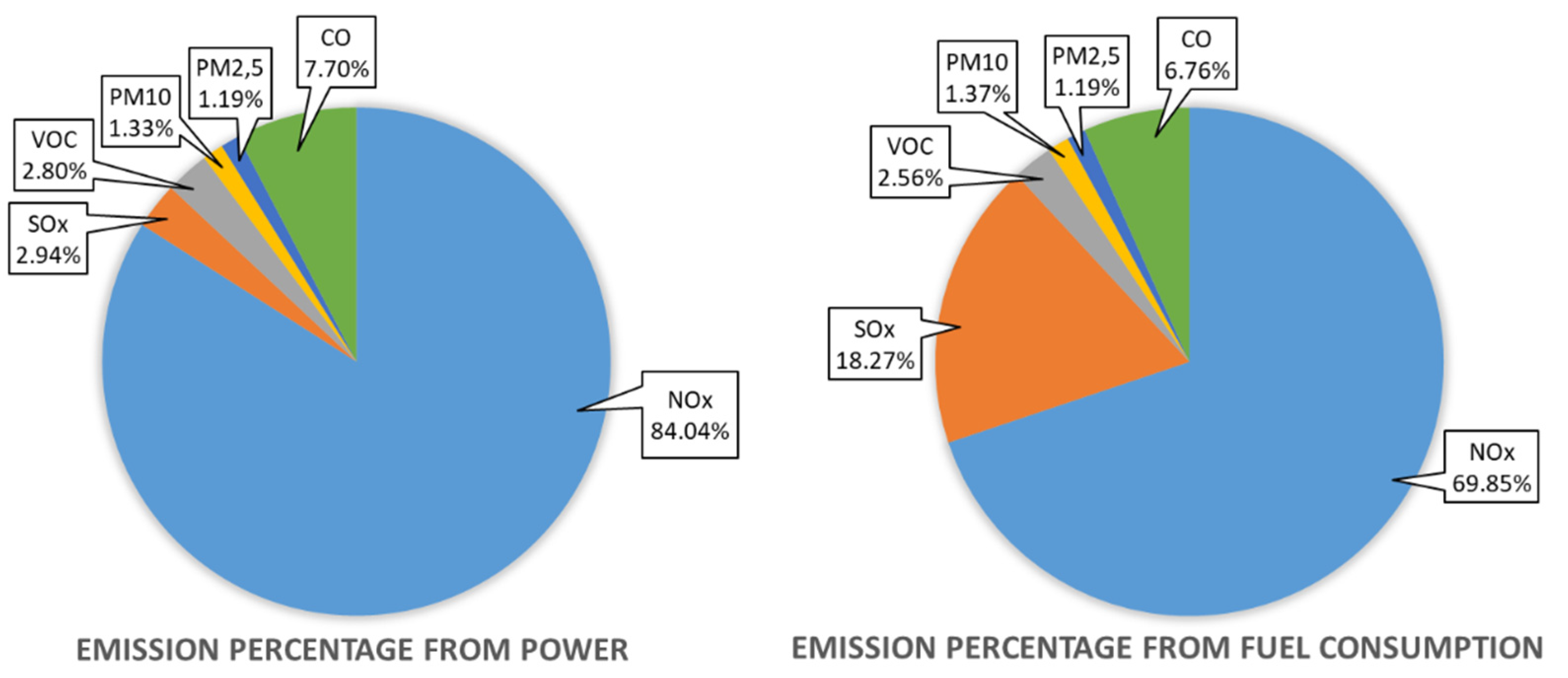
If the comparison is made with respect to the emission percentages (Figure 5), the greatest variation is produced in the NO_x and SO_x pollutants. The percentage of NO_x is greater with the estimation based on power, while the percentage of SO_x is greater when it is based on fuel consumption. The percentages for the rest of the pollutants are similar.

3.5. Emissions Estimation Method Selection

Based on the analysis carried out, it was considered a better option to obtain emissions from the auxiliary engines’ power of ships than from consumption, for the following reasons:

• The fuel consumption of ships is not known. According to Trozzi [5,43], emissions’ calculations using fuel consumption tend to be used when detailed infomation is available on the consumption for each type of ship and engine. Otherwise, it is better to calculate using power;
• Auxiliary engines’ power includes a carbon dioxide emission factor (CO₂), in addition to PM, VOCs, CO, NO_x and SO_x [8]. Consequently, they should be analyzed together;
• The emission factors already take into account the 0.1% MGO demanded by European ports and the tier of each type of ship and are specific for medium-speed. The calculation using fuel consumption, however, does not specify the MGO percentage, which could probably exceed what is demanded, as it is included with the marine diesel oil (MDO).

Consequently, the emissions estimation for each pollutant produced for the auxiliary engines of the Ro–Ro ships during their stay in port was carried out using Equation (13), considering:

• Only times when the ship is berthing in port;
• A ratio of auxiliary engines/main engines (AE/ME) of 0.24;
• The load factor (LF_AE) of 0.4 corresponding to their stay in port (hoteling).

$$\begin{gathered} E_{Hoteling,i}=\frac{T_h·P_{AE}·L{F}_{AE}·E{F}_i}{{10}^3}=\frac{T_h·\left(164.578·G{T}^{0.4350}·0.24\right)·0.4·E{F}_i}{{10}^3} \\ {E}_{Hotelling,i}=\frac{15.7995·T_h·G{T}^{0.4350}·E{F}_i}{{10}^3} \end{gathered}$$

(13)

where:

• E_hoteling,i: total emissions of pollutants for hoteling (t) of “i” pollutant;
• EF_i: emission factor of “i” pollutant (kg/kW);
• GT: gross tonnage of the ship;
• T_h: time for hoteling (h);
• i: pollutant (CO₂, PM, VOCs, CO, NO_x and SO_x).

Thus, the total emissions’ estimation in the Port of Vigo of the Ro–Ro ships analyzed, with respect to the pollutants under consideration, amounts to some 6.7 kt, according to Table 12.

4. Simplified Method Proposal

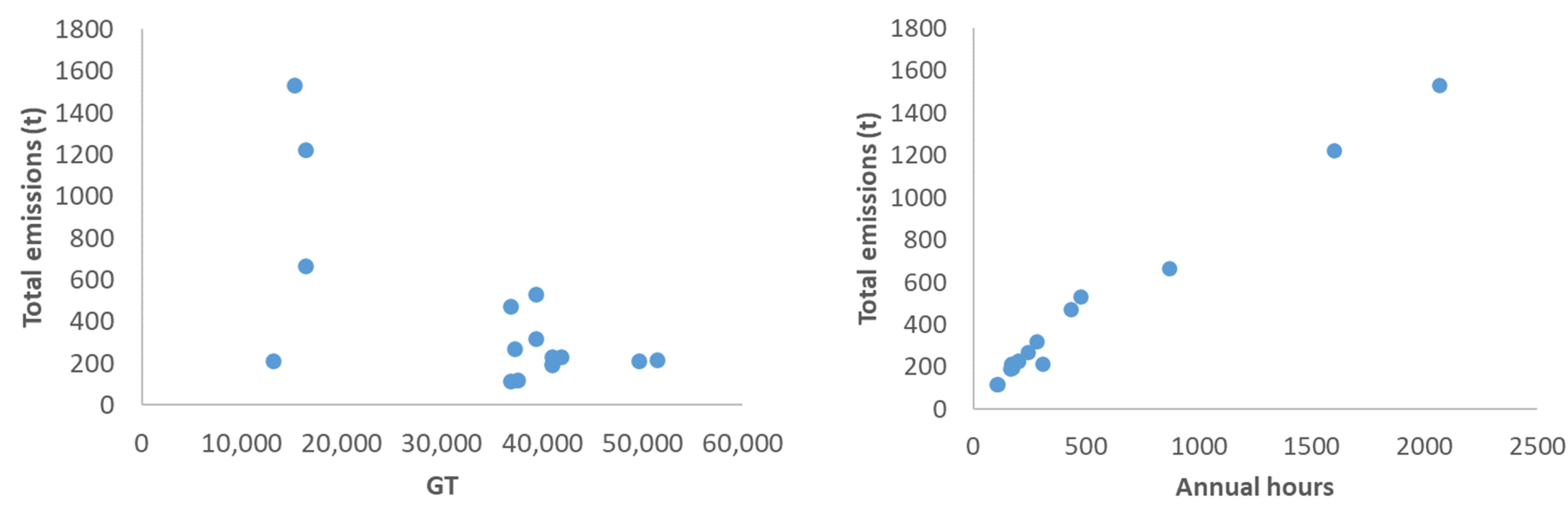
In this section, a simplified method for calculating emissions will be introduced. As a starting point, an analysis is made of Equation (13), where it can be observed that the emissions vary according to the time for hoteling (T_h) and GT, for each pollutant emission factor. Initially, it can be seen that the emissions increase as the hours spent in berthing increase; but this is not the case for GT (Figure 6).

Adjusting these two parameters by means of a multiple regression, it turns out that in the total emissions calculation the weight of the hours spent in berthing is greater than that of GT (

Table 15. Regression curves in the total emissions calculation.

Regression Type	Equation		R2
Multiple	$E_{total }=-55.0822+0.0033·GT+0.593·T_h$	(14)	0.9913
Simple linear	$E_{total }=84.622+0.7075·T_h$	(15)	0.9865
Simple linear, second-degree polynomial equation	$E_{total }=-6·{10}^{-5}·T_h{}^2+0.826·T_h+59.488$	(16)	0.9879

). Therefore, the option of performing a simple regression based only on time spent is also considered (T_h).

As can be seen in Table 15, the reliability of the curves obtained is very high. The best value for R² is logically obtained with the multiple regression as it considers both parameters, although with the simple regression there is hardly any difference below 0.5%. If total emissions obtained are compared with those resulting from the regression curves using Equation (13), it can be seen that they coincide with the multiple and simple linear regression curves (

Table 16. Results comparison of the total emissions (t/year) estimation from the 16 ships applying regression.

Ship	GT	Annual Hours (h)	Ship Emissions (13) *	Multiple Regression (14)	Linear Regression (15)	Polynomial Regression (16)
Suar Vigo	16,361.00	1601.00	1222.07	1214.97	1217.33	1228.08
Bouzas	15,224.00	2066.00	1528.37	1564.27	1546.32	1509.86
Viking Diamond	39,362.00	283.20	316.70	290.85	284.99	288.56
Galicia	16,361.00	868.00	662.56	658.40	698.73	731.21
Tenerife Car	13,112.00	306.00	212.13	220.87	301.12	306.59
Viking Amber	39,362.00	474.39	530.51	436.03	420.25	437.79
Mosel Ace	37,237.00	243.60	265.92	253.72	256.97	257.10
RCC Passion	36,834.00	434.00	471.53	396.95	391.68	406.63
Coral Leader	40,986.00	200.00	227.63	233.08	226.12	222.25
Emerald Leader	40,986.00	167.00	190.07	208.02	202.77	195.72
Neptune Kefalonia	36,825.00	105.00	114.07	147.11	158.91	145.52
Neptune Galene	37,602.00	108.00	118.40	151.97	161.03	147.96
Opal Leader	40,986.00	172.00	195.76	211.82	206.31	199.74
Vega Leader	51,496.00	171.00	214.94	246.01	205.60	198.94
Victory Leader	49,675.00	168.00	207.89	237.68	203.48	196.52
Prometheus Leader	41,886.00	198.69	228.29	235.08	225.20	221.20
Total			6706.82	6706.82	6706.82	6693.67

* To simplify ship emissions calculations, an average value for NO_x emissions factors is considered, which depends on the auxiliary engine TIER.

).

Next, the equations corresponding to multiple and linear regression curves were compared, in order to establish which one will be used for a simplified calculation of total emissions. For this purpose, the average value and weighted average value, regarding GT and hours spent in berthing in port, were considered as T_h (

Table 17. Average value and weighted average value of GT and T_h of the 16 vessels.

	GT	Th (h/Year)
Average value	34,643.44	472.87
Weighted average value	24,614.49	335.98

).

According to

Table 18. Results comparison of the total emissions estimation from the 16 ships (N) applying regression according to average value and higher frequency of GT and T_h.

N	Th (h/Annual)	GT	Total Emissions (t/Year)
			Calculation (13)	Multiple Regression (14)	Δ Calculation—Multiple (%)	Linear Regression (15)	Δ Calculation—Linear (%)
16	472.87	34,643.44	6706.82	6692.64	0.2	6706.82	0.0
16	472.87	24,614.49	6706.82	6163.11	8.1	6706.82	0.0
16	335.98	34,643.44	6706.82	5029.58	25.0	5157.21	23.1
16	335.98	24,614.49	6706.82	4500.05	32.9	5157.21	23.1

, the best results were obtained with the average values in both regressions, and in the case of the linear regression it coincides exactly with the one calculated from the engines power. Even so, that obtained from the multiple regression is only 0.2% lower.

Consequently, the method based on the linear regression Equation (15) is proposed as the simplified method for calculating total emissions, taking into account the average value for hours spent in berthing of ships in port (T_h,av) and their number (N).

$$E_{Hoteling}=\left(84.6219+0.7075·T_{h,av}\right)·N$$

(17)

If the calculation were required for pollutant type, the regression curves could be obtained for each of those considered in the study, according to

Table 19. Regression equations’ summary proposed by pollutant to calculate emissions from average value GT (GT_av), average value T_h (T_h,av) and number of ships (N).

Pollutant	Multiple Regression Equation		Linear Regression Equation
NOx	$\left(-0.8810+5.3187·{10}^{-5}·G{T}_{av}+0.0121·T_{h,av}\right)·N$	(18)	$\left(1.354+0.0113·T_{h,av}\right)·N$	(19)
PM10	$\left(-0.0147+8.9035·{10}^{-7}·G{T}_{av}+2.0329·{10}^{-4}·T_{h,av}\right)·N$	(20)	$\left(0.0227+1.8942·{10}^{-4}·T_{h,av}\right)·N$	(21)
PM2.5	$\left(-0.0132+7.9663·{10}^{-7}·G{T}_{av}+1.8189·{10}^{-4}·T_{h,av}\right)·N$	(22)	$\left(0.0203+1.6948·{10}^{-4}·T_{h,av}\right)·N$	(23)
SOx	$\left(-0.0326+1.9681·{10}^{-6}·G{T}_{av}+4.4938·{10}^{-4}·T_{h,av}\right)·N$	(24)	$\left(0.0501+4.1872·{10}^{-4}·T_{h,av}\right)·N$	(25)
CO2	$\left(-54.0214+0.0033·G{T}_{av}+0.7447·T_{h,av}\right)·N$	(26)	$\left(82.9922+0.6939·T_{h,av}\right)·N$	(27)
VOC	$\left(-0.0310+1.8744·{10}^{-6}·G{T}_{av}+4.2798·{10}^{-4}·T_{h,av}\right)·N$	(28)	$\left(0.0477+3.9878·{10}^{-4}·T_{h,av}\right)·N$	(29)
CO	$\left(-0.0854+5.1547·{10}^{-6}·G{T}_{av}+0.0012·T_{h,av}\right)·N$	(30)	$\left(0.1312+0.0011·T_{h,av}\right)·N$	(31)
N2O	$\left(-0.0023+1.3590·{10}^{-7}·G{T}_{av}+3.1028·{10}^{-5}·T_{h,av}\right)·N$	(32)	$\left(0.0035+2.8911·{10}^{-5}·T_{h,av}\right)·N$	(33)
CH4	$\left(-6.2094·{10}^{-4}+3.7488·{10}^{-8}·G{T}_{av}+8.5596·{10}^{-6}{T}_{h,av}\right)·N$	(34)	$\left(9.5393·{10}^{-4}+7.9756·{10}^{-6}{T}_{h,av}\right)·N$	(35)
Total	$\left(-55.0822+0.0033·G{T}_{av}+0.7593·T_{h,av}\right)·N$ (see Equation (14))		$\left(84.6219+0.7075·T_{h,av}\right)·N$ (see Equation (17))
Adjusted R2	0.9913		0.9865

.

As in the total emissions calculation, it is also considered acceptable to perform a simplified analysis by considering the average value for hours spent berthing in port (T_h,av). This decision is justified when comparing the resulting equations, as the value of R² adjusted in the linear regression (0.9865) is slightly lower than the value of the multiple regression (0.9913).

Similar to the case of total emissions, the same comparison is now presented for emissions calculation results by pollutant when applying regression equations.

In the calculation for the 16 ships, the linear regression is again found to be more accurate when comparing the results with the emissions obtained from the engines’ power (

Table 20. Emissions estimation results comparison by pollutant for the 16 ships applying regression equations (Table 19).

Pollutant	Emissions (t/Year)
	Calculation	Multiple Regression	Δ Calculation—Multiple (%)	Linear Regression	Δ Calculation—Linear (%)
NOx	107.27	106.93	0.3	107.16	0.1
PM10	1.80	1.80	0.0	1.80	0.0
PM2,5	1.61	1.61	0.0	1.61	0.0
SOx	3.97	3.97	0.0	3.97	0.0
CO2	6577.66	6599.15	−0.3	6577.84	0.0
VOC	3.78	3.78	0.0	3.78	0.0
CO	10.40	10.57	−1.7	10.42	−0.2
N2O	0.27	0.27	0.3	0.27	−0.2
CH4	0.08	0.08	0.0	0.08	0.0
Total sum	6706.82	6728.15	−0.3	6706.93	0.0
Total per equation	6706.82	6692.64	0.2	6706.82	0.0

).

Furthermore, as all the linear regression equations have the same adjusted R² value, it can be seen that there is a proportionality between the resulting total emissions and those obtained for each pollutant.

It is therefore proposed to estimate the emissions for each pollutant using Equation (17) and a factor, K, corresponding to each pollutant, by using Equation (36):

$$E_{Hoteling,i}=\left(84.6219+0.7075·T_{h,av}\right)·N·K_i$$

(36)

As can be seen in

Table 21. Emissions estimation results comparison by pollutant.

Pollutant	Emissions (t/Year)
	Equation (13)	Ki	Equation (36)	Δ Equations (13)–(36) (%)
NOx	107.27	0.015993	107.26	0.00271
PM10	1.80	0.000268	1.80	−0.10029
PM2.5	1.61	0.000240	1.61	−0.18818
SOx	3.97	0.000592	3.97	−0.02915
CO2	6577.66	0.980742	6577.66	0.00007
VOC	3.78	0.000564	3.78	−0.06294
CO	10.40	0.001550	10.40	0.00157
N2O	0.27	0.000041	0.27	−0.33212
CH4	0.08	0.000011	0.07	2.42089
Total sum	6706.82	1.000000	6706.82	0.00001

, the difference between the two estimations is very small. Therefore, the proposed simplified estimation would be correct.

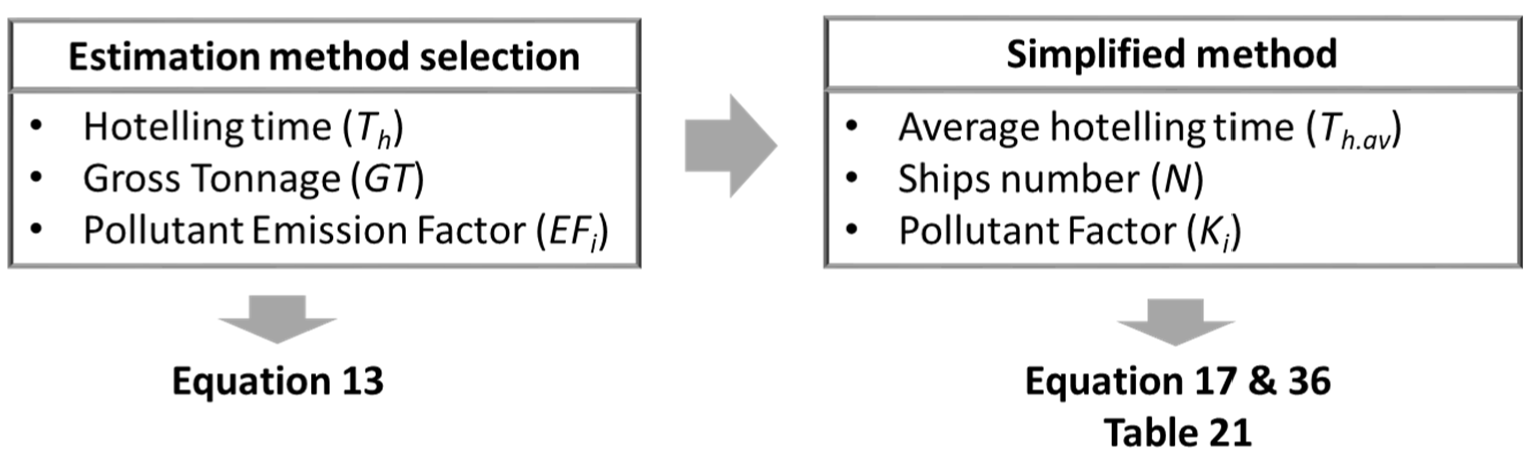
A summary of the methods proposed in this article is given in Figure 7.

This simplified method would be much faster and useful when making a first estimate of the total emissions from Ro–Ro ships in the Port of Vigo. It can perform both a global calculation, using the number of ships (N) that call at the port and the average hours of stay in hotels for all ships (T_h,av) (17), and per each pollutant (36), adding the corresponding factor (K_i) reflected in Table 21.

5. Conclusions

This article has provided a bibliographical review of the existing methods for estimating the emissions of ships in port, depending on the power of their auxiliary engines and fuel consumption. As a result, the most relevant methods have been applied to the particular case of Ro–Ro ships in the Port of Vigo, which has allowed them to be compared. In both cases, since the power of the auxiliary engines and fuel consumption are unknown, these methods estimate them by means of regression curves, based on a characteristic parameter of the vessel such as gross tonnage (GT).

Based on the analysis carried out, the best option selected in this article is the methodology for estimating emissions by means of auxiliary engine power according to 2010 World fleet [5]. From this methodology, the emissions of Ro–Ro ships during their stay in port are obtained on the basis of GT by using Equation (13).

However, once the total emissions have been obtained, it can be seen that the weightiest parameter in the calculation is the number of hours for hoteling of a ship in port (T_h), instead of GT, and that the emissions increase as the number of hours increases (Figure 6).

Consequently, a simplified estimation of total emissions from Ro–Ro ships during their stay in port was proposed, using the linear regression curve specified in Equation (17), as a function of the average value of hours for hoteling of ships in port (T_h,av) and number of ships (N).

Furthermore, if an estimation is required for the different pollutant types, this article proposes Equation (36), which adds a K factor corresponding to each pollutant (Table 21).

These equations are considered to be a potentially very useful and fast tool for obtaining the pollutant emissions of Ro–Ro ships during their stay in port.

However, this article has some limitations. In the follow-up carried out on the 50 ships that called in the port between July 2021 and March 2022, only sixteen ships have had some regularity and a relevant level of activity according to criteria established in Section 3.1.

Therefore, the procedure followed with Ro–Ro ships could also be applied to more Ro–Ro ships or other ship types, for which regression curves as a function of GT can also be found in the bibliography consulted and extrapolated for use in other ports.

Another limitation is when auxiliary engine power or fuel consumption are not known. Although it is the basis of this article, it could also be interesting to compare the results obtained with real data.

References

- State Ports. Guide to Energy Management in Ports; State Ports: Madrid, Spain, 2012; p. 296. (In Spanish) [Google Scholar]
- Yigit, K.; Acarkan, B. A new electrical energy management approach for ships using mixed energy sources to ensure sustainable port cities. Sustain. Cities Soc. 2018, 40, 126–135. [Google Scholar] [CrossRef]
- Kumar, J.; Kumpulainen, L.; Kauhaniemi, K. Technical design aspects of harbour area grid for shore to ship power: State of the art and future solutions. Int. J. Electr. Power Energy Syst. 2019, 104, 840–852. [Google Scholar] [CrossRef]
- ICF International. Current Methodologies in Preparing Mobile Source Port-Related Emission Inventories; Browning, L., Hartley, S., Facanha, C., Eds.; Final Report; U.S. Environmental Protection Agency: Washington, DC, USA, 2009; pp. 1–18. [Google Scholar]
- Trozzi, C. Emission Estimate Methodology for Maritime Navigation. In Proceedings of the US EPA 19th International Emissions Inventory Conference, San Antonio, TX, USA, 27–30 September 2010. [Google Scholar]
- Winkel, R.; Weddige, U.; Johnsen, D.; Hoen, V.; Papaefthimiou, S. Shore Side Electricity in Europe: Potential and environmental benefits. Energy Policy 2019, 88, 584–593. [Google Scholar] [CrossRef]
- Toscano, D.; Murena, F. Atmospheric ship emissions in ports: A review. Correlation with data of ship traffic. Atmos. Environ. X 2019, 4, 100050. [Google Scholar] [CrossRef]
- Bojić, F.; Gudelj, A.; Bošnjak, R. Port-Related Shipping Gas Emissions—A Systematic Review of Research. Appl. Sci. 2022, 12, 3603. [Google Scholar] [CrossRef]
- European Maritime Safety Agency (EMSA) and European Enviroment Agency (EEA). European Maritime Transport Environmental Report 2021; European Maritime Safety Agency (EMSA) and European Enviroment Agency (EEA): Lisbon, Portugal, 2021. [Google Scholar]
- International Maritime Organization. Annex VI of MARPOL Convention. In Prevention of Air Pollution from Ships; International Maritime Organization: London, UK, 1997. [Google Scholar]
- International Maritime Organization. Amendments Annex VI of MARPOL Convention. In Prevention of Air Pollution from Ships; International Maritime Organization: London, UK, 2021; Volume 328, Number 76. [Google Scholar]
- European Union. Directive (EU) 2016/802 of the European Parliament and of the Council of 11 May 2016 relating to a reduction in the sulphur content of certain liquid fuels. Off. J. Eur. Union 2016, 50, 58–78. [Google Scholar]
- European Union. Regulation (EU) 2015/757 of The European Parliament and of the Council of 29 April 2015 on the monitoring, reporting and verification of carbon dioxide emissions from maritime transport, and amending Directive 2009/16/EC. Off. J. Eur. Union 2015, 58, 55–76. [Google Scholar]
- European Commission. The European Green Deal; European Commission: Brussels, Belgium, 2019; p. 24. [Google Scholar]
- European Union. Regulation (EU) 2021/1119 of The European Parliament and of the Council of 30 June 2021 establishing the framework for achieving climate neutrality and amending Regulations (EC) No 401/2009 and (EU) 2018/1999 (“European Climate Law”). Off. J. Eur. Union 2021, 243, 1–17. [Google Scholar]
- European Commission. Fit for 55: Delivering the EU’s 2030 Climate Target on the Way to Climate Neutrality; European Commission: Brussels, Belgium, 2021; p. 15. [Google Scholar]
- Marinello, S.; Balugani, E.; Rimini, B. Sustainability of logistics infrastructures: Operational and technological alternatives to reduce the impact on air quality Sustainability of logistics infrastructures: Operational and technological alternatives to reduce the impact on air quality. In Proceedings of the Summer School Francesco Turco, Online, 8–10 September 2021. [Google Scholar]
- Perčić, M.; Ančić, I.; Vladimir, N. Life-cycle cost assessments of different power system configurations to reduce the carbon footprint in the Croatian short-sea shipping sector. Renew. Sustain. Energy Rev. 2020, 131, 110028. [Google Scholar] [CrossRef]
- Fan, L.; Xiao, C.; Chao, X.; Zhang, H.; Lu, Y.; Song, E. Energy Efficiency Analysis of Parallel Ship Gas-Battery Hybrid Power System. In Proceedings of the ICTIS 2019—5th International Conference on Transportation Information and Safety, Liverpool, UK, 14–17 July 2019; pp. 1111–1116. [Google Scholar]
- Sanabra, M.C.; Santamaría, J.J.U.; De Osés, F.X.M. Manoeuvring and hotelling external costs: Enough for alternative energy sources? Marit. Policy Manag. 2014, 41, 42–60. [Google Scholar] [CrossRef]
- Campisi, T.; Marinello, S.; Costantini, G.; Laghi, L.; Mascia, S.; Matteucci, F.; Serrau, D. Locally integrated partnership as a tool to implement a Smart Port Management Strategy: The case of the port of Ravenna (Italy). Ocean Coast. Manag. 2022, 224. [Google Scholar] [CrossRef]
- Nunes, R.A.O.; Alvim-Ferraz, M.C.M.; Martins, F.G.; Sousa, S.I.V. The activity-based methodology to assess ship emissions—A review. Environ. Pollut. 2017, 231, 87–103. [Google Scholar] [CrossRef] [PubMed]
- Vigo Port Authority—Commercial Port. 2022. Available online: https://www.apvigo.es/es/paginas/presentacion_puerto_comercial (accessed on 27 October 2022).
- Inovalabs. Agile Innovation “Study of The Feasibility of Implementing OPS Systems in the Port of Vigo”. In Analysis for the Ro-Ro Terminal; Inovalabs: Vigo, Spain, 2019. (In Spanish) [Google Scholar]
- Inovalabs. Agile Innovation “Study of the feasibility of implementing OPS systems in the Port of Vigo”. In Analysis for the Transatlantic Terminal; Inovalabs: Vigo, Spain, 2019; p. 48. (In Spanish) [Google Scholar]
- Schrooten, L.; De Vlieger, I.; Panis, L.I.; Styns, K.; Torfs, R. Inventory and forecasting of maritime emissions in the Belgian sea territory, an activity-based emission model. Atmos. Environ. 2008, 42, 667–676. [Google Scholar] [CrossRef]
- Wang, C.; Corbett, J.J.; Firestone, J. Modeling Energy Use and Emissions from North American Shipping: Application of the Ship Traffic, Energy, and Environment Model. Environ. Sci. Technol. 2007, 41, 3226–3232. [Google Scholar] [CrossRef] [PubMed]
- Trozzi, C.; Vaccaro, R. Actual and Future Air Pollutant Emissions from Ships. In Proceedings of the Transport and Air Pollution and Cost, Graz, Austria, 31 May–2 June 1999. no. 319. [Google Scholar]
- Izzaty, R.E.; Astuti, B.; Cholimah, N. Methodology for Calculating Transport Emissions and Energy Consumption; European Commission: Brussels, Belgium, 1999; p. 408. [Google Scholar]
- Trozzi, C.; Vaccaro, R. Air Pollutant Emissions from Ships: High Tyrrhenian Sea Ports Case Study. In Proceedings of the 1st International Conference PORTS 98 Maritime Engineering and Ports, Genoa, Italy, 28–30 September 1998; p. 11. [Google Scholar]
- Saputra, H.; Muvariz, M.F.; Satoto, S.W.; Koto, J. Estimation of exhaust ship emission from marine traffic in the straits of Singapore and batam waterways using automatic identification system (AIS) data. J. Teknol. 2013, 77, 47–53. [Google Scholar] [CrossRef]
- Fuentes, G.G.; Sosa, E.R.; Baldasano, R.J.M.; WKahl, J.D.; Antonio, D.R. Review of Top-Down Method to Determine Atmospheric Emissions in Port. Case of Study: Port of Veracruz, Mexico. J. Mar. Sci. Eng. 2022, 10, 96. [Google Scholar]
- Lucialli, P.; Ugolini, P.; Pollini, E. Harbour of Ravenna: The contribution of harbour traffic to air quality. Atmos. Environ. 2007, 41, 6421–6431. [Google Scholar] [CrossRef]
- Trozzi, C.; Vaccaro, R. Methodologies for Estimating Future Air Pollutant Emissions from Ships: A 2006 update. In Proceedings of the 2th International Scientific Symposium, Reims, France, 12–14 June 2006; p. 8. [Google Scholar]
- vesseltracker.com. 2022. Available online: https://www.vesseltracker.com/ (accessed on 28 March 2022).
- Maritime Transport Research Group; EnerTrans. Energy Consumption and Emissions Associated with Ship Transport; University of Oviedo: Oviedo, Spain, 2019; Volume 15. (In Spanish) [Google Scholar]
- Entec. Entec Defra UK Ship Emissions Inventory; Final Report; Entec UK: London, UK, 2010; p. 168. [Google Scholar]
- Entec. Quantification of Emissions from Ships Associated with Ship Movements between Ports in the European Community Final Report; Entec UK: Cheshire, UK, 2002; p. 59. [Google Scholar]
- Styhre, L.; Winnes, H. Emissions From Ships in Ports. In Green Ports: Inland and Seaside Sustainable Transportation Strategies; Bergqvist, R., Monios, J., Eds.; Elsevier: Amsterdam, The Netherlands, 2018; pp. 109–124. [Google Scholar]
- Environmental Protection Agencgy. Inventory Guidance: Ports Emissions Inventory Guidance; Environmental Protection Agency: Washington, DC, USA, 2021. [Google Scholar]
- Starcrest Consulting Group LLC. San Pedro Bay Ports Emission Inventory Methodology Report; Starcrest Consulting Group LLC: Albuquerque, NM, USA, 2019; Volume 1, p. 43. [Google Scholar]
- Starcrest Consulting Group LLC. Port of Los Angeles. Inventory of Air Emissions—2020; Starcrest Consulting Group LLC: Albuquerque, NM, USA, 2021; p. 114. [Google Scholar]
- Trozzi, C.; De Lauretis, R. EMEP/EEA Air Pollutant Emission Inventory Guidebook 2019; Publications Office of the European Union: Luxembourg, 2019. [Google Scholar]
- Goldsworthy, L.; Goldsworthy, B. Modelling of ship engine exhaust emissions in ports and extensive coastal waters based on terrestrial AIS data—An Australian case study. Environ. Model. Softw. 2015, 63, 45–60. [Google Scholar] [CrossRef]
- MarineTraffic. 2022. Available online: https://www.marinetraffic.com (accessed on 28 March 2022).
- VesselFinder. 2022. Available online: https://www.vesselfinder.com/ (accessed on 28 March 2022).
Figure 1.
Methods to estimate emissions from ships in port [
5,
26,
27,
28,
29,
30,
31,
32,
33,
34,
35,
36].
Figure 2.
Ro–Ro terminal location in Port of Vigo. Source: Google Earth, 2020.
Figure 3.
Auxiliary engines’ consumed power (kW) in comparison with load factor of 0.4.
Figure 4.
Fuel consumption comparison through the Trozzy and Vaccaro, Schrooten and Goldsworthy, and Fuentes García methods.
Figure 5.
Common polluting emissions percentages of the Ro–Ro ships in the Port of Vigo.
Figure 6.
Influence analysis of the time for hoteling (Th) and GT in the emissions calculation.
Figure 7.
Summary of proposed methods.