Study of Overtopping Flow Velocity and Overtopping Layer Thickness on Composite Breakwater under Regular Wave

Abstract

Overtopping flow velocity (OFV) and overtopping layer thickness (OTL) are essential parameters in breakwater design. Several empirical equations to predict these parameters are available in many works of literature, but most of the equations were derived based on impermeable structures such as sea dikes. In this study, we experimented with overtopping waves over a composite breakwater with tetrapod armor units. In the experiments, wave overtopping was generated from regular waves. We used a digital image-based velocimetry method, bubble image velocimetry (BIV), to measure the OFV and digitize the corresponding image to obtain the OLT. The patterns of OFV and OTL with respect to time steps, wave conditions, and corresponding events were provided and discussed. The application of the widely used empirical equations for sea dike to breakwater was also tested by calibrating the coefficients. New empirical coefficients and roughness factors were suggested to reduce the difference between predicted and measured OFV and OLT on breakwater through the bootstrap resampling technique. This study provides modified empirical equations on wave overtopping, which is further applicable to breakwater design.

1. Introduction

Wave overtopping occurs when the wave run-up is higher than the crest freeboard. Wave overtopping transfers the wave energy to the crest and rear side of the coastal defense structure. It affects the stability of the structure’s crest and rip rap structure [1]. Moreover, the wave overtopping flow poses a threat to the safety of pedestrians since the crest of the structures is often used as a recreation place. As reported in EurOtop [2], in 2015, 11 people died due to wave overtopping or wave action on a coastal structure in UK. In addition, global warming leads to sea level rise, and stronger wave storms may exacerbate the wave overtopping hazard. The recent studies by Gao et al. [3,4] also show that long-period coastal waves have significant adverse effects on wave overtopping. It is not feasible to avoid wave overtopping due to the cost of an uneconomical high coastal defense structure. Therefore, it is essential to estimate wave overtopping flow behavior accurately.

Wave overtopping flows can be characterized by wave overtopping flow velocity (OFV) and wave overtopping layer thickness (OLT). These parameters are considered important when pedestrian safety on a coastal defense structure is a priority. There is extensive literature focused on OFV and OLT on sea dike crests, e.g., van Gent [5], Schüttrumpf [6], and van der Meer et al. [7]. These studies have proposed empirical design formulas to predict OFV and OLT, which are collected in the EurOtop [2] manual. Several studies also have investigated the tolerable limits for OFV and OLT to ensure pedestrian safety under overtopping flow on vertical wall structures. For example, Bae et al. [8] and Cao et al. [9]. studied the tolerable limits for these parameters on vertical wall structures. However, a few studies have focused on OFV and OLT on armored breakwater crests [10,11,12].

A breakwater is typically constructed in areas where water waves are severe and at high risk of wave overtopping. Existing empirical formulas used for predicting OFV and OLT on sea dikes can serve as the basis for predictions on breakwater crests. In the empirical design equations, there are reduction factors and empirical coefficients that depend on hydraulic and geometrical conditions. These variables need to be calibrated with experimental data to improve estimation accuracy [13,14]. An example of this approach is presented in Mares-Nassare et al. [10], where they adopted and calibrated existing empirical formulas on sea dikes proposed by Schüttrumpf and van Gent [15] and EurOtop [2]. They also introduced a new formula for estimating OLT on rubble mound breakwaters. OFV was estimated from the measured OLT at the middle of the crest. As suggested by Pepi et al. [14], further research is still required for different hydraulic and structure geometries.

In this study, we investigated the OFV and OLT on a composite breakwater through physical experimentation. We adopted and calibrated the existing prediction formula for the sea dike and proposed new empirical coefficients and reduction factors to extend the application of the empirical equation for OFV and OLT estimation on the breakwater. Unlike common measurement techniques for OFV and OLT, such as micro propeller and wave gauge, this study used a digital imaging technique to measure the wave overtopping flow parameters and understand the flow behavior from spatial distribution as well as temporal change.

The paper is organized as follows. Section 2 presents a literature review of previous studies on OFV and OLT. In Section 3, we describe the physical experiment setup and the measurement technique. Section 4 provides a comparison of the measured OFV and OLT with the estimation using the existing empirical equations as well as relationships of the parameters. Additionally, we provide flow patterns and the application of the new empirical coefficients and reduction factors in different wave conditions and structure geometries in this section. The interpretation of the results is discussed in Section 5. Finally, we draw a conclusion in Section 6.

2. Literature Review

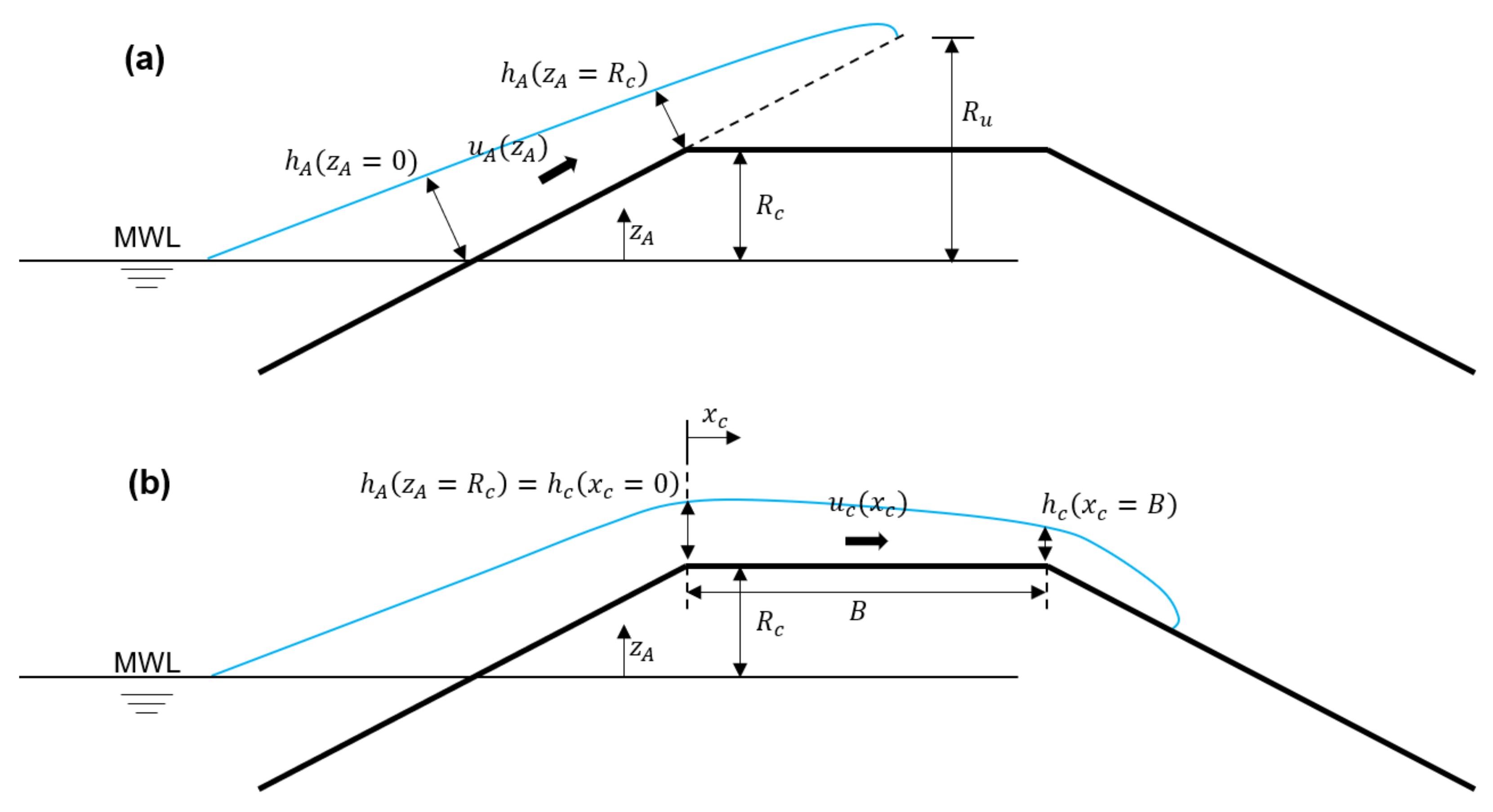
Wave overtopping occurs when the wave run-up height, $R_u$, exceeds the structure crest freeboard, $R_c$. The wave run-up height is a vertical difference between the highest point of wave run-up and the mean water level (MWL). Wave run-up height can be calculated for the situation where the crest freeboard is high enough to prevent wave overtopping. During wave overtopping, the crest freeboard height is less than the wave run-up height. In that condition, the seaward slope is virtually extended to allow considering a fictitious wave run-up level, as shown in Figure 1a. This fictitious wave run-up on a sea dike structure was investigated by van Gent [16] through a prototype measurement for physical model testing and numerical modeling, and Equation (1) was proposed to estimate the fictitious wave run-up height:

$$\begin{gathered} \frac{R_u}{H_s}=c_0\xi \mathrm{if} \xi \le p, \\ \frac{R_u}{H_s}=c_1-\frac{c_2}{\xi } \mathrm{if} \xi \ge p, \end{gathered}$$

(1)

where $c_0$ = 1.35, $c_1$ = 4.7, $c_2$ is given by Equation (2), $p$ is given by Equation (3), $H_s$ is the significant wave height of the incident wave height at the toe of the structure, and $\xi$ is the surf similarity or Iribarren number given by Equation (4).

$$c_2=0.25\frac{c_1^2}{c_0},$$

(2)

$$p=0.5\frac{c_1}{c_0},$$

(3)

$$\xi =\frac{\tan \alpha }{\sqrt{2\pi H_s/T^2}}$$

(4)

where T is the spectral wave period and $\alpha$ is the seaward structure slope.

Van Gent [5] and Schüttrumpf et al. [6] performed an experiment focusing on the measurement of OFV and OLT on sea dikes. van Gent [5] carried out a small-scale experiment using a sea dike with a single seaward slope $V/H=$ 1/4, and Schüttrumpf et al. [6] used a dike with three different seaward slopes, $V/H=$ 1/3, 1/4, and 1/6. In addition, Schüttrumpf et al. [6] also conducted a large-scale experiment to confirm the small-scale experiment result. In van Gent [5], the wave run-up parameters were estimated based on a fictitious wave run-up height calculated using Equations (1)–(4), while, in Schüttrumpf et al. [6], the wave run-up parameters were derived from measured wave run-up height. van Gent [5] and Schuttrumpf et al. [6] combined the findings in Schüttrumpf and van Gent [15] and proposed Equations (5) and (6) to estimate the wave run-up parameters on the seaward slope of the sea dike.

$$u_A=c_{A,u}\left(\sqrt{\mathrm{g}\left(R_u-z_A\right)}\right),$$

(5)

$$h_A=c_{A,h}\left(R_u-z_A\right),$$

(6)

where $u_A$ is the wave run-up velocity; $h_A$ is the wave run-up layer thickness; $z_A$ is the elevation from the MWL; and $c_{A,u}$ and $c_{A,h}$ are the empirical coefficients given in

Table 1. Range of the applicability and empirical coefficients from the previous studies.

	van Gent [5]	Schüttrumpf et al. [6]	van der Meer et al. [7]	EurOtop [2]	Mares-Nasarre et al. [10]
Structure	Sea dike	Sea dike	Sea dike	Sea dike	Breakwater
$\mathrm{Slope} (V/H$)	1/4	1/3, 1/4, 1/6	1/3	1/3, 1/4, 1/6	2/3
$R_c/H_s$	0.7–2.2	0.0–2.5	0.7–2.9	-	0.34–1.75
$c_{A,u}$	1.30	1.37	$0.35\cot \alpha$	1.4, 1.5	-
$c_{A,h}$	0.15	0.33	0.19	0.20, 0.30	0.52
$c_{c,u}$	0.50	0.50	-	-	-
$c_{c,h}$	0.40	0.89	0.13	-	-

. The transition line between the seaward slope and crest is the initial condition for the wave overtopping flow on the crest. The overtopping flow parameters at this point can be estimated using Equations (5) and (6), with $z_A=R_c$ (Figure 1b). Schüttrumpf and van Gent [15] also proposed a method to estimate the wave overtopping flow parameters, OFV ($u_c\left(x_c\right)$) and OLT ($h_c\left(x_c\right)$), along the dike crest using Equations (7) and (8):

$$\frac{u_c\left(x_c\right)}{u_A\left(R_c\right)}=\exp \left(-c_{c,u}\frac{x_c\mu }{h_c\left(x_c\right)}\right),$$

(7)

$$\frac{h_c\left(x_c\right)}{h_A\left(R_c\right)}=\exp \left(-c_{c,h}\frac{x_c}{B}\right),$$

(8)

where $x_c$ is the distance from the intersection of the crest and seaward slope; $B$ is the crest width; $\mu$ is the friction coefficient; and $c_{c,u}$ and $c_{c,h}$ are the empirical coefficients given in Table 1.

As seen in Table 1, the empirical coefficient for wave run-up layer thickness, $c_{A,h}$, given by Schüttrumpf et al. [6], is about 2 times larger (i.e., 2.2) than that by van Gent [5]. They proposed a different empirical coefficient based on their own experimental results. This led to different results on the estimation of OLT, as shown in Mares-Nasarre et al. [10]. According to Schüttrumpf and van Gent [15], the discrepancy between these empirical coefficients was due to the different dike geometries and instruments they used. Bosman et al. [17] investigated the discrepancy of these empirical coefficients through a physical experiment. Two different dike geometries, $V/H=$ 1/4 and $V/H=$ 1/6 were used, with one wave condition for both dikes. They found that the seaward slope of the structure influences these empirical coefficients. Later, Lorke et al. [18] conducted a physical experiment that measured the OFV and OLT at the seaward crest edge and landward crest edge using wave gauges and micro propellers. The authors also proposed new empirical coefficients based on the seaward slope of the structure.

Van der Meer et al. [7] conducted a physical test on a dike with a slope $V/H=$ 1/3 and measured the OFV and OLT at the seaward crest edge and landward crest edge. In their study, they combined their experimental results with the observation from van Gent [5] and Schüttrumpf et al. [6]. Based on this newly combined data, van der Meer et al. [7] proposed Equation (9) to estimate $u_A$at the seaward crest edge with a slightly different empirical coefficient, $c_{A,u}$, as shown in Table 1. The $u_c$ along the dike crest is then estimated as the decay function given by Equation (10):

$$u_A\left(z_A=R_c\right)=c_{A,u}\left(\sqrt{\mathrm{g}\left(R_u-z_A\right)}\right),$$

(9)

$$\frac{u_c\left(x_c\right)}{u_A\left(R_c\right)}=\exp \left(-1.4\frac{x_c}{L}\right),$$

(10)

where $L$ is the wavelength based on the spectral wave period. The empirical coefficient in Equation (9) is $c_{A,u}=0.35\cot \alpha$, meaning that the slope angles of the structure is taken into account in the prediction. van der Meer et al. [7] also proposed Equation (11) to estimate $h_c$ along the sea dike crest:

$$h_c\left(x_c\right)=c_{c,h}\left(R_u-R_c\right).$$

(11)

Based on their analysis, OLT decreases directly behind the seaward crest edge and then remains almost constant along the crest. The wave run-up layer thickness at the seaward edge, $h_A$, is 50% larger than $h_c$ gave in Equation (11).

Based on the aforementioned studies, it can be concluded that the wave overtopping flow parameters along the crest can be estimated based on the wave run-up parameters at the seaward crest together with the empirical coefficient. However, since the seaward slope of the sea dike is impermeable and smooth, the estimation of a fictitious wave run-up height formula using Equations (1)–(4) is not applicable for rough slopes such as breakwater structures. EurOtop [2] provided an empirical formula to estimate the fictitious wave run-up on the armored front slope of a structure such as a breakwater using Equation (12):

$$\frac{R_u}{H}=1.65\cdot {\gamma }_f\cdot {\gamma }_{\beta }\cdot {\gamma }_b\cdot \xi ,$$

(12a)

with the maximum value of

$$\frac{R_u}{H}=1·{\gamma }_{fsurging}·{\gamma }_{\beta }·\left(4.0-\frac{1.5}{\sqrt{{\gamma }_b·\xi }}\right),$$

(12b)

where ${\gamma }_f$ is the influence of roughness of the slope; ${\gamma }_{\beta }$ is the influence of oblique wave attack; ${\gamma }_b$ is the influence of berm; ${\gamma }_{fsurging}$ is a coefficient of ${\gamma }_f$ when $\xi >$1.8:

$${\gamma }_{fsurging}={\gamma }_f+\left(\xi -1.8\right)\frac{1-{\gamma }_f}{8.2}.$$

(13)

In the case of an impermeable and smooth seaward slope structure, where the wave attack is perpendicular to the structure without a berm, the roughness factor, ${\gamma }_f$, the influence of oblique wave attack, ${\gamma }_{\beta }$, and the influence of the berm, ${\gamma }_b$, are equal to 1. The ${\gamma }_f$ value for different types of armor units can be found in [2]. For 2 layered tetrapods on a rubble mound breakwater with a permeable core, they derived ${\gamma }_f=$ 0.42.

EurOtop [2] adopted Equations (5) and (6) to estimate the wave run-up parameters, wave run-up velocity, $u_A$, and wave run-up layer thickness, $h_A$. As shown in Table 1, EurOtop [2] specifies the empirical coefficient $c_{A,u}=$ 1.4 for the slope 1/3 and 1/4 and $c_{A,u}$ = 1.5 for the slope of 1/6. In the case of the seaward structure slope between these values, EurOtop [2] suggested applying interpolation to obtain the empirical coefficient. Similarly, EurOtop [2] also provided the empirical coefficient $c_{A,h}=$ 0.20 for the of slope 1/3 and 1/4 and $c_{A,h}=$ 0.30 for the slope of 1/6 and suggested an interpolation method to obtain an empirical coefficient between these slopes. The OFV along the crest was then estimated using Equation (10). According to EurOtop [2], the OLT along the crest was 2/3 of that at the seaward crest edge ($h_c$($x_c$>>0)) = $2/3·h_A$($R_c$)).

Recently Mares-Nasarre et al. [10] conducted an experiment on a mound breakwater with the seaward slope $V/H=$ 2/3, focusing on OFV and OLT at the middle of the crest. Mares-Nasarre et al. [10] used Equation (12) proposed by EurOtop [2] to estimate the fictitious wave run-up height on three different armor units: 1-layer cubipod, 2-layers rock, and 2-layers cube. The wave run-up layer thickness at the seaward crest edge ($h_A(z_A=R_c$)) and at the middle of the crest ($h_c(x_c$ = B/2)) was estimated using Equations (6) and (8). They calibrated the roughness factor, ${\gamma }_f$, and empirical coefficient, $c_{A,h}$, with their experiment data following procedures given in Molines and Medina [13] and proposed a new empirical coefficient, as shown in Table 1.

According to Molines and Medina [13] the roughness factor, ${\gamma }_f$, is a fitting parameter and needs to be calibrated based on the database. Pepi et al. [14] proposed a new formula to calculate the roughness factor for 2-layers rock mound breakwater with the seaward slope $V/H=$ 1/2. Calibration of ${\gamma }_f$, as well as the empirical coefficient, reduced the difference between measured and estimated wave overtopping parameters [10,13,14]. This indicates that using the available empirical equation with a calibrated empirical coefficient and roughness factor has a potential application in the estimation of wave overtopping flow parameters on different coastal defense structures. Hence, in this paper, we extend the application of the empirical equation. We adopted Equation (12) to estimate the fictitious wave run-up height on the breakwater with 2-layers tetrapods and a permeable core. Then the wave run-up parameters were estimated using Equations (5) and (6). Finally, the OFV was estimated using Equation (10), and the OLT was estimated as $h_c$($x_c$>>0)) = $2/3·h_A$($R_c)$ [2]. The roughness factor and empirical coefficient were calibrated following the method presented by Molines and Medina [13] and Mares-Nasarre et al. [10].

3. Materials and Methods

3.1. Experiment Setup

The experiment was performed in a two-dimensional wave flume, as shown in Figure 2. The wave flume is 56 m long, 1 m wide, and 2 m high with a transparent side wall. The wave flume is equipped with a piston-type wave maker located 5 m from the end of the flume and can produce regular and irregular waves. The 1:37.5 sloping beach starts 19 m from the wave maker, and the horizontal beach with the layer of horsehair is at the other end of the tank to absorb wave energy and reduce reflection. The wave flume was split into two sections (0.6 m to 0.4 m). The wide section was used to place the breakwater model, and the narrow section was used to measure the incident wave without being affected by the reflection from the structure model.

The model of the composite-type breakwater (scale 1/40) was located 34.5 m away from the wave maker. The model structure consists of a caisson in the middle, armor layers on the front side, and no structure on the rear side (Figure 3). The caisson model structure has a height of 0.52 m, a length of 0.55 m and a width of 0.33 m. The water depth at the structure was kept constant at $d=$ 0.40 m, and the freeboard ($R_c$) was 0.12 m. On the front side, the armor layers consist of three layers. First, the outer layer with the slope $V/H=$ 1:1.5 was constructed with two layers of tetrapod (TTP) armor units. The TTP has a mass of $M=$ 307 g and a layer thickness of 0.107 m. The second layer is the filter layer, made from natural rocks with a diameter $D_{n50}=$ 0.08 m, a mass $M=$ 85 g, and a layer thickness of 0.03 m. The third layer is the core layer made from quarry rock with a diameter $D_{n50}=$ 0.012 m and a mass $M=$ 10–12 g. The armor layers are the same height as the caisson part. On the crest, the TTP layer has a width of 0.22 m, and the total width of the structure is 0.55 m. In order to be representative of the general situation, the design of the structure was intended to be as simple as possible in terms of geometrical configuration. The shape of the structure, especially the armored front section, has been checked after each test to verify the constancy of the geometrical parameters.

The water surface elevation was measured using five capacitance-type wave gauges. Two gauges (named G2 and G3) were installed in the wide section 19 m downstream from the wave maker to monitor the generated waves. In the wide and narrow sections of the flume, two wave gauges (named G4 and G5) were installed 34 m downstream from the wave maker to determine the waves with and without the structure at the breakwater toe. The fifth gauge, G6, was installed behind the breakwater to monitor the transferred wave.

Table 2. Test conditions.

Description	Parameter	Ranges
Wave period	$T$	1.5–3.0 s
Wave height	$H$	0.12–0.20 m
Relative water depth	$d/L$	0.028–0.114
Wave steepness	$H/L$	0.008–0.057
Iribarren’s number	$\xi$	2.795–7.216
Relative crest freeboard	$R_c/H$	0.6–1

presents the test conditions of the current experiment. The regular wave was used in this experiment since the direct relationship between wave condition and wave overtopping flow parameters can be analyzed. The regular waves have a wave period ($T$) of 1.5–3.0 s and a wave height ($H$) of 0.12–0.20 m. These wave components represent the wave conditions, including storm conditions. The water wave conditions at the breakwater toe are determined by the relative water depth, $d/L$, where $L$ is the wavelength from the dispersion relationship. The relative water depth conditions were in the range of 0.028–0.114, indicating shallow to intermediate water depth. The waves were non-breaking waves, as the wave steepness, $H/L$, was in the range of 0.008–0.057. The Iribarren’s number or the breaker parameter in this study, $\xi =\tan \alpha /\sqrt{H/L}$, was in the range of 2.795–7.216, showing a collapsing to surging wave. The relative crest freeboard, $R_c/H$, was in the range of 0.6–1, and the wave overtopping was observed in all relative crest freeboard conditions.

In the experiment, some of the wave energy is reflected by the breakwater. These reflected waves are re-reflected towards the breakwater and lead to increasing wave height. Therefore, the measurements are only valid after the unstable part of the initial wave and before the leading edge of the re-reflected wave reaches the breakwater. In this study, the valid measurement time was defined as the arrival time between the first fully developed wave and the first re-reflected wave at the breakwater toe. By limiting the measurement time of the wave overtopping parameters, OFV and OLT, the reflection would not affect the result. From the comparison of the free surface elevations from G4 and G5, available wave components close to the target wave were selected for the analysis.

3.2. Overtopping Flow Velocity and Layer Thickness Measurement

When the wave flows overtop the breakwater structure, the flows usually contain a lot of bubbles. These bubbles make the existing velocity measurement equipment less accurate. In this study, a flow visualization technique called bubble image velocimetry (BIV) was applied to estimate the velocity of the overtopping flows. The BIV technique was first introduced by Ryu et al. [19]. This technique has the same principle as particle image velocimetry (PIV) with a flow visualization and digital image analysis to estimate the flow velocity. However, the PIV technique does not work well in multi-phase flows, such as overtopping flows, where the flows contain a lot of bubbles, due to the air–water interface, which will scatter the laser light. On the other hand, the BIV technique uses these bubbles within the flows as a tracer. These bubble textures in overtopping flow are visualized by means of a shadowgraphy technique and then captured by a high-speed camera. The measurement location in this technique is determined by adjusting the depth of field (DOF). The texture of the bubbles will appear sharp within the DOF and blurry on the outside (Figure 4a). A pair of overtopping flow images were captured by a high-speed camera and then analyzed using a cross-correlation method similar to the PIV technique in order to calculate the velocity.

Figure 4 shows the BIV technique set up and the camera field of view (FOV). A Photron high-speed camera system, FASTCAM Mini UX50, was used in this study. This camera has a CMOS image sensor with a maximum resolution of 1280 $\times$ 1024 pixels, a 12-bit dynamic range, a maximum frame rate of 2000 frames per second (fps), a maximum shutter speed of 1/256,000 s, and an internal memory capacity of 8 GB. The camera was equipped with AF Micro Nikkor 60 mm lens. In this study, the camera was placed 3.5 m from the measurement plane, and the FOV covered the rear part of the breakwater model where the overtopping flow falls and plunges into the rear water surface. The camera resolution was set at 1280 $\times$ 720 pixels, 8-bit dynamic range, and the lens aperture was set at the f-number of 2.8, yielding the 0.584 $\times$0.584 mm² spatial resolution. After several preliminary tests, the camera framing rate was set at 500 fps, and the interval between two consecutive images ($\Delta t$) was 2 ms.

The open-source software called PIVlab developed by Thielicke and Stamhuis [20] was used to analyze BIV images and calculate the velocities. Raw images were firstly inverted so that high-intensity (brightness) represents bubbles. A multi-pass algorithm with an initial window size of 32 $\times$ 32 pixels and a final window size of 16 $\times$ 16 pixels was employed with a 50% overlap between adjacent windows. Note that the estimated mean maximum bubble diameter of 12 pixels is about 3/4 of the final window size. A cross-correlation was then applied to compute velocity vectors. A median filter was used to remove spurious vectors and boundary values, and then interpolation was applied to fill the removed bad vectors. Figure 5 shows the snapshot of the velocity map of the overtopping flow passing the rear edge of the breakwater crest captured using the setup in Figure 4.

In this study, the OFV is the horizontal velocity at the rear edge of the breakwater crest obtained from the velocity map and is denoted as $u_m$. The OLT, $h_m$, was obtained from the digital image at the same location as the $u_m$ by digitizing the water surface. Figure 6 shows the example of time series $u_m$ and $h_m$ from wave conditions $T=$ 2.75 s and $H=$ 16 cm. Both $u_m$ and $h_m$ have a pattern with a sudden increase to the maximum value at the beginning stage and a gradual decrease after that. The maximum $u_m$ value occurred first, followed by the maximum value of $h_m$. This indicates that the front body of wave overtopping flows possess the largest momentum with a huge velocity and a thick layer. The fluctuation of $u_m$ between 0.75 and 1.25 s is due to thin layer thickness and fewer air bubbles, which is considered to be an error. Nevertheless, for the analysis of $u_m$ and $h_m$ in the next section, the maximum values were selected.

3.3. Evaluation Metric

In this study, the measurement data and the estimation using Equations (5), (6), (10) and (12) were compared. The fitting of the estimation data was analyzed using the relative root mean squared (rRMSE) given by Equation (14) and the coefficient of determination (R²) given by Equation (15):

$$\mathrm{rRMSE}=\frac{\mathrm{RMSE}}{\mathrm{MEAN}}=\frac{\sqrt{\frac{{{\displaystyle \sum }}_{i=1}^N{\left(x_i-y_i\right)}^2}{N}}}{\overline{x}},$$

(14)

$$R^2=1-\frac{{{\displaystyle \sum }}_{i=1}^N{\left(x_i-y_i\right)}^2}{{{\displaystyle \sum }}_{i=1}^N{\left(x_i-\overline{x}\right)}^2},$$

(15)

where $x_i$ is the measured data; $\overline{x}$ is the average of the measured data; $y_i$ is the estimated data; and $N$ is the total amount of data. In addition, the correlation coefficient ($r$) was calculated using Equation (16), with $\overline{y}$ as the average estimated data.

$$r=\frac{{{\displaystyle \sum }}_{i=1}^N\left(x_i-\overline{x}\right)\left(y_i-\overline{y}\right)}{\sqrt{{{\displaystyle \sum }}_{i=1}^N{\left(x_i-\overline{x}\right)}^2{{\displaystyle \sum }}_{i=1}^N{\left(y_i-\overline{y}\right)}^2}},$$

(16)

4. Results

4.1. Overtopping Flow Velocity

4.1.1. Estimation of the Overtopping Flow Velocity

In this study, Equation (12) given by EurOtop [2] was used to estimate the fictitious wave run-up height. The wave run-up velocity at the seaward crest edge was estimated using Equation (5) given by Schüttrumpf and van Gent [15]. Finally, the OFV at the landward crest edge was estimated using Equation (10) given by van der Meer et al. [7]. Figure 7 shows the comparison between the measured OFV at the landward crest edge, $u_m$, and estimated OFV at the same point, $u_e$. The empirical coefficient and roughness factor used in the estimation were selected as $c_{A,u}=$ 1.3, given by van Gent [5], and ${\gamma }_f=$ 0.38, given by EurOtop [2]. The OFV estimations using the other empirical coefficients available in the literature and the roughness factor, ${\gamma }_f=$ 0.38, are shown in

Table 3. Quantitative results on the estimation of OFV using different empirical coefficients available in the previous studies.

Previous Studies	${\mathit{c}}_{\mathit{A},\mathit{u}}$	rRMSE
EurOtop [2]	1.50	0.273
	1.40	0.198
Schüttrumpf et al. [6]	1.37	0.177
van Gent [5]	1.30	0.134

. As we can see in Table 3, the best estimation was obtained when using the empirical coefficient given by van Gent [5] with rRMSE $=$ 0.134 with $R^2=$ 0.702. The other estimation gives a similar $R^2$ value because the scattered pattern of the data does not change dramatically with the change of the empirical coefficient, $c_{A,u}$.

According to Molines and Medina [13], the roughness factor, ${\gamma }_f$, is a fitting parameter where its value is different depending on the formula and database. In addition, the empirical coefficients were obtained from the experiment where the structure was a sea dike with a different seaward slope. Therefore, the empirical coefficient, $c_{A,u}$, and roughness factor, ${\gamma }_f$, need to be calibrated with the experiment data as well.

Using the empirical equation given in EurOtop [2] and the experimental data obtained in this study, an rRMSE can be used to estimate the optimum $c_{A,u}$ and ${\gamma }_f$, which minimizes the prediction error. However, no uncertainty information regarding the $c_{A,u}$ and ${\gamma }_f$ are obtained. To overcome the uncertainty of the estimation of the $c_{A,u}$ and ${\gamma }_f$, a bootstrap resample technique was used in this study [10,13]. In the bootstrap resampling technique, a new dataset called a bootstrapped dataset was created using a resample with a replacement from the original dataset; therefore, it had the same number of samples as the original dataset. Then the mean value of bootstrapped dataset was calculated. This process was repeated several times, and the distribution of mean values was obtained.

Since there were two variables in this study, the resampling procedure shown in Mares-Nassare et al. [10] was followed. The procedure has two levels of bootstrap resampling. Firstly, 1000 resamplings were performed by optimizing both the roughness factors and the empirical coefficients. Thus, 1000 mean values of roughness factors and empirical coefficients that minimize the rRMSE were obtained, and the mean values were used to statistically characterize the parameters using percentiles of 5%, 50%, and 95%. Figure 8a shows the histogram of the empirical coefficient, $c_{A,u}$, obtained from the first level bootstrap. The P5%, P50%, and P95% were 1.18, 1.21, and 1.24, respectively.

On the second level of bootstrap resampling, the empirical coefficient value was fixed at the 50% percentile ($c_{A,u}$ = 1.21), and 1000 resamples were performed by varying the roughness factor, ${\gamma }_f$. The optimum roughness factors can be obtained for the empirical equation using the 50% percentile for the empirical coefficients and the existing database. Using the obtained 1000 values of each roughness factor, they were statistically characterized using the referred percentiles. Figure 8b shows the histogram from 1000 roughness factor values obtained from the second level bootstrap. The P5%, P50%, and P95% were 0.32, 0.35, and 0.40, respectively.

The new empirical coefficient, $c_{A,u}$, and roughness factor, ${\gamma }_f$, were used to estimate the OFV. Figure 9 shows the measured OFV at the rear edge of the breakwater crest, $u_m\left(x_c=B\right)$, as compared with the estimation given by the combination of Equations (5), (10), and (12) using the 50% percentile for the empirical coefficient and roughness factor. The rRMSE used to measure the goodness of fit is 0.112 and the coefficient of determination, R², is 0.755. By using the 50% percentile of the empirical coefficient and roughness factor, the estimation of OFV gives a better result.

4.1.2. Overtopping Flow Velocity Estimation in the Different Wave Conditions

The new empirical equation with $c_{A,u}=$ 1.21 and ${\gamma }_f=$ 0.35 obtained in this study was used to estimate the OFV at the rear edge of the breakwater crest using Equations (5), (10), and (12) on the different wave conditions. The estimated OFV, $u_e$, was normalized with the measured OFV, $u_m$, and plotted against the dimensionless crest freeboard $R_c/H$ to show agreements depending on the wave height in Figure 10. It should be noted here that $R_c$ was constant in this study; thus, the change in the dimensionless crest freeboard value was due to the change in the wave height $H$. As shown in Figure 10, it is observed that $u_e$ for the smaller wave height (i.e., the larger $R_c/H$) overestimates the OFV and underestimates that for the larger wave height (i.e., the smaller $R_c/H$). The pattern showing the sloped distribution in the plot is clear in the relatively short wave period and is seen up to $T=$ 2.5 s. In the longer wave period (e.g., $T=$ 2.75 s and 3 s), the estimation appears to be relatively uniform, where $u_e$ underestimates the OFV in all the wave heights.

4.2. Overtopping Layer Thickness

4.2.1. Estimation of the Overtopping Layer Thickness

The measured OLT at the landward crest edge, $h_m$, was compared with the estimated OLT at the landward crest edge, $h_e$. Similar to the previous subsection for the OFV, the wave run-up height was estimated using Equation (12) by EurOtop [2]. The wave run-up layer thickness at the seaward crest edge was estimated using Equation (6) by Schüttrumpf and van Gent [15]. Finally, the OLT at the landward crest edge was estimated following EurOtop [2], where the OLT along the crest was 2/3 of that at the seaward crest edge. The empirical coefficient, $c_{A,h}$, given in the literature, and the roughness factor, ${\gamma }_f=0.38$, provided by EurOtop [2], were used to estimate the OLT.

Table 4. Quantitative results on the estimation of OLT at the rear edge breakwater crest using the empirical coefficients and roughness factor available in the previous studies.

Author	${\mathit{c}}_{\mathit{A},\mathit{h}}$	rRMSE
EurOtop [2]	0.20	0.423
	0.30	0.500
van der Meer et al. [7]	0.13	0.469
Schüttrumpf et al. [6]	0.15	0.429
van Gent [5]	0.33	0.546

summarizes the estimation result of OLT. The best estimation was obtained using the empirical coefficient provided by [2] ($c_{A,h}$ = 0.2) with the rRMSE of 0.423 and $R^2=$ 0.341. Identical to the empirical coefficient in the OFV estimation, the empirical coefficient, $c_{A,h}$, was also derived from the experiment where the coastal structure was a sea dike.

In this study, the observation data were used to obtain the optimal $c_{A,h}$ value. The bootstrap resampling technique was applied to obtain the optimum value of $c_{A,h}$ as performed for OFV. One thousand resamples of the empirical coefficient, $c_{A,h}$, which minimizes the prediction error, were obtained. The samples were used to statistically characterize the percentiles. Figure 11 shows the histogram of 1000 resamples of $c_{A,h}$ obtained from the bootstrap resampling. The P5%, P50%, and P95% were 0.20, 0.21, and 0.22, respectively.

Since the OLT and the OFV correspond to the same wave overtopping, the 50% percentile of roughness factor, ${\gamma }_f$, obtained from the previous section was used together with the 50% percentile of the empirical coefficient, $c_{A,h}$, to estimate the OLT. Figure 12 shows the measured and estimated OLTs using $c_{A,h}=$ 0.21 and ${\gamma }_f=$ 0.35. The goodness of fit for the estimation was rRMSE $=$ 0.393 and $R^2=$ 0.348, which was an improvement compared with the estimation using the empirical coefficient and roughness factor available in the literature.

4.2.2. Overtopping Layer Thickness Estimation in the Different Wave Conditions

The new empirical coefficient of $c_{A,h}$ = 0.21 obtained in this study was used to estimate the OLT using Equations (6) and (12). Since the OLT and OFV correspond to the same wave overtopping, the same roughness factor, ${\gamma }_f$ = 0.35, was used in OLT estimation. The estimated OLT, $h_e$, was normalized with the measured OLT, $h_m$, and was plotted against the dimensionless crest freeboard $R_c/H$ to show agreements depending on the wave height in Figure 13. As shown in the figure, $h_e$ underestimates OLT, appearing to be uniform in the relatively larger wave height (i.e., the smaller $R_c/H$). The pattern changes to increase as the wave height decreases (i.e., increasing $R_c/H$), showing overestimation.

4.3. Relationship between the Overtopping Layer Thickness and the Overtopping Flow Velocity

In this study, the OFV and OLT were measured for the same wave overtopping event. Some previous studies [10,21] used the statistics of OLT to estimate the OFV. In this section, the relationship between the OFV and OLT was analyzed following the studies. Figure 14 plots the measured OFV ($u_m$) and OLT ($h_m$) for each wave condition. Contrary to the previous studies by Mares-Nasarre et al. [10] and Hughes et al. [21], where there was no clear relationship between OFV and OLT corresponding to the same overtopping event, in this study, a positive relationship was observed, as shown in the figure with the correlation coefficient, r = 0.744.

5. Discussion

OFV and OLT on the composite breakwater can be predicted with the existing equations in the literature. The fictitious wave run-up height, $R_u$, needs to be estimated firstly by wave conditions at the structure toe. EurOtop [2] provides an empirical equation to estimate $R_u$ on a permeable slope structure using Equation (12) where the roughness factor, ${\gamma }_f$, in this equation needs to be calibrated with experimental data to obtain the optimum estimation. With the estimated $R_u$, the wave run-up flow velocity and wave run-up layer thickness at the seaward crest edge of the breakwater can then be estimated using Equations (5) and (6) given by Schüttrumpf and van Gent [15]. The empirical coefficients, $c_{A,u}$ and $c_{A,h}$, in these two equations also need to be calibrated with experiment data. 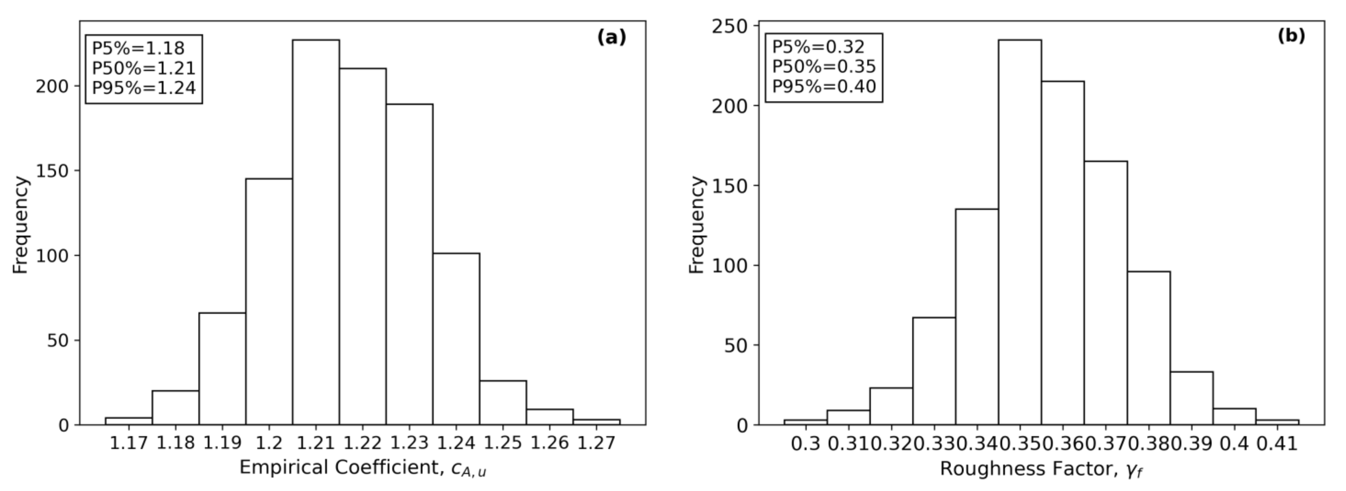The roughness factor, ${\gamma }_f$, obtained in this study using a two-level bootstrap resampling is not significantly different from that provided by EurOtop [2]. The optimum estimation in this study is determined using the 50% percentile of the roughness factor as ${\gamma }_f=$ 0.35. This value is slightly smaller than the roughness factor value by EurOtop [2], ${\gamma }_f=$ 0.38, for two-layered tetrapod armors. The similarity of the roughness factor values is likely due to both experiments with the same front slope ($V/H=$ 1/1.5). 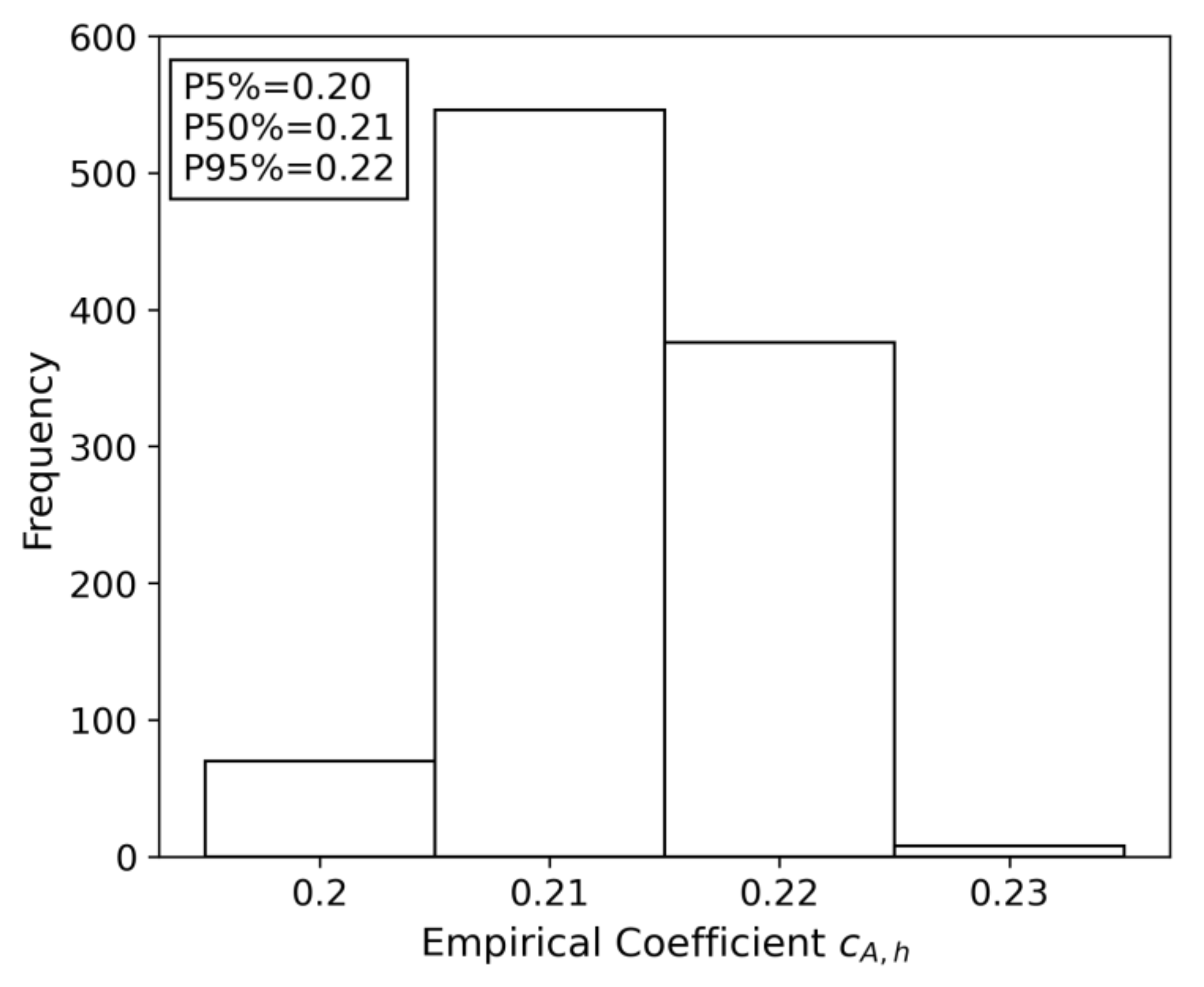The empirical coefficient, $c_{A,u}=1.21$, for the OFV in this study has a smaller value compared to $c_{A,u}=$ 1.30 from van Gent [5] conducting the reliable experiments. In the OLT, the optimum empirical coefficient, $c_{A,h}$, is determined using the 50% percentile as $c_{A,h}=$ 0.21. The $c_{A,h}$ value is close to $c_{A,h}=$ 0.20 by EurOtop [2]. The difference in the empirical coefficient for the OFV ($c_{A,u}$) is likely explained by the different structure geometry of the experiments, as discussed in Schüttrumpf and van Gent [15]. As shown in this study, using the empirical coefficients, $c_{A,u}$ and $c_{A,h}$, and roughness factor, ${\gamma }_f$, calibrated with the experiments can improve the estimation of OFV and OLT on composite breakwaters.

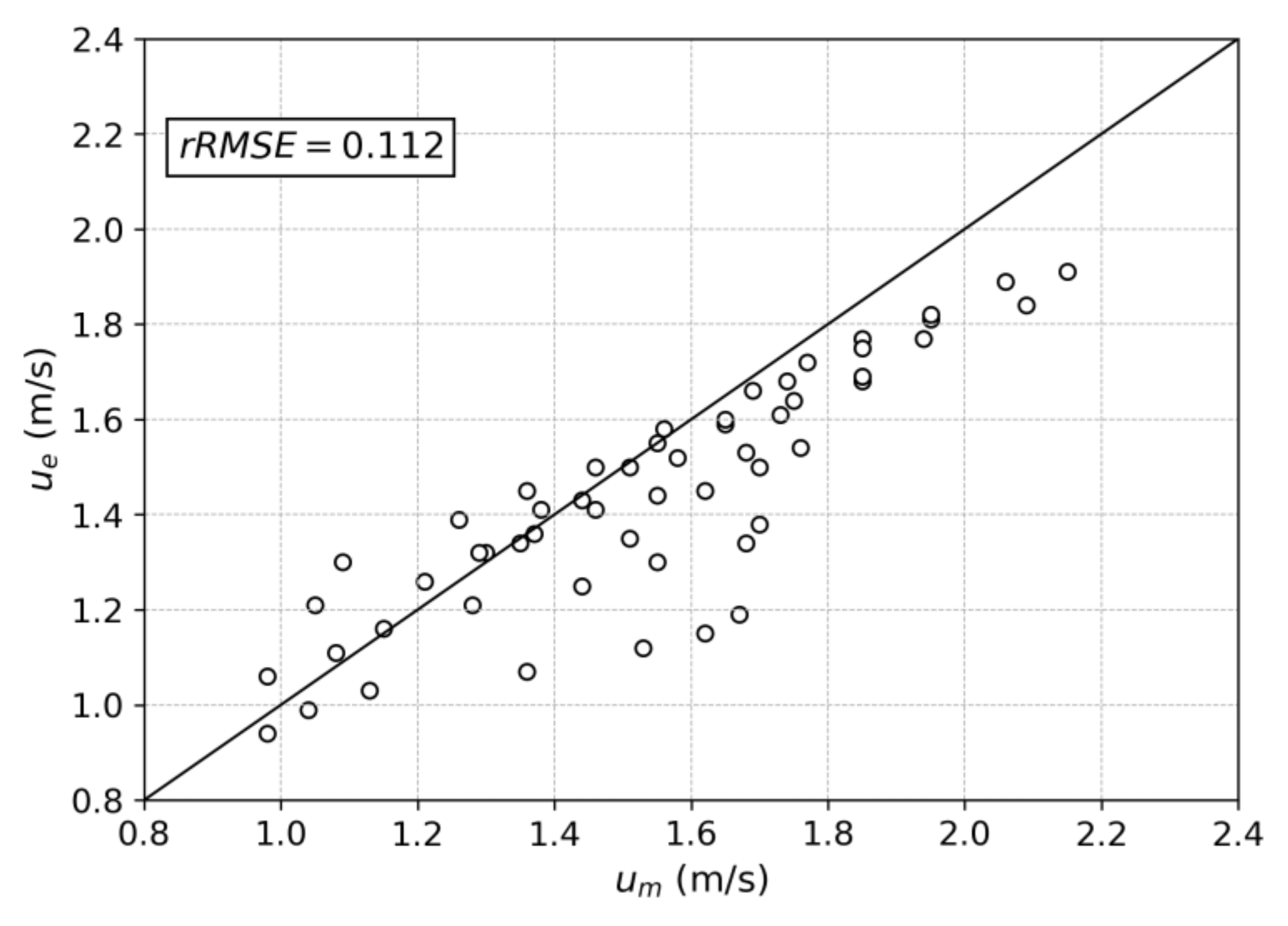
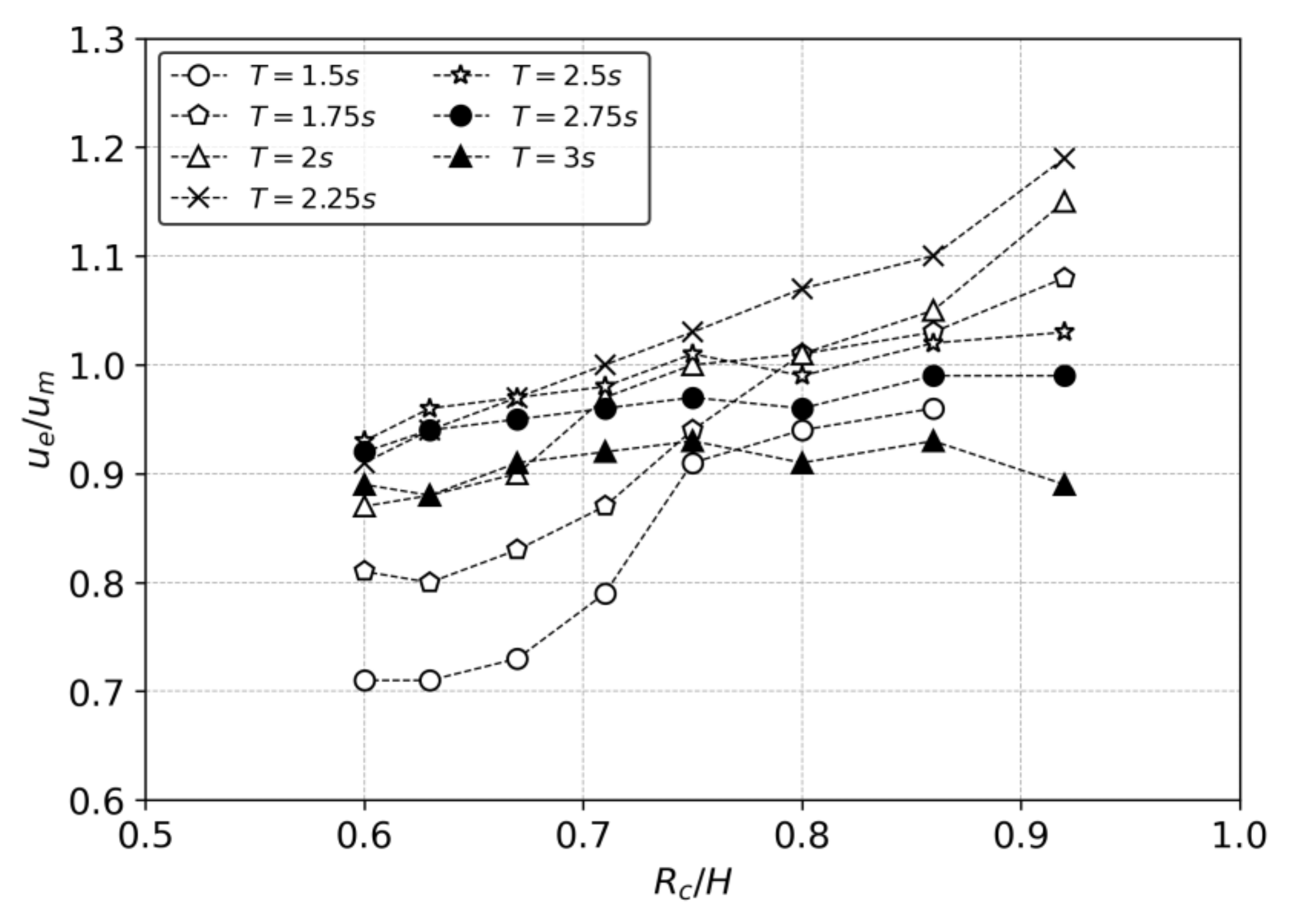
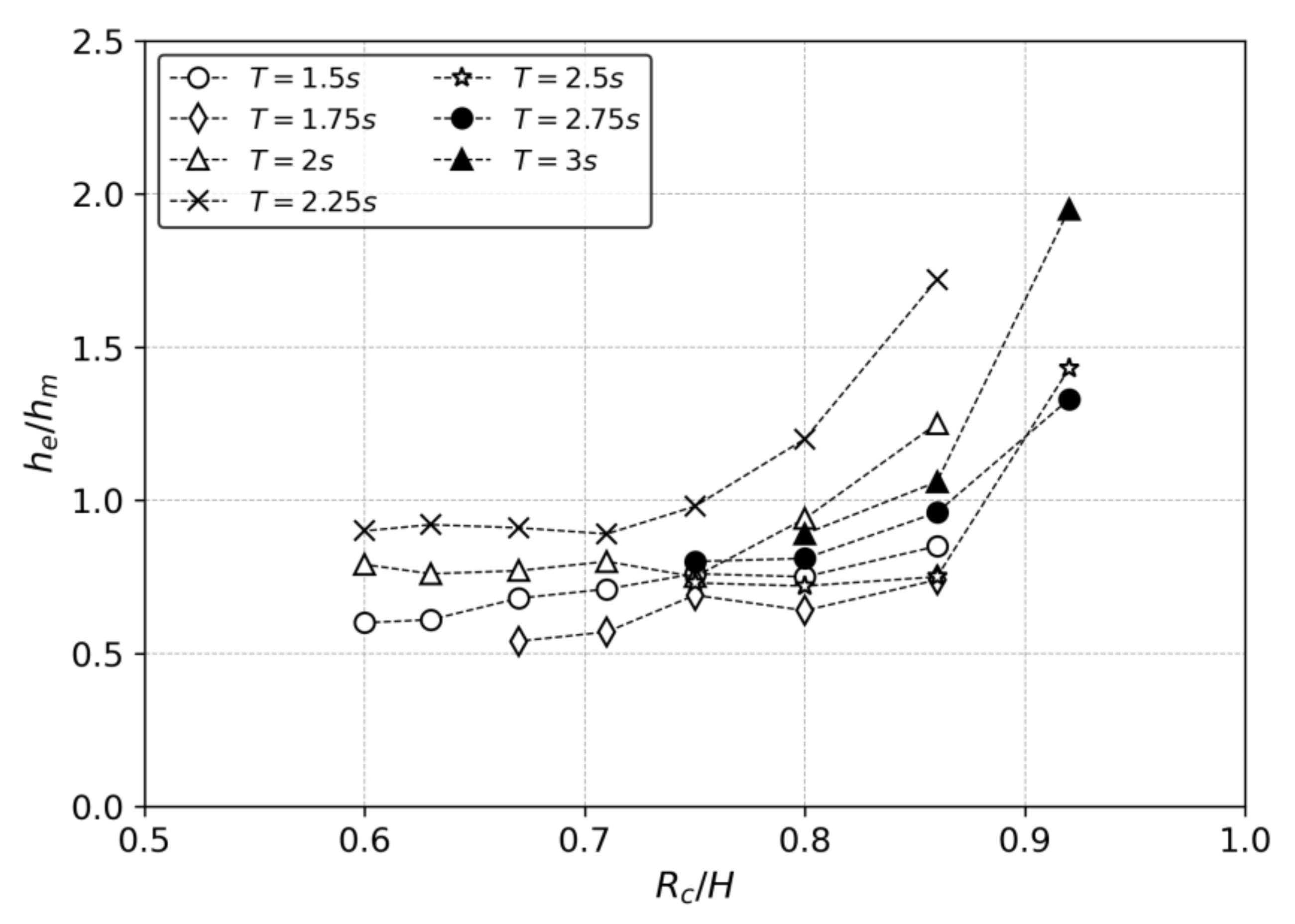
On the other hand, the estimated OFV, $u_e$, fluctuates in the wave period of $T=$ 1.5–2.25 s, where the $u_e$ is underestimated in the relatively large wave height and overestimated in the relatively small wave height. In the longer wave period of $T=$ 2.5–3.0 s, $u_e$ remains relatively constant. The patterns are likely explained by the different water wave conditions as presented in Table 2. 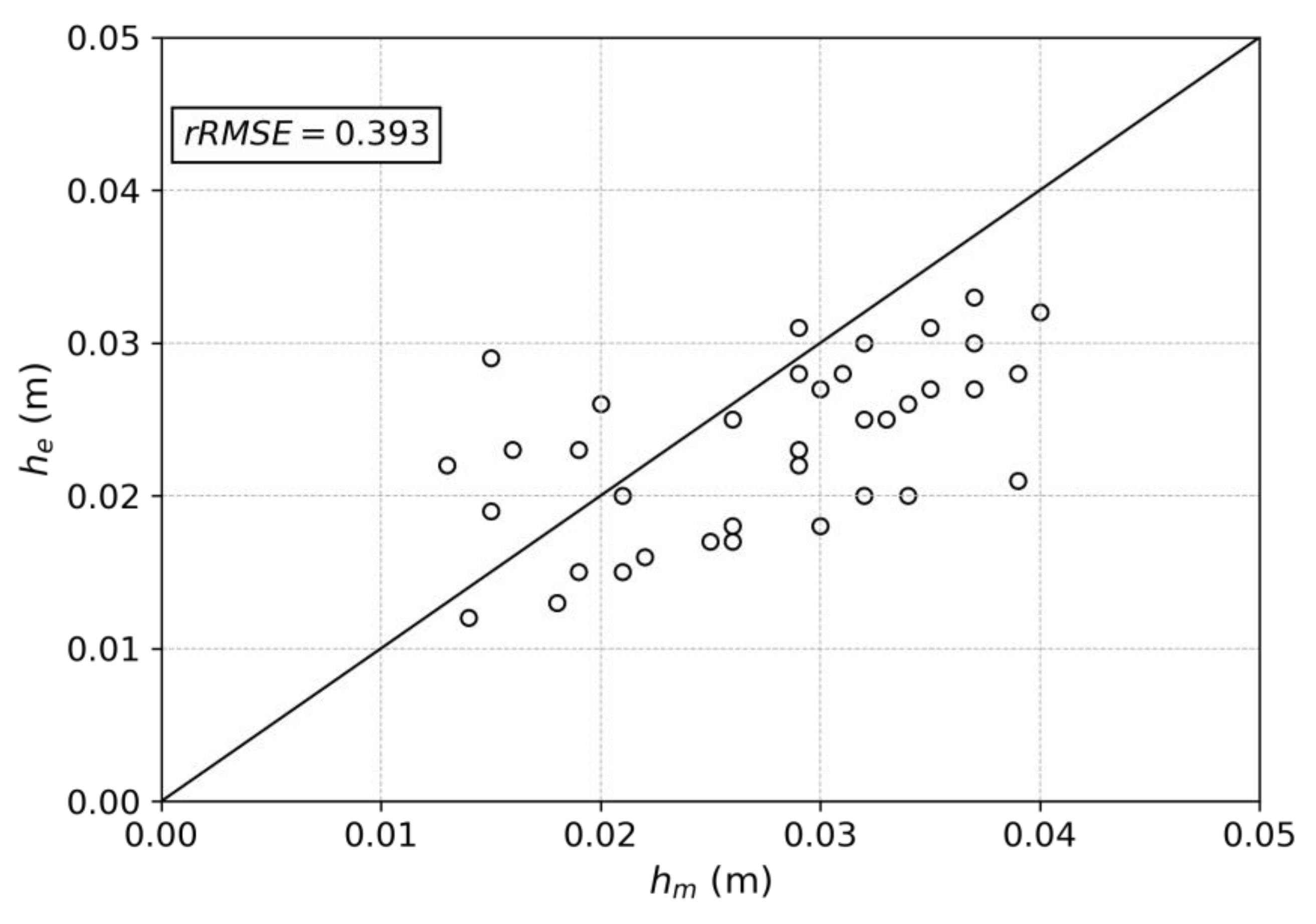Based on the linear wave theory, the shorter wave period used in this study is mostly of the intermediate water depth condition at the structure location (0.064 $< d/L <$ 0.114) and the longer wave period is close to the shallow water depth condition (0.028 $< d/L <$ 0.041). The overtopping flows of the short wave period are relatively sensitive to the interaction between the structure front and water waves, and are also subject to wave breaking as the wave height increases. The Iribarren’s number for the short wave period is in the range of 2.79–3.47, indicating the collapsing breaking type, which leads to wave breaking, causing nonlinearity and complicated interaction. In the OLT, a relatively uniform estimation is observed for the relatively large wave heights, but it mostly underestimates the OLT. As the wave height decreases, the estimated OLT ($h_e$) increases like the cases of OFV. Flows during the small wave heights are affected by most factors over the structure model and environmental conditions because the flows have relatively little momentum. The application of newly determined empirical coefficients shows the possibility of existing equations with optimized coefficients for various types of coastal structures. However, the discrepancy observed in relatively short and long waves means that a better empirical equation is needed to predict overtopping flows more accurately.

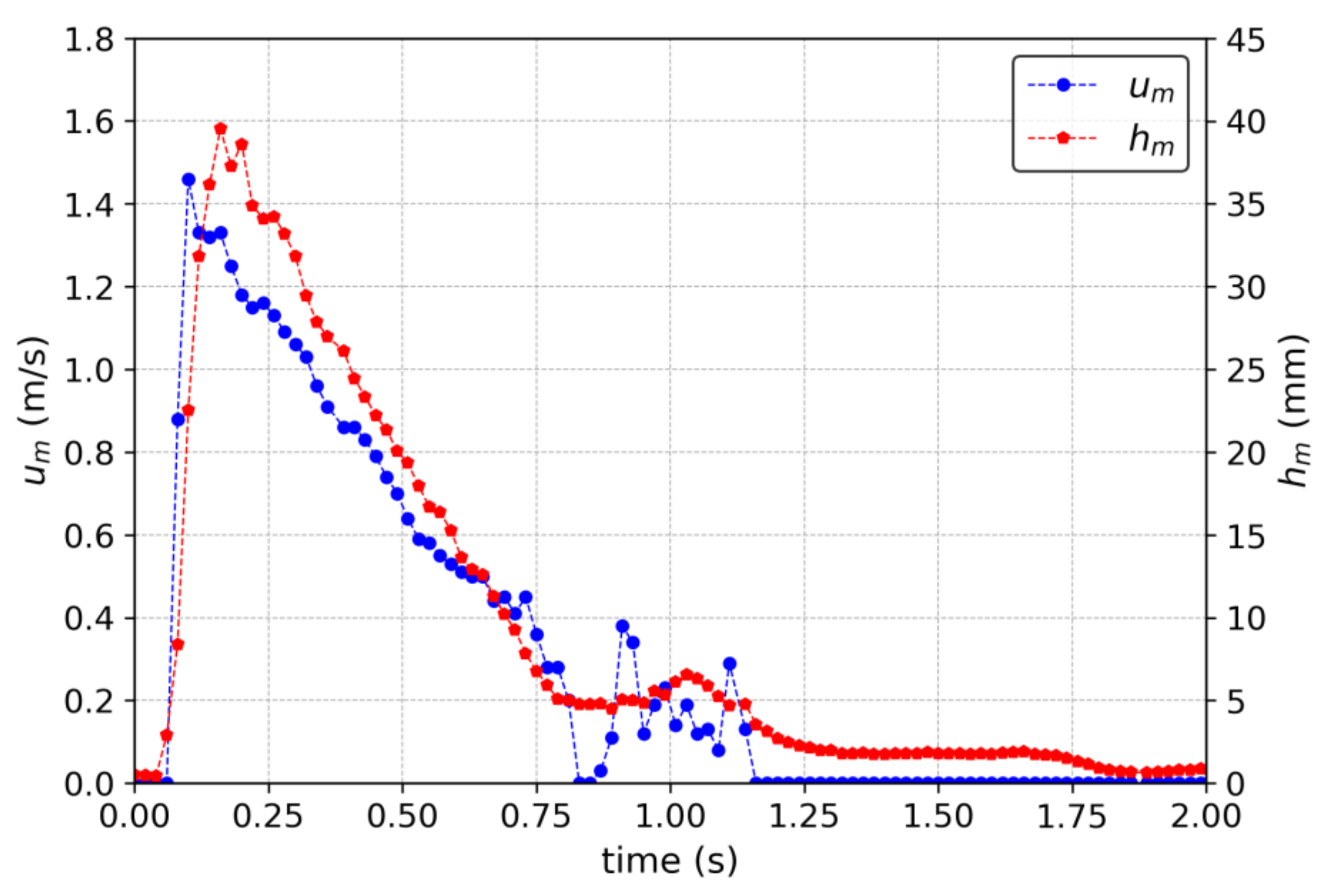
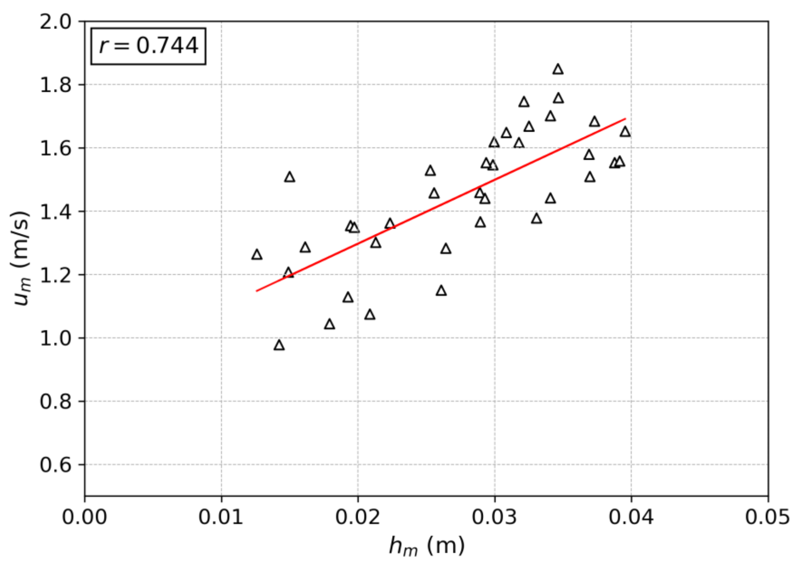
In this study, the OFV and OLT were measured from the same wave overtopping event. The maximum OFV occurred in the beginning stage first, and then the maximum OLT followed. There was little time difference between the maximum values, and they showed a similar temporal distribution pattern, which indicates the largest momentum of the flow occurs in the wavefront. From coupling OFV and OLT for the same event, there was a positive linear relationship between these two variables. This result differs from the result obtained by Mares-Nasarre et al. [10] and Hughes et al. [21], where there is no clear relationship between OFV and OLT. This difference may be due to the different methods used in the experiments. In this study, the spatial and temporal investigation using imaging techniques provided detailed information about the behavior of the overtopping flow properties, such as flow velocity and layer thickness. The OFV is determined from one of the vertically distributed horizontal velocity components, unlike the previous studies employing a point velocimeter. Moreover, the aeration of the overtopping flow is likely to lead to the inaccurate acquisition of the free surface by a capacitance-type wave gauge. From the flow images, the aeration was observed in the wave front where the max OLT occurred, which implies the possibility of errors in catching maximum values. From the positive relationship between OFV and OLT in this study, the rapidly increasing rate of momentum is expected relative to OFV and OLT.

6. Conclusions

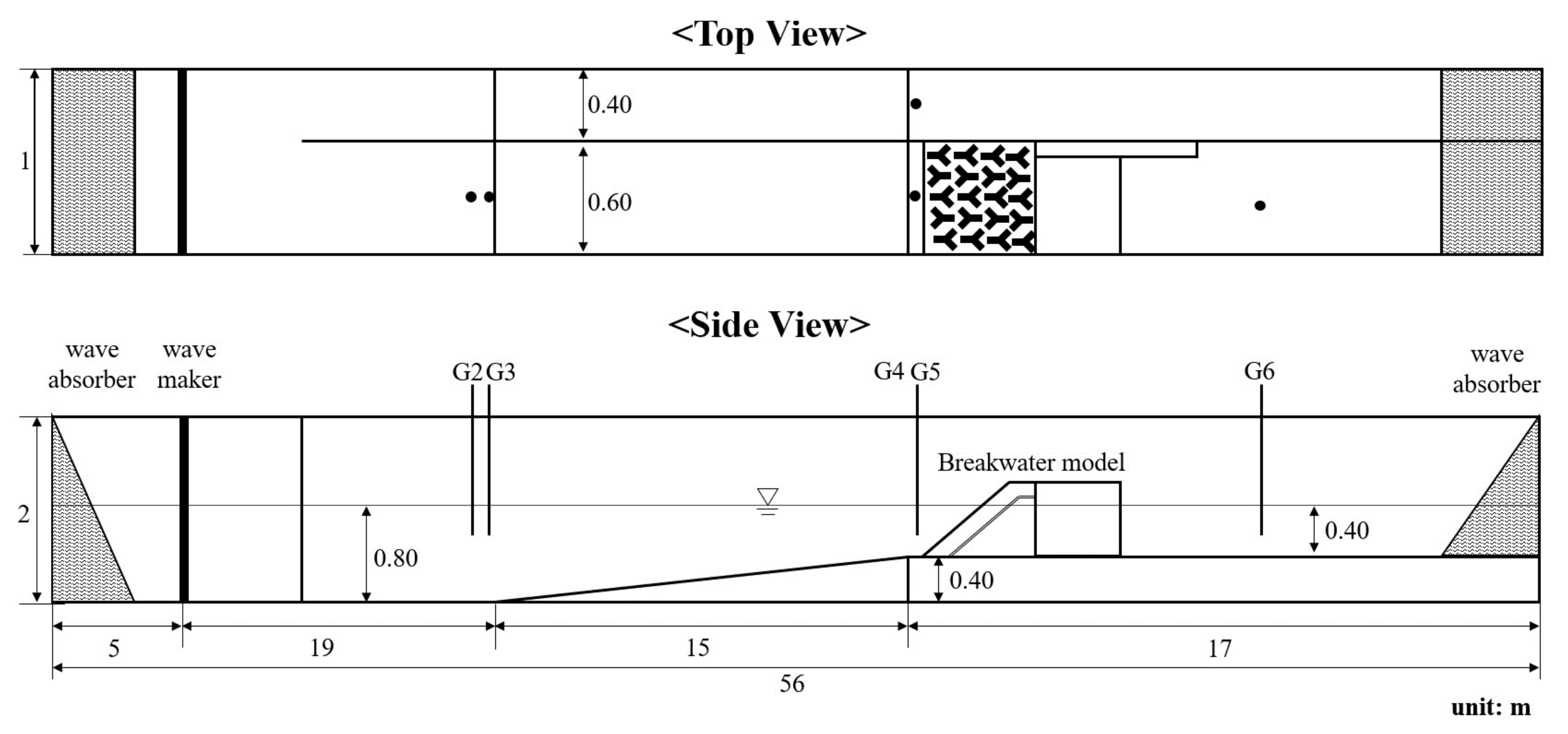
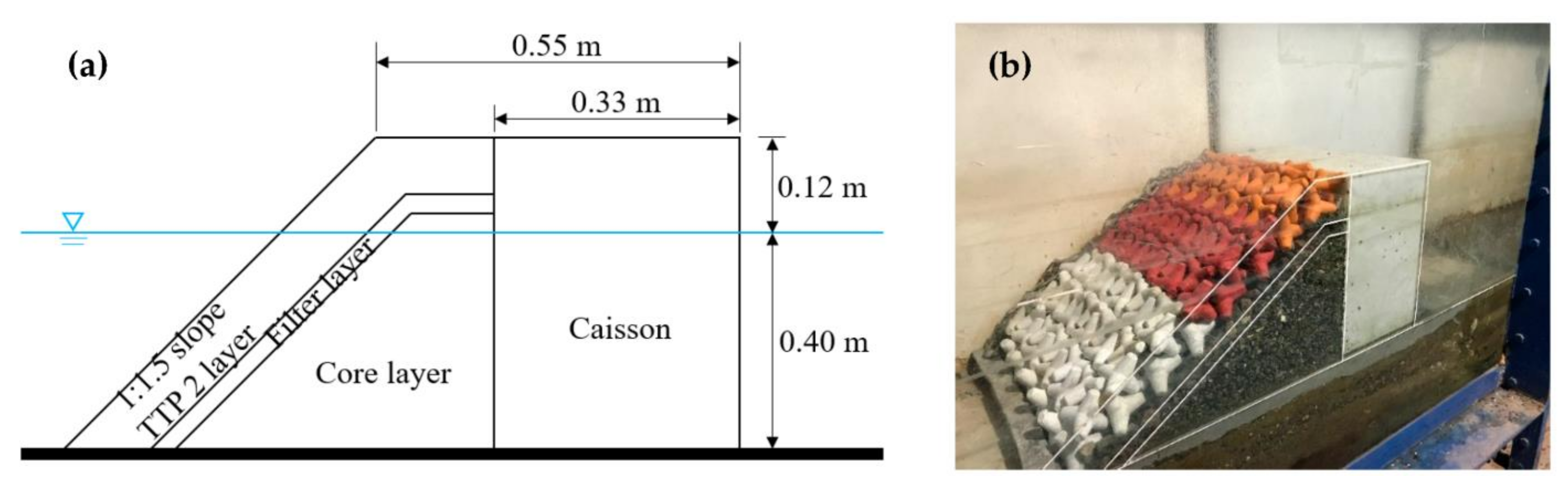
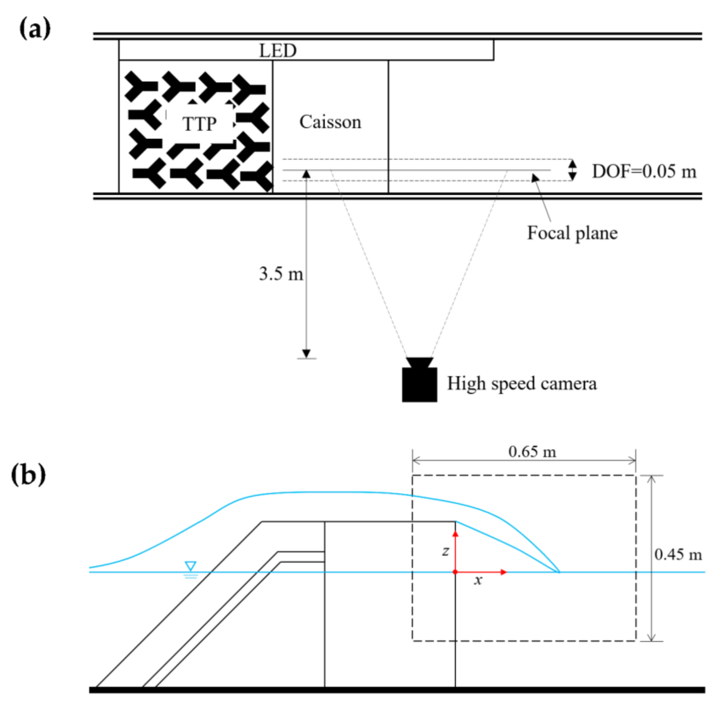
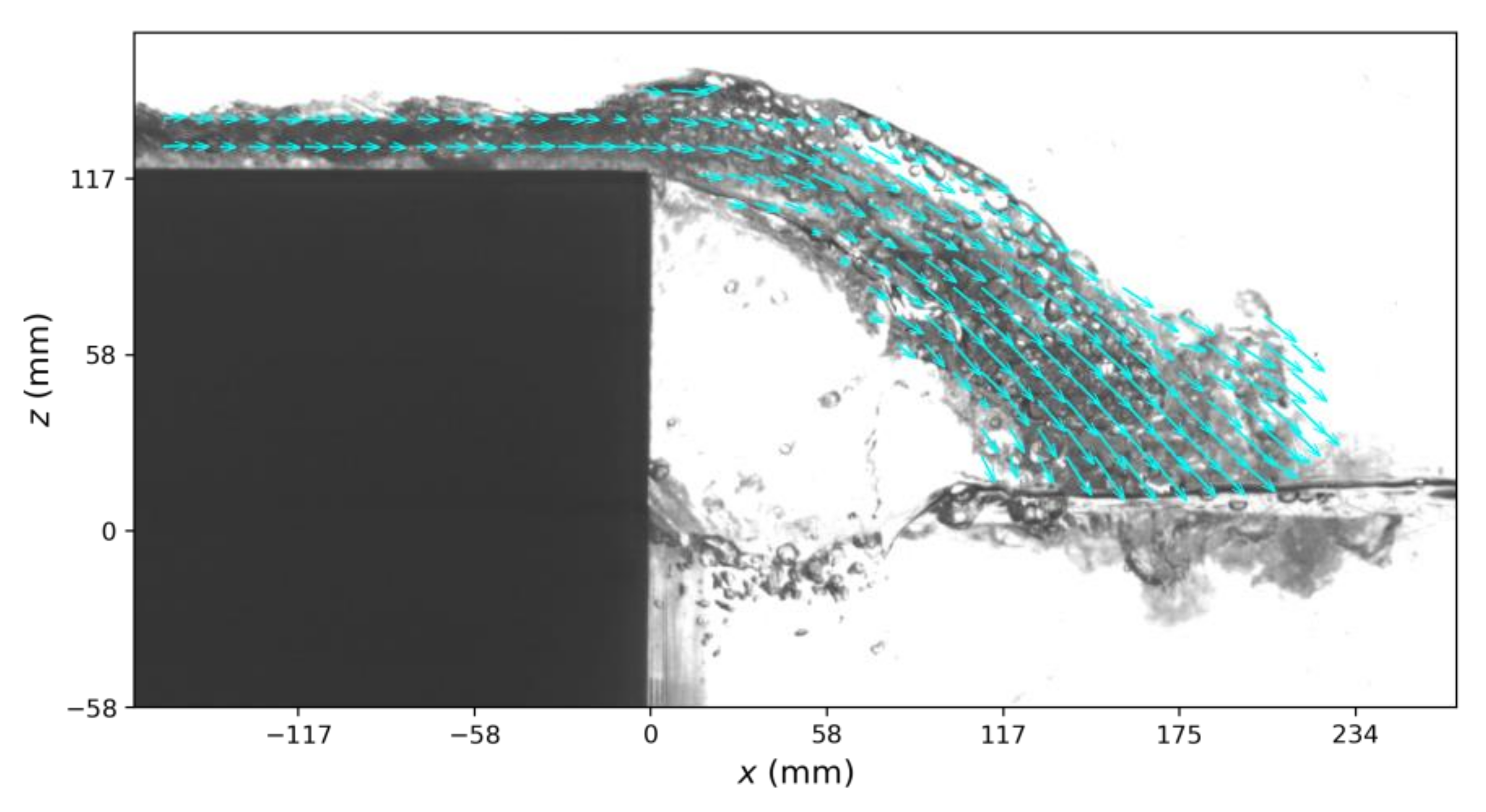
The wave overtopping occurs when the wave run-up, $R_u$, is higher than the crest freeboard of a coastal structure, $R_c$. In such conditions, the water wave affects not only the structure’s front slope but also the structure’s crest and rear side. In addition, wave overtopping also poses a threat to the safety of people and vehicles on the structure crest. However, most of the previous studies have focused on wave overtopping flow parameters on impermeable structures such as sea dikes, with only a few studies on breakwaters. To address this gap, this study investigated OFV and OLT on composite breakwaters through physical experimentation. In this study, 55 physical tests for the composite breakwater with the tetrapod armors were performed on the two-dimensional wave flume. The OFV at the rear edge of the breakwater crest was measured using a digital imaging technique called bubble image velocimetry (BIV), which provides reliable measurements without disturbing the overtopping flow. The OLT was measured by digitizing the digital images obtained from the BIV technique.

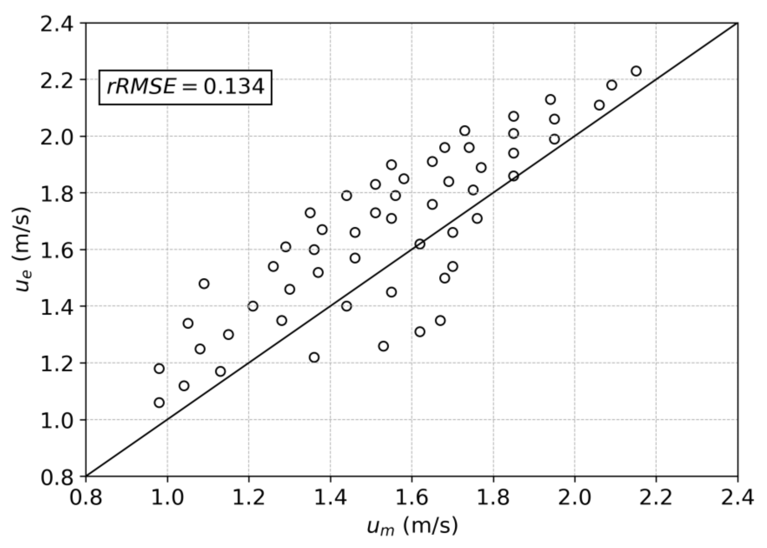
The measured OFV and OLT were compared with the empirical equations provided in EurOtop [2], Schüttrumpf and van Gent [15], and van der Meer et al. [7]. The roughness factor, ${\gamma }_f$, in Equation (12) and the empirical coefficients, $c_{A,u}$ and $c_{A,h}$, in Equations (5) and (6) were calibrated with the experiment data. The new roughness factor for the two-layered tetrapods, ${\gamma }_f=$ 0.35, and empirical coefficients, $c_{A,u}=$ 1.21 and $c_{A,h}=$ 0.21, were obtained through the bootstrap resampling technique. The rRMSE for the estimation of OFV was 0.112 and that of the OLT was 0.393. The new empirical coefficients and roughness factor obtained in this study were used to estimate the OFV and OLT in various wave conditions, which shows promising results for relevant coefficient determination. However, the agreements between the estimations and the measurements are not consistent over all wave conditions and structure geometries. In particular, the estimation for short-wave conditions showing discrepancies needs to be approached through another empirical formula. The results of this study are applicable to composite breakwater structures with armor slope $V/H=$ 1:1.5 and relative crest freeboard 0.6 $< R_c/H <$ 1 in non-breaking wave condition 0.008 $< H/L_o <$ 0.057. More advanced empirical approaches are needed and will be further tested for irregular wave conditions as well.

From the temporal change of OFV and OLT, both parameters show the maximum values with little time difference in the wavefront, having a pattern of sudden increase and gradual decrease. Therefore, the largest momentum of the overtopping flow is expected to occur in the beginning stage of the flow. There is also a positive relationship between OFV and OLT for the same overtopping event, which implies that the momentum of the flow and overtopping volume would increase rapidly.

References

1. Argente, G.; Gómez-Martín, M.E.; Medina, J.R. Hydraulic Stability of the Armor Layer of Overtopped Breakwaters. J. Mar. Sci. Eng. 2018, 6, 143. [Google Scholar] [CrossRef] [Green Version]
2. Van der Meer, J.W.; Allsop, N.W.H.; Bruce, T.; De Rouck, J.; Kortenhaus, A.; Pullen, T.; Schüttrumpf, H.; Troch, P.; Zanuttigh, B. EurOtop-Manual on Wave Overtopping of Sea Defences and Related Structures: An Overtopping Manual Largely Based on European Research, but for Worldwide Application; TU Delft: Delft, The Netherlands, 2018. [Google Scholar]
3. Gao, J.; Ma, X.; Zang, J.; Dong, G.; Ma, X.; Zhu, Y.; Zhou, L. Numerical Investigation of Harbor Oscillations Induced by Focused Transient Wave Groups. Coast. Eng. 2020, 158, 103670. [Google Scholar] [CrossRef]
4. Gao, J.; Ma, X.; Dong, G.; Chen, H.; Liu, Q.; Zang, J. Investigation on the Effects of Bragg Reflection on Harbor Oscillations. Coast. Eng. 2021, 170, 103977. [Google Scholar] [CrossRef]
5. Van Gent, M.R.A. Wave Overtopping Events at Dikes. In Coastal Engineering 2002; World Scientific: Singapore, 2002; pp. 2203–2215. ISBN 978-981-238-238-2. [Google Scholar]
6. Schüttrumpf, H.; Möller, J.; Oumeraci, H. Overtopping Flow Parameters on The Inner Slope of Seadikes. In Coastal Engineering 2002; World Scientific Publishing Company: Singapore, 2002; pp. 2116–2127. [Google Scholar]
7. Van der Meer, J.W.; Hardeman, B.; Steendam, G.J.; Schuttrumpf, H.; Verheij, H. Flow Depths and Velocities at Crest and Landward Slope of a Dike, in Theory and with The Wave Overtopping Simulator. Coast. Eng. Proc. 2011, 1, structures.10. [Google Scholar] [CrossRef] [Green Version]
8. Bae, H.U.; Yun, K.M.; Yoon, J.Y.; Lim, N.H. Human Stability with Respect to Overtopping Flow on the Breakwater. Int. J. Appl. Eng. Res. 2016, 11, 111–119. [Google Scholar]
9. Cao, D.; Yuan, J.; Chen, H.; Zhao, K.; Liu, P.L.-F. Wave Overtopping Flow Striking a Human Body on the Crest of an Impermeable Sloped Seawall. Part I: Physical Modeling. Coast. Eng. 2021, 167, 103891. [Google Scholar] [CrossRef]
10. Mares-Nasarre, P.; Argente, G.; Gómez-Martín, M.E.; Medina, J.R. Overtopping Layer Thickness and Overtopping Flow Velocity on Mound Breakwaters. Coast. Eng. 2019, 154, 103561. [Google Scholar] [CrossRef]
11. Mares-Nasarre, P.; Gómez-Martín, M.E.; Medina, J.R. Influence of Mild Bottom Slopes on the Overtopping Flow over Mound Breakwaters under Depth-Limited Breaking Wave Conditions. J. Mar. Sci. Eng. 2020, 8, 3. [Google Scholar] [CrossRef] [Green Version]
12. Mares-Nasarre, P.; Molines, J.; Gómez-Martín, M.E.; Medina, J.R. Explicit Neural Network-Derived Formula for Overtopping Flow on Mound Breakwaters in Depth-Limited Breaking Wave Conditions. Coast. Eng. 2021, 164, 103810. [Google Scholar] [CrossRef]
13. Molines, J.; Medina, J.R. Calibration of Overtopping Roughness Factors for Concrete Armor Units in Non-Breaking Conditions Using the CLASH Database. Coast. Eng. 2015, 96, 62–70. [Google Scholar] [CrossRef] [Green Version]
14. Pepi, Y.; Romano, A.; Franco, L. Wave Overtopping at Rubble Mound Breakwaters: A New Method to Estimate Roughness Factor for Rock Armours under Non-Breaking Waves. Coast. Eng. 2022, 178, 104197. [Google Scholar] [CrossRef]
15. Schüttrumpf, H.; van Gent, M.R.A. Wave Overtopping at Seadikes. In Coastal Structures 2003; American Society of Civil Engineers: Reston, VA, USA, 2003; pp. 431–443. [Google Scholar]
16. Van Gent, M.R.A. Wave Runup on Dikes with Shallow Foreshores. J. Waterw. Port Coast. Ocean Eng. 2001, 127, 254–262. [Google Scholar] [CrossRef]
17. Bosman, G.; van der Meer, J.; Hoffmans, G.; Schüttrumpf, H.; Verhagen, H.J. Individual Overtopping Events at Dikes. In Coastal Engineering 2008; World Scientific: Singapore, 2009; pp. 2944–2956. [Google Scholar] [CrossRef] [Green Version]
18. Lorke, S.; Scheres, B.; Schuttrumpf, H.; Bornschein, A.; Pohl, R. Physical Model Tests on Wave Overtopping and Flow Processes on Dike Crests Influenced by Wave-Current Interaction. Coast. Eng. Proc. 2012, 1, waves.34. [Google Scholar] [CrossRef] [Green Version]
19. Ryu, Y.; Chang, K.-A.; Lim, H.-J. Use of Bubble Image Velocimetry for Measurement of Plunging Wave Impinging on Structure and Associated Greenwater. Meas. Sci. Technol. 2005, 16, 1945. [Google Scholar] [CrossRef]
20. Thielicke, W.; Stamhuis, E.J. PIVlab—Towards User-Friendly, Affordable and Accurate Digital Particle Image Velocimetry in MATLAB. J. Open Res. Softw. 2014, 2, 30. [Google Scholar] [CrossRef] [Green Version]
21. Hughes, S.A.; Thornton, C.I.; Van der Meer, J.W.; Scholl, B.N. Improvements in Describing Wave Overtopping Processes. Coast. Eng. Proc. 2012, 1, waves.35. [Google Scholar] [CrossRef]
Figure 1. Definition sketch of fictitious wave run-up (a) and wave overtopping (b). The wave run-up and wave overtopping parameters are based on Schüttrumpf and van Gent [15].
Jmse 11 00823 g001
Figure 2. Dimensions of the wave flume.
Jmse 11 00823 g002
Figure 3. Composite breakwater model: (a) the sketch of the breakwater model and (b) the picture of the breakwater.
Jmse 11 00823 g003
Figure 4. Scheme of the BIV setup: (a) Camera position and (b) the field of view (FOV).
Jmse 11 00823 g004
Figure 5. Snapshot of the velocity map of wave overtopping flow plunging on the rear side of the breakwater.
Jmse 11 00823 g005
Figure 6. OFV ( u m ) and OLT ( h m ) at the rear edge breakwater crest. The wave condition was T = 2.75 s and H = 16 cm.
Jmse 11 00823 g006
Figure 7. Comparisons of the measured and estimated OFV for c A , u = 1.3 and γ f = 0.38 with rRMSE = 0.134 and R 2 = 0.702.
Jmse 11 00823 g007
Figure 8. Histogram plot of the empirical coefficient, c A , u , and the roughness factor, γ f , obtained from the bootstrap resampling: (a) the first level bootstrap and (b) the second level bootstrap.
Jmse 11 00823 g008
Figure 9. Comparison of the measured OFV and the estimation using c A , u = 1.21 and γ f = 0.35.
Jmse 11 00823 g009
Figure 10. Estimation of the OFV relative to the measurements in the different wave conditions.
Jmse 11 00823 g010
Figure 11. Histogram of the empirical coefficient, c A , h , obtained from the bootstrap resampling.
Jmse 11 00823 g011
Figure 12. Comparison between the measured and estimated OLT.
Jmse 11 00823 g012
Figure 13. Estimation of the OLT relative to the measurements in the different wave conditions.
Jmse 11 00823 g013
Figure 14. Comparison of the measured OFV and OLT at the rear edge breakwater crest corresponding to the same wave overtopping event.
Jmse 11 00823 g014