Enhancement of the Robustness on Advancing Layer Method with Trimmed Hexahedral Volume Mesh for the Generation of the Boundary Layer Grids

Abstract

When performing simulations using computational fluid dynamics, the grid systems in the viscous boundary layer regions are important because the velocity and pressure change very rapidly in these regions. Especially for the turbulent flows, thin grids should be arranged densely in the direction perpendicular to the wall. In this study, the advancing layer method, which has been applied mostly to tetrahedral meshes, is applied to trimmed hexahedral meshes. To generate boundary layer meshes with non-intersecting grid lines near the wall boundaries having concave corners and narrow gaps, the directional vectors of grid lines and faces are smoothed, and the displacement vector fields calculated using the Laplace equation were utilized. Firstly, the details on the newly developed methods are introduced showing simple two-dimensional cases as examples. After applying the methods for a complex three-dimensional geometry to check its applicability and investigating the generated grid systems, the numerical simulations of propeller open water test for INSEAN E779A marine propeller were carried out by simpleFoam, one of the standard solvers of OpenFOAM. The computational results showed good agreement with the experimental results. Therefore, in conclusion, the developed advancing layer method is an appropriate method for generating boundary layer grids of a trimmed hexahedral mesh.

1. Introduction

The recent major issues in the Korean shipbuilding and maritime industry are environmental, social, governance (ESG) management, and digital transformation (DX); in particular, DX has been highly promoted as a breakthrough that can overcome the overall industrial downturn and enhance global competitiveness. DX can be largely classified into digital, management, engineering, manufacturing, product, platform, and culture, and computer-aided engineering (CAE) is one of the core components. CAE, such as computational fluid dynamics (CFD), finite element analysis, and multi-physics simulation using computers, has attracted a great deal of attention and is widely used in various fields of academia, research, and industry due to the rapid progression in computational performance and technology.

For CFD simulations, grid systems are generally used in the Eulerian frames for both the structured grids [1], unstructured grids [2], and solvers compatible with the adopted grids. Recently, unstructured grids and solvers that use the finite volume method (FVM) [3] have been largely applied to discretize the governing equations owing to their ease of representing complex objects despite their relatively lower accuracy and higher computational costs compared with those of structured ones. Unlike the grid-based method, which must maintain connection information with adjacent grids, the gridless method, which is also referred to as meshless or mesh-free, requires only the location information and physical quantities of computational points for spatial differential approximation at the points [4].

When utilizing CFD for the simulations of viscous flows facing wall boundaries, proper arrangement of computational points and grid systems near the boundaries are one of the most important factors to ensure the accuracy and stability of the simulations, whether it is based on grid or gridless methods. In the case of grid-based methods, grids should be composed of grid lines parallel and normal to the wall boundary, in principle, because the velocity and pressure in the boundary layer regions change very rapidly. Especially for the turbulent flows, thin grids should be arranged densely in the direction perpendicular to the wall. However, if a three-dimensional (3-D) body with a complex geometry exists inside the fluid domain or the shape of the bounding wall boundaries are complex, the generation of proper boundary layer grids are difficult. Concave edges and/or narrow gaps makes the generation more difficult. Therefore, many researchers have invested considerable effort in developing fast, efficient, and automatic methods for generating volume meshes with boundary layers grids.

Generally, methods based on tetrahedral mesh and octree-based Cartesian meshes are used to generate unstructured volume meshes for the problem including 3-D complex geometries. A tetrahedral mesh accurately implements complex shapes, and three-dimensional advancing front method [5] and Delaunay-based [6,7] tetrahedral meshes are widely used. However, because the grid is isotropic, these methods are suitable for inviscid flow simulations. Therefore, it needs to adopt a method of generating anisotropic meshes or hybrid meshes around the walls for viscous flows. Although cartesian mesh is fast, it is difficult to precisely represent the shape. To solve this problem, methods such as the cut-cell method [8], building-cube method [9], and immersed boundary method [10] have been proposed. Recently, a trimmed hexahedral mesh method based on a cartesian cut-cell has also been developed [11,12].

To generate boundary layer grids, the advancing layer method was proposed by Zhi and Jaime [13]. In their research, the whole-layer inflation method and the layer-by-layer approach were introduced. The merits of the former method are the robustness and quality adopting partial generation of boundary grids, that is, the boundary layer continues to be stacked where the grid can be stacked but not stacked in difficult regions. In the latter case, whole-layer inflation method has an advantage over the very fast generation speed. However, the thickness of the boundary layer grids becomes significantly thin in a narrow region, which can deteriorate the shape of the volume mesh, and the volume ratio becomes very large because the same number of boundary layers are forced to be stacked around the all the wall boundaries.

Methods of generating the boundary layer grids can be divided into the open advancing layer method, which inflates the wall grid to create the boundary layer grids and then creates the volume grid, and the closed advancing layer method, which first creates the volume grid and then inflates the boundary layer grids [13,14]. In their studies, it was said that the advantage of the closed advancing layer method is that it always ensures that grids are valid because it departs from a valid volumetric mesh. However, it is also noted that an effective, efficient, and robust volumetric mesh deformation algorithm is the key to achieving high quality meshes, especially when dealing with highly complex geometries. In [14], grid optimization was performed at each stage while inflating in a layer-by-layer method. In addition, three calculating methods for normal vectors and the comparisons of the grids generated by these methods were introduced because the normal vectors at vertices play a fundamental role in boundary layer meshing, as the mesh is extruded from the surface triangulation along the point normal vectors.

To summarize, most of the developed methods are based on the tetrahedral volume meshes and there still have been difficulties generating boundary layer grids for especially turbulent, viscous flow simulations. Moreover, the importance of the volume mesh deformation and normal vectors were pointed out.

In the present study, the advancing layer method is applied to the trimmed hexahedral meshes generated by the previously developed cut-cell method [11]. To generate boundary layer meshes with grid lines that are not intersected near the wall boundaries where concave corners and narrow gaps exist, the directional vectors of grid lines and faces are smoothed, and the displacement vector fields calculated using the Laplace equation were utilized. The details of the newly developed method are introduced by considering a simple two-dimensional (2-D) case as an example first. After applying the method to complex three-dimensional geometries to check its applicability and investigate the generated grid system, numerical simulations of the propeller open water (POW) test for a marine propeller were performed using one of the standard solvers of OpenFOAM. The reason for choosing the POW test as for the validation is that the marine propeller has complex shape, and its efficiency is highly significant because it directly affects the propulsion performance of a marine vessel.

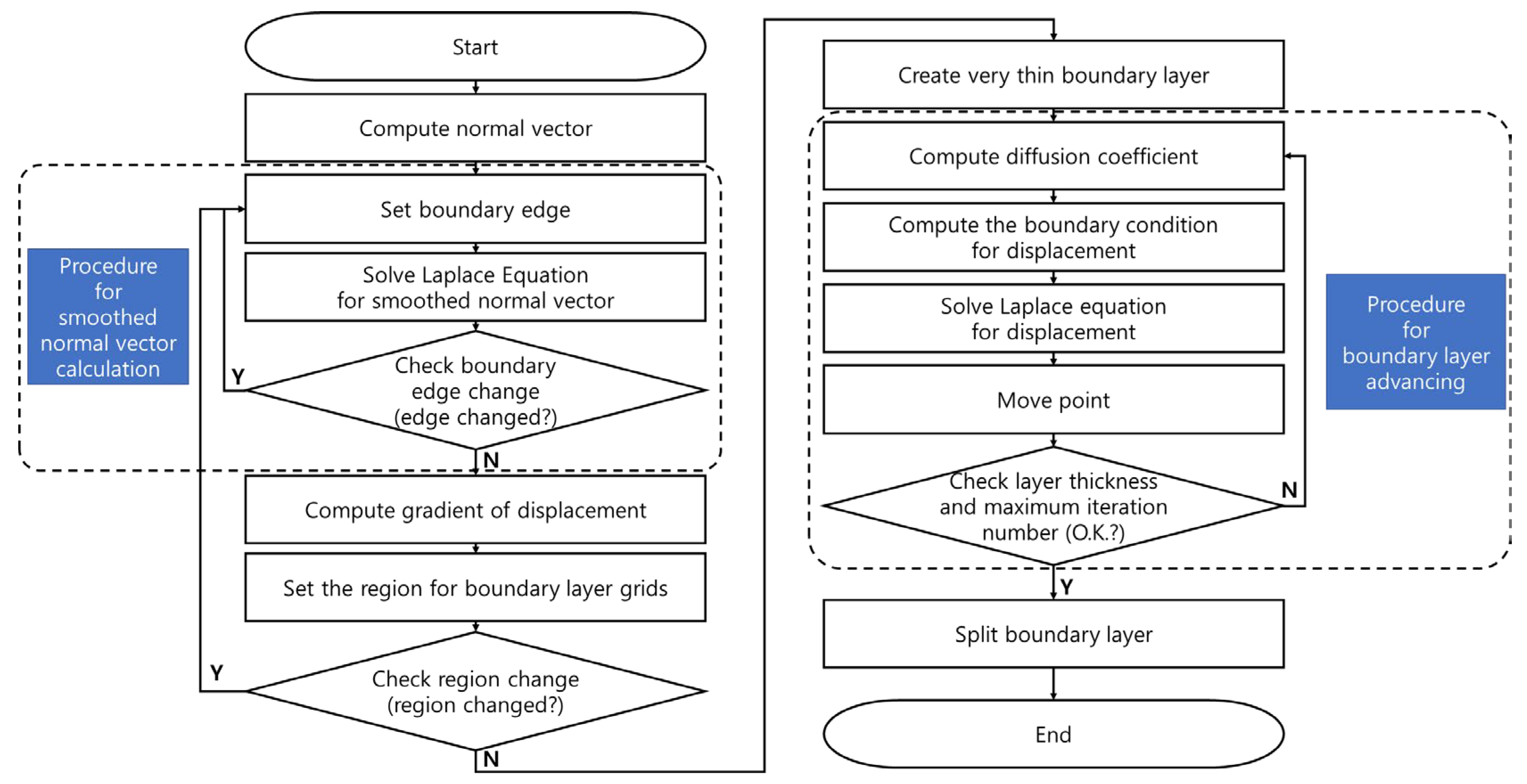
2. Numerical Methods

In this chapter, the newly developed advancing layer method is introduced. The main target of the method is to generate boundary layer meshes with grid lines that are not intersected near the wall boundaries where concave corners and narrow gaps exist. Fully polyhedral meshes based on the locally anisotropic (2N-tree) refined cut-cell method, which was developed by Jeong and Seo [11], were used for the base volume meshes.

The overall procedure for the boundary layer grid generation is shown in Figure 1 and summarized as follows:

• Calculating normal vectors of boundary faces,
• Calculating smoothed normal vector and displacement vector,
• Searching for the regions where boundary layer grids cannot be generated,
• Recalculating smoothed normal vector and displacement vector,
• Creating very thin boundary layer grids by copying corresponding boundary grids,
• Creating a boundary layer grid by moving the copied grid points while gradually increasing the displacement vector,
• Cutting and finalizing the boundary layer grids.

Figure 1. Flow chart for boundary layer generation.

Figure 1. Flow chart for boundary layer generation.

Hereafter, the main algorithms of the developed method are introduced with the simplified notation of ‘normal vector’ instead of ‘unit normal vector’.

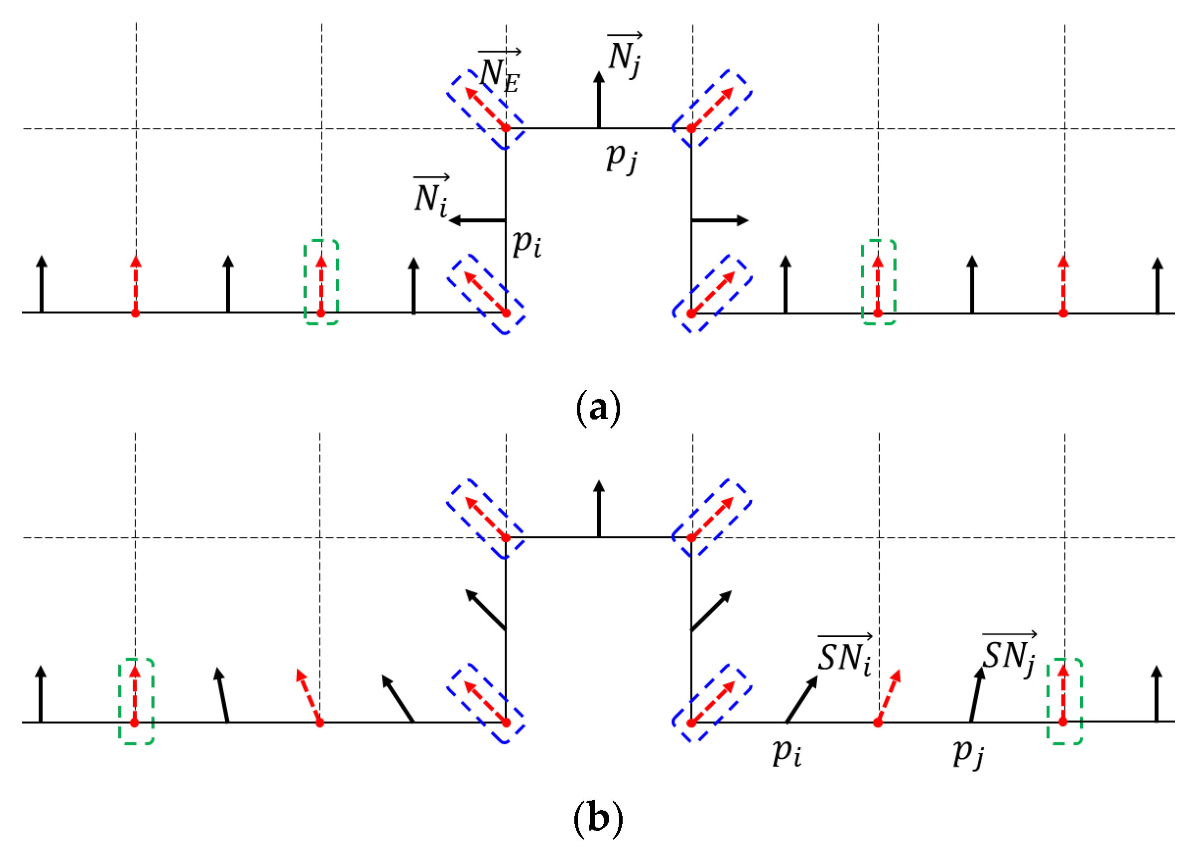
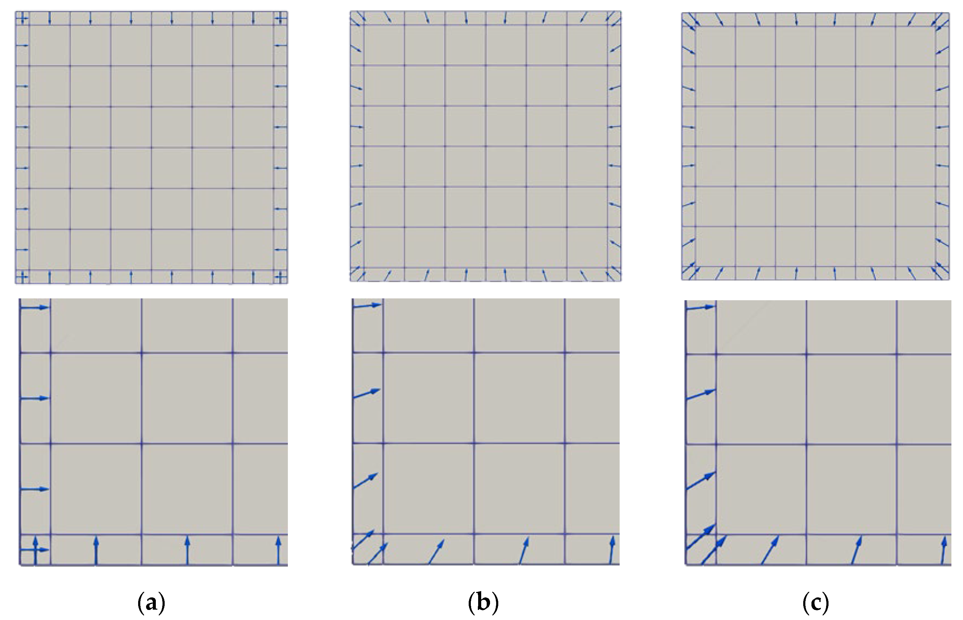
2.1. Advancing Direction Calculation

Solving the Laplace equation using surface normal vectors as its boundary conditions is one of the well-known and typical grid generation methods for the body-fitted tetrahedral grids [14,15] and boundary layer grids. However, evidently, boundary layer grids are not generated at the concave edges, such as the corners of a rectangular, by calculating the distributions of displacement and moving the grids using the Laplace equation. The reason for this problem is that the boundary conditions of each boundary face constrain the tangential displacement of the boundary grid lines. To solve such type of problems, a method to smooth the normal vector at the concave edges is developed and applied in this study.

To get the smoothed normal vectors of boundary grid line and faces, the Laplace equation in Equation (1) is iteratively solved.

$$\nabla ·(\Gamma \nabla \overrightarrow{D})=0,$$

(1)

where $\Gamma$ is the constant diffusion coefficient, and $\overrightarrow{D}$ is the smoothed normal vector $\overrightarrow{SN}$ or displacement vector $\overrightarrow{D_b}$. The normal vector of the grid line $\overrightarrow{N_E}$ is calculated by Equation (2) and used as the boundary condition in the Equation (1)

$$\overrightarrow{N_E}=\frac{(\overrightarrow{N_i}+\overrightarrow{N_j})}{\mid (\overrightarrow{N_i}+\overrightarrow{N_j})\mid },$$

(2)

where $\overrightarrow{N_i}$ and $\overrightarrow{N_j}$ are the normal vectors of the neighboring grid faces.

An example of $\overrightarrow{N_E}$, $\overrightarrow{N_i}$, and $\overrightarrow{N_j}$ can be found in Figure 2a, where the black and red arrows represent the normal vectors of boundary grid face and boundary grid line, respectively. In the figure, the start point of $\overrightarrow{N_E}$ is the point or edge in 2-D and 3-D spaces, respectively, where two boundary grid lines share a point or edge. For the boundary condition of the Laplace equation, normal vectors inside the dashed boxes were used.

The point or edge, where the intersecting angle between the normal vectors of the neighboring boundary grid faces is significantly large, is set as and used for the boundary condition for the Laplace equation, as marked by the blue dashed box in Figure 2. The purpose for this treatment is to prevent the difference between the initial and smoothed normal vectors from becoming excessively large. In the present study, Equation (3) is used to judge whether the intersecting angle is large.

$$if \overrightarrow{N_i}·\overrightarrow{N_j}<\frac{1}{\sqrt{2}} ,$$

(3)

If the difference of the initial and smoothed normal vectors are small, as marked in the green dashed box in Figure 2, the normal vector or boundary grid line is set as and used for the boundary condition of the Laplace equation. The purpose of this treatment is to limit the smoothing region and remove the unnecessary iteration and deformation. The judgement of whether this works is based on the ratio of the distance between the inflated grid points and the distance between the initial grid points, as shown in Equation (4).

$$if \frac{(\overrightarrow{S{N}_i}-\overrightarrow{S{N}_j})·t_{target}}{\left|p_i-p_j\right|}<0.1$$

(4)

Here, $\overrightarrow{S{N}_i}$ and $\overrightarrow{S{N}_j}$ are the smoothed normal vectors, $t_{target}$ is the total thickness of the boundary layer to be generated, and $p_i$ and $p_j$ are the center points of the boundary grid faces. The initial values of $\overrightarrow{S{N}_i}$ and $\overrightarrow{S{N}_j}$ are the same as normal vectors. If $t_{target}$ is small, a relatively small region is computed, and the difference between the initial and smoothed normal vectors becomes small. During the iterative calculation process, the boundary conditions for the Laplace equation are changed from the initial state to converged state, as shown in Figure 2a,b, respectively.

The displacement vector $\overrightarrow{D_b}$, which is scaled so that the magnitude of the normal direction component of a smoothed normal vector is 1, of a grid face is calculated using Equation (5).

$$\overrightarrow{D_b}=\frac{\overrightarrow{SN}}{\overrightarrow{N}·\overrightarrow{SN}} ,$$

(5)

Figure 3 shows the initial and smoothed normal vectors and the displacement vectors of boundary faces in a rectangular domain. From the figure, it can be observed that the vectors chosen as the boundary condition for the Laplace equation works properly.

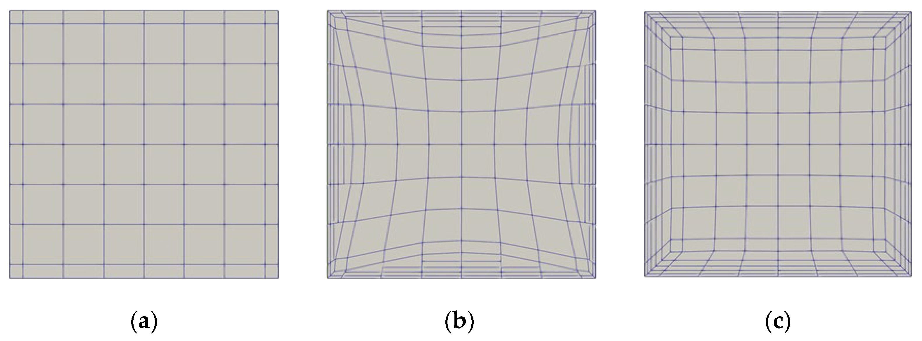
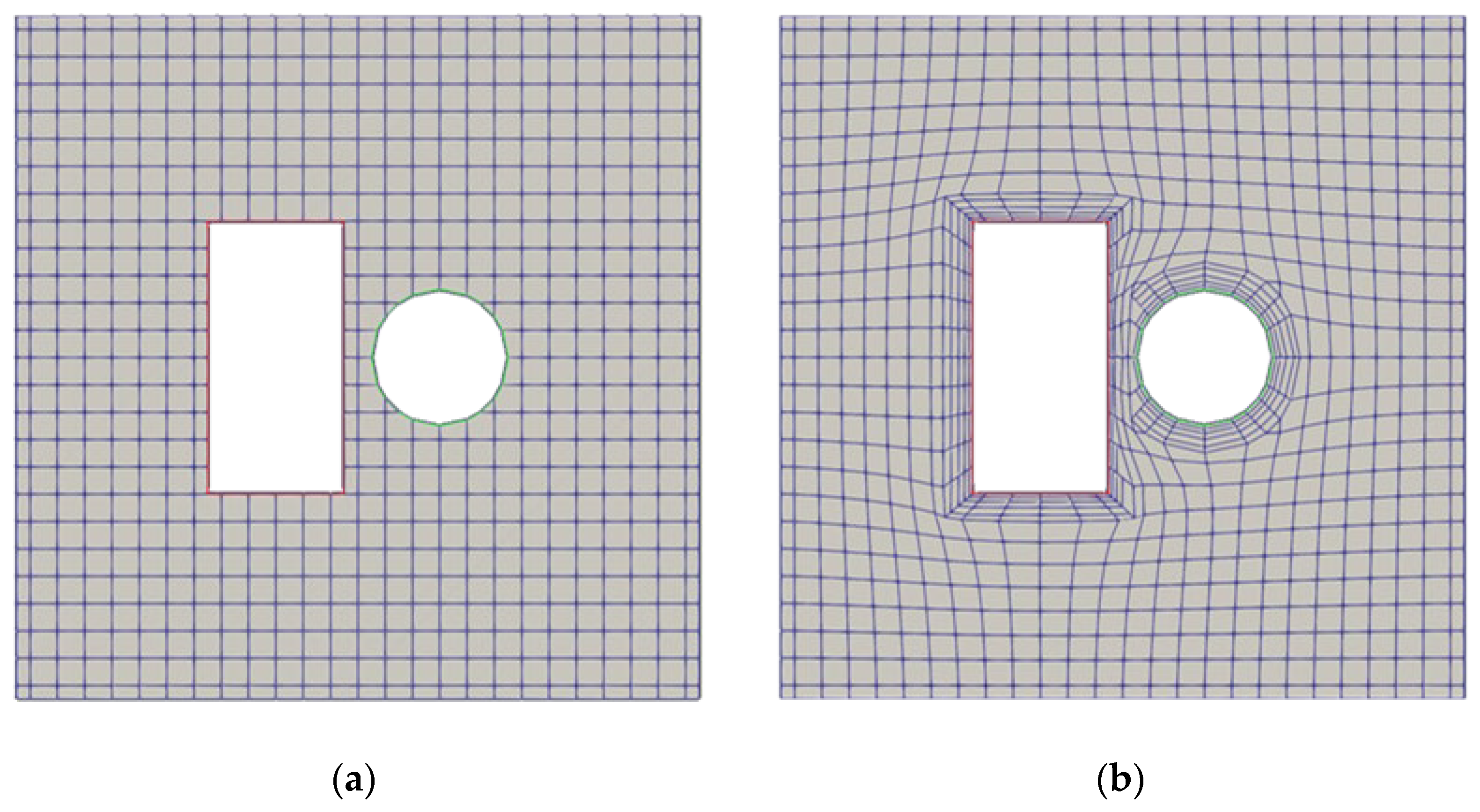
2.2. Front Advancing Technique

To avoid intersecting grid lines, i.e., a grid line of a mesh piercing through a grid line of another mesh, the front advancing technique is developed and applied.

2.2.1. Exclusion of Narrow Regions

To calculate the gradient fields of the displacement vectors of volume meshes, the Laplace equation in Equation (1) is solved using the initial displacement vector $\overrightarrow{D_0}$, which is the value of $\overrightarrow{D_b}$ multiplied by the thickness of the first boundary layer $t_{first}$ and is shown in Equation (6), as the boundary condition. The diffusion coefficient $\Gamma$ is determined by the reciprocal of the mesh’s volume. When the grid size is small, the gradient of the displacement reduces, and consequently, the deformation of the grid becomes relatively small. In contrast, when the grid size is large, the grid formation becomes relatively large. For the $\Gamma$ of the boundary layer grids, the adjacent volume mesh is used instead of the reciprocal of the volume. Through this, it is possible to avoid the problem of excessively deformed volume cell, which is due to the boundary grid and results in deterioration of the grid quality, or generation of excessively thin boundary layer grid. The values of $\Gamma$ are recalculated at every iteration due to volume change.

$$\overrightarrow{D_0}=\overrightarrow{D_b}·t_{first},$$

(6)

When the magnitude of the gradient of displacement is greater than 1, the corresponding grid face is judged to have a very narrow gap and is classified as the boundary grid face where the boundary layer is not generated. After checking the narrow gaps and considering classified grid surfaces without the boundary layer meshes, the smooth normal vector $\overrightarrow{SN}$ and displacement vector $\overrightarrow{D_b}$ are recalculated.

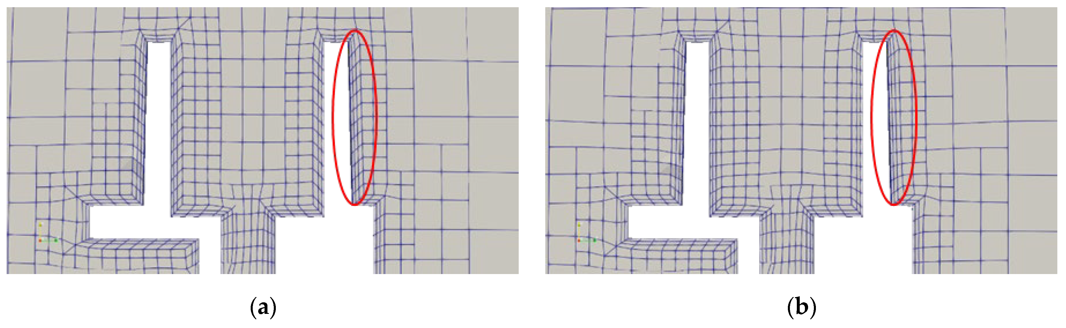
2.2.2. Gradual Front Advancing Method

The boundary layer grids are advanced by moving its grid points after copying the grid points of the boundary face to generate excessively thin boundary layer grids and calculating the displacement vector field of the volume mesh. To prevent the grid lines from intersecting, the amount of movement of the grid points is made to match that of displacement calculated at the moved position. Moreover, to avoid the grid from being excessively deformed and its quality being deteriorated in narrow gap regions, the value of Equation (6) was used for the initial displacement of the boundary face. Calculations are repeatedly carried out with the gradual increase in the displacement of the boundary faces in consideration of the thickness of the boundary layer grid while moving the grid points. Details on the process for preventing the grid lines from being intersected are as follows.

The displacement vector at the center of the grid is obtained by solving the Laplace equation. Furthermore, the displacement vector $\overrightarrow{D}$ of the grid point $p$, $\overrightarrow{D_{p_i}}$, is calculated by performing the weighted averaging method on the displacement vectors of the grids $c_j$ that contains the grid point. The weighting function—which is inversely proportional to the distance between the center point and displacement vector and proportional to the diffusion coefficient ${\Gamma }_j$—and its application for the $\overrightarrow{D_{p_i}}$ are shown in Equations (7) and (8), respectively. A temporary position $p^{temp}$ is calculated by adding the displacement vector $\overrightarrow{D}$ at the current grid point position to the initial grid position $p^0$ and under-relaxation is performed to calculate the new position of the grid point, as shown in Equations (9) and (10), which are iteratively solved. In the present study, 0.5 is used for the relaxation factor ω in Equation (10). Moving grid points in this manner does not cause problems of intersecting grid lines inside a continuous displacement vector field.

$$w_j=\frac{{\Gamma }_j}{\left|c_j-p_i\right|},$$

(7)

$$\overrightarrow{D_{p_i}}=\frac{{{\displaystyle \sum }}_j{w}_j\overrightarrow{D_{c_j}}}{{{\displaystyle \sum }}_j{w}_j},$$

(8)

$$p^{temp}=p^0+\overrightarrow{D_{p_i}},$$

(9)

$$p^n=\omega ·p^{n-1}+\left(1-\omega \right)·p^{temp},$$

(10)

If the thickness of the boundary layer grid is smaller or larger than the target value after moving the grid points, calculations are repeated by increasing or decreasing the displacement of the boundary faces until the thickness of the boundary layer grid approaches the target value. Once the thickness of the entire boundary layer grid is converged sufficiently, the grids are cut and split from the highest boundary layer grid line with a number of thin boundary layer grids. The grid is not cut if the grid thickness is less than 60% of the target thickness when the boundary layer grid is cut.

Figure 4a shows the initial volume mesh of a rectangular domain enclosed by four wall boundaries with four concave corners. The boundary layer grids generated near the wall boundaries using only normal vectors and smoothed normal vector together with displacement vectors are depicted in Figure 4a,b, respectively. It can be found that the boundary layer grids are generated as intended, although the grid line of the last boundary layer meshes is not perfectly flat, and some areas that are not perfectly perpendicular to the wall are observed.

The developed techniques are applied for the multiple bodies with a narrow gap between the bodies in a square domain. Figure 5a,b shows the initial volume mesh generated by the cut-cell method [11] and the final grid systems with boundary layer grids generated by present methods, respectively. From Figure 5b, it can be observed that the numbers of the boundary layer grids near the region where gap exists are reduced; the farther away from the gap, the greater the numbers. In addition, the grid sizes near the gap are similar to each other even when the volume decreases due to the deformation of the grid near the region. This is because the change of displacement is suppressed by adopting the method to use the diffusion coefficient Γ in Equation (1) as the reciprocal of the volume.

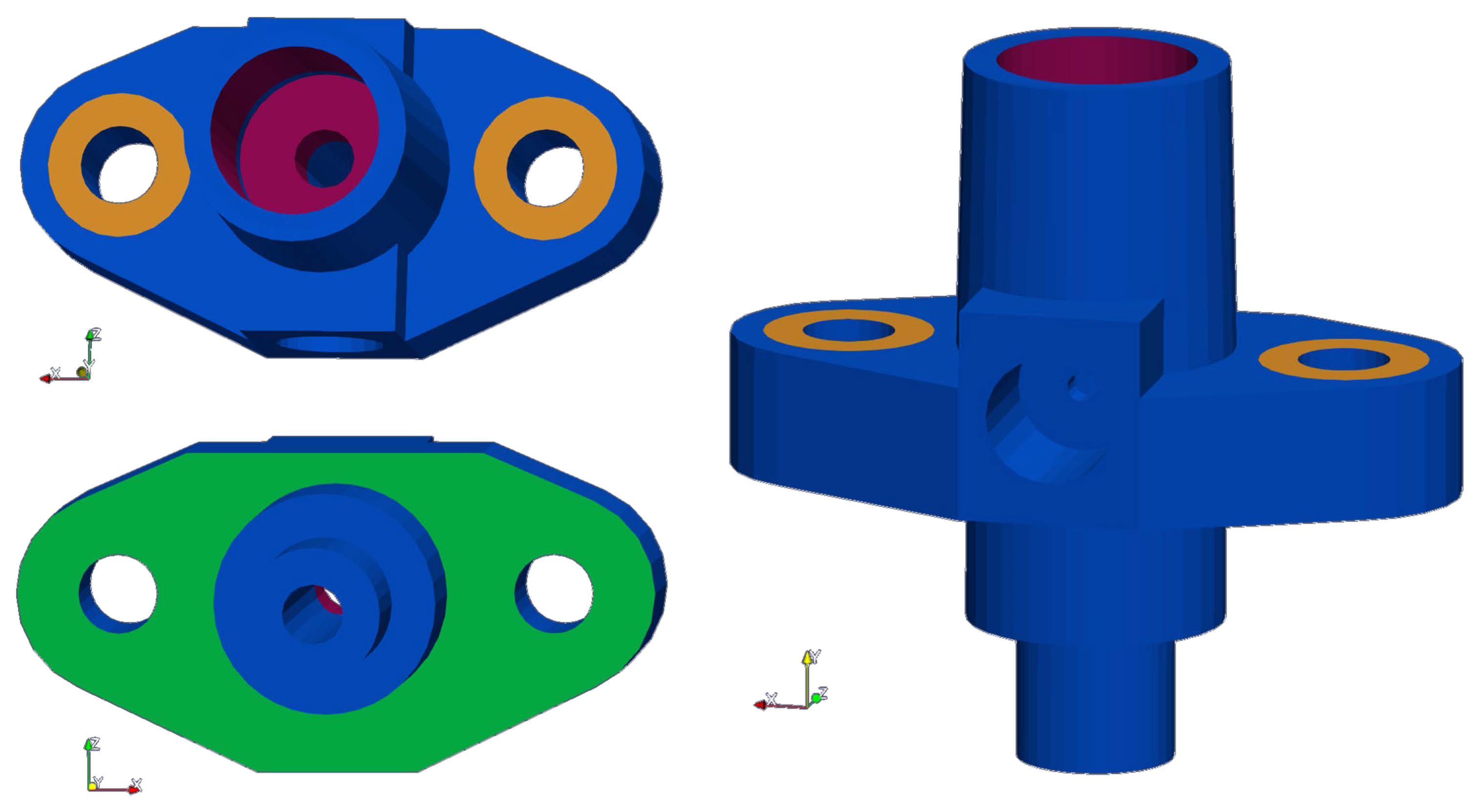
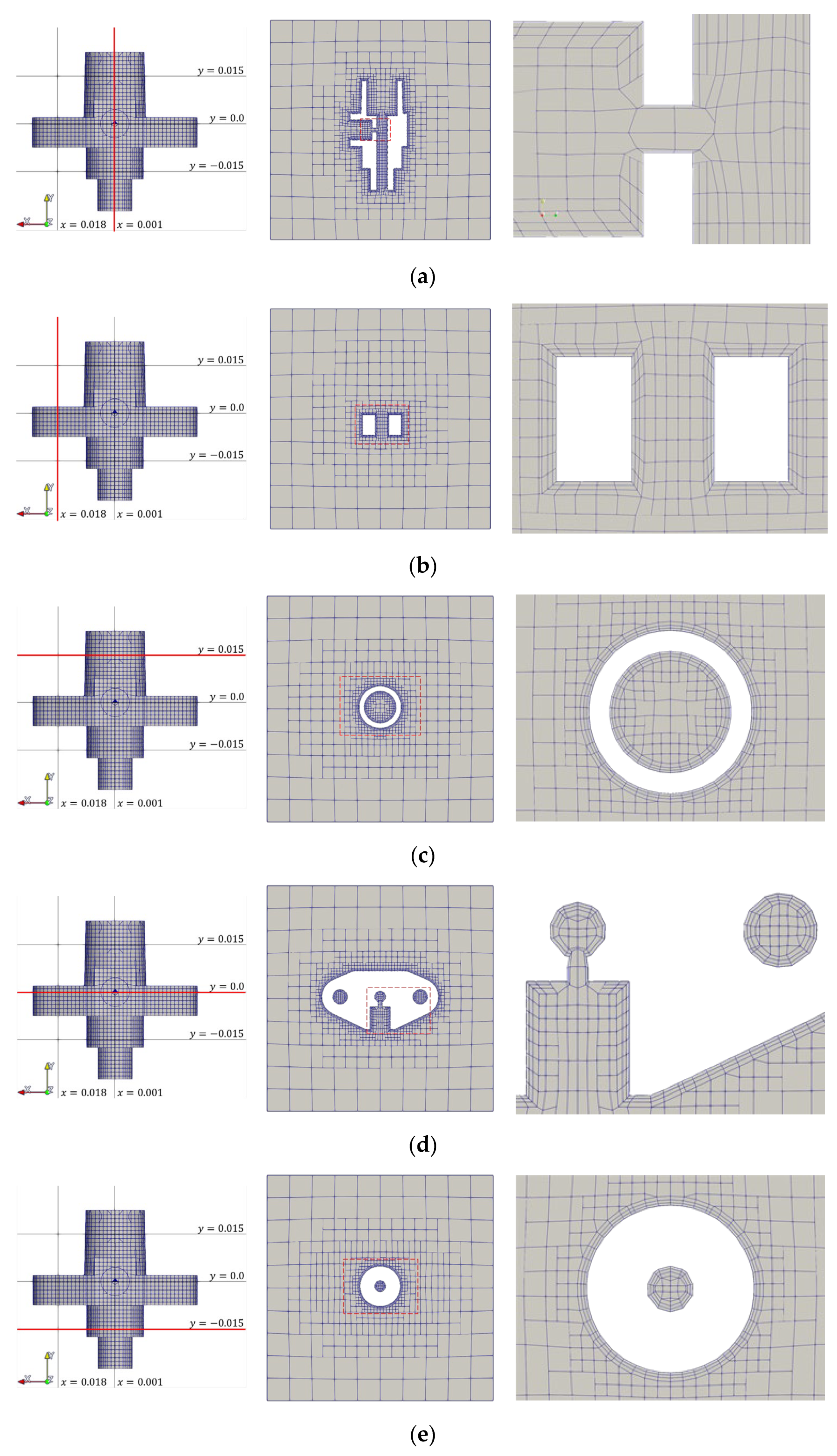
2.3. Applicatioon for Complex 3-D Geometry

The developed techniques are applied for a flange in a rectangular domain to check its applicability for a complex three-dimensional geometry. As shown in Figure 6, there are three holes in the y direction, of which the holes vary in size, and one hole that varies in size in the z direction.

To verify the validity of the developed method, relatively large-sized initial volume meshes were used to make it difficult to generate the boundary layer grids. For instance, the size of a hexahedral mesh on the surface of the flange is approximately 1.5 times that of the diameter of the small hole in the z-direction. The volume mesh and the boundary layer grids at several cross-sections are shown in Figure 7. In the figure, the boundary layer grids are well-generated at concave or convex corners, and grid lines do not intersect, even inside the relatively narrow holes. As shown in Figure 7a, only one boundary layer is created in the smallest hole where all the boundary layer grids cannot be inserted. In addition, from Figure 7d,e, the boundary layer grids are well-generated, even in small holes compared with that of the boundary layer.

As previously mentioned, the smoothed normal vector is calculated with the boundary conditions expressed in Equations (3) and (4) to select the normal vector at the corner edge and limit the smoothing region, respectively. The effects of limiting the smoothing region can be found in Figure 8, where the upper part of the grids on the $x=0.001$ plane is magnified and indicated. The orthogonality of the boundary layer grids without limiting, shown in Figure 8a, are much worse than those with limiting as shown in Figure 8b. The deformation of volume meshes in the first is slightly smaller than that in the latter since the restriction of smoothing region increases the difference between neighboring smoothed normal vectors. In short, it is found that the limiting technique improves the orthogonality of the boundary layer grids and increases the deformation of the volume meshes.

3. Numerical Simulations: Application to Propeller Open Water (POW) Test

The hydrodynamic performances of a marine vessel or floating type offshore structures can be categorized into seakeeping, maneuvering, and resistance and propulsion. Regarding the latter performance, tests of resistance, POW, and self-propulsion should be carried out to estimate the performance of a marine vessel. Although CFD has been traditionally and mainly applied to estimate the resistance and propulsion performance [11,16,17,18], it has been widening its range of application for other hydrodynamic cases [19,20] and more complicated problems related to resistance and propulsion, such as ship–ice interaction [21], energy-saving devices [22,23], hull form optimization [24], and so forth.

To check the applicability of the developed methods, numerical simulations of the POW test of a marine propeller were carried out. The initial volume mesh and boundary layer grid were generated by the fully polyhedral meshes on the basis of the trimmed hexahedral mesh [11] and proposed advancing layer method, respectively. The investigation on the generated grids is introduced, and then, the POW simulation results, which were performed by an open source CFD software OpenFOAM with the generated mesh, are explained and compared with other experimental and numerical results.

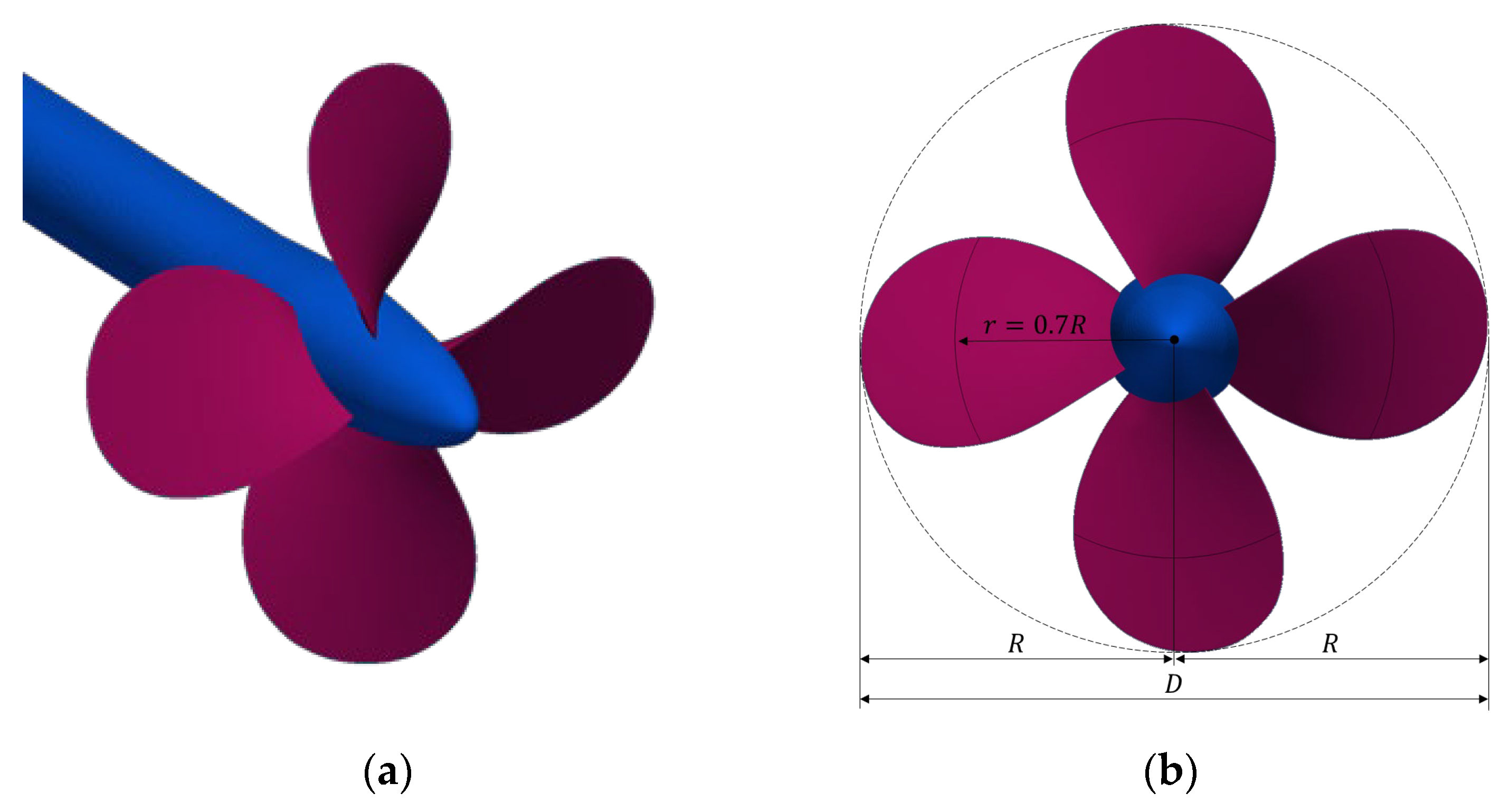
3.1. Subject Marine Propeller

In this study, the INSEAN E779A propeller, which was developed by INSEAN (Italian Ship Model Basin), was selected and used as the test-case propeller. The propeller is widely used in experimental studies under uniform and non-uniform flow conditions, and experimental results can be used as guidelines for validating the numerical test cases. The solid model of the propeller with a shaft is shown in Figure 9, where four very thin blades with skew and rake can be observed. The geometrical data of the propeller are listed in

Table 1. Geometrical characteristics of INSEAN E779A propeller.

Parameter (Unit)	Value
Diameter $\mathit{D}$ (m)	0.2272
Radius $\mathit{R}$ (m)	0.1136
Chord length at $r=0.7R$ ${\mathit{C}}_{\mathbf{0.7}\mathit{R}}$ (m)	0.086
Number of blades (-)	4
Pitch ratio (-)	1.1
Skew angle at the blade tip (°)	4.80 (positive)
Nominal rake (°)	4.59 (forward)
Expanded area ratio (-)	0.689
Hub diameter (m)	0.04553
Hub length (m)	0.06830

[25,26,27,28,29].

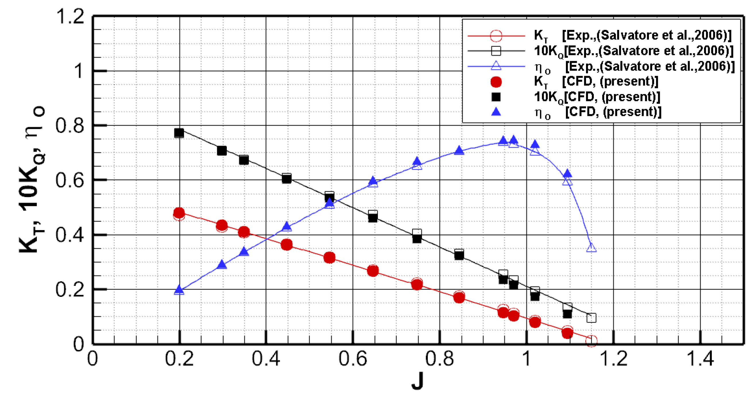
3.2. Non-Dimensional Coefficients

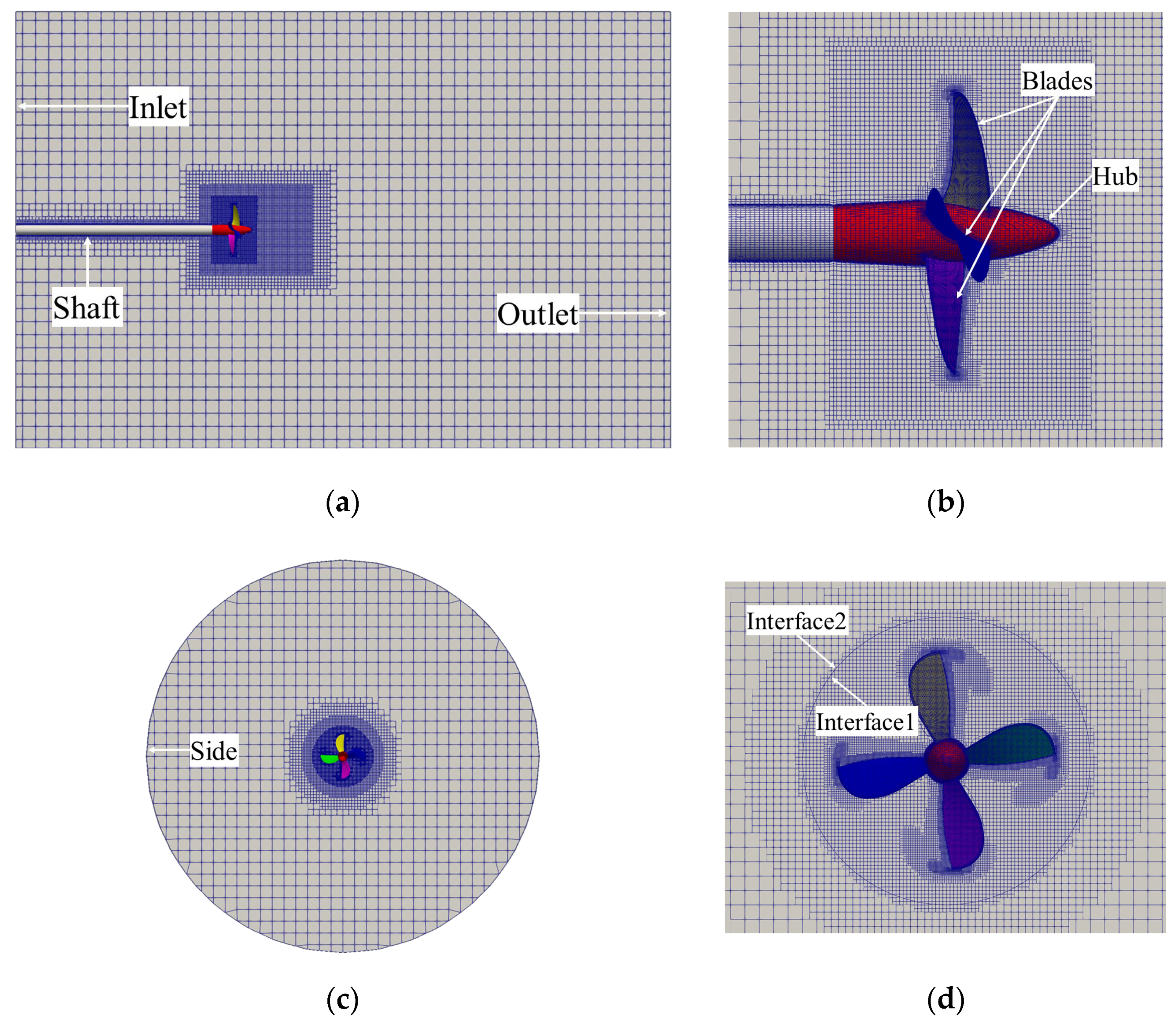
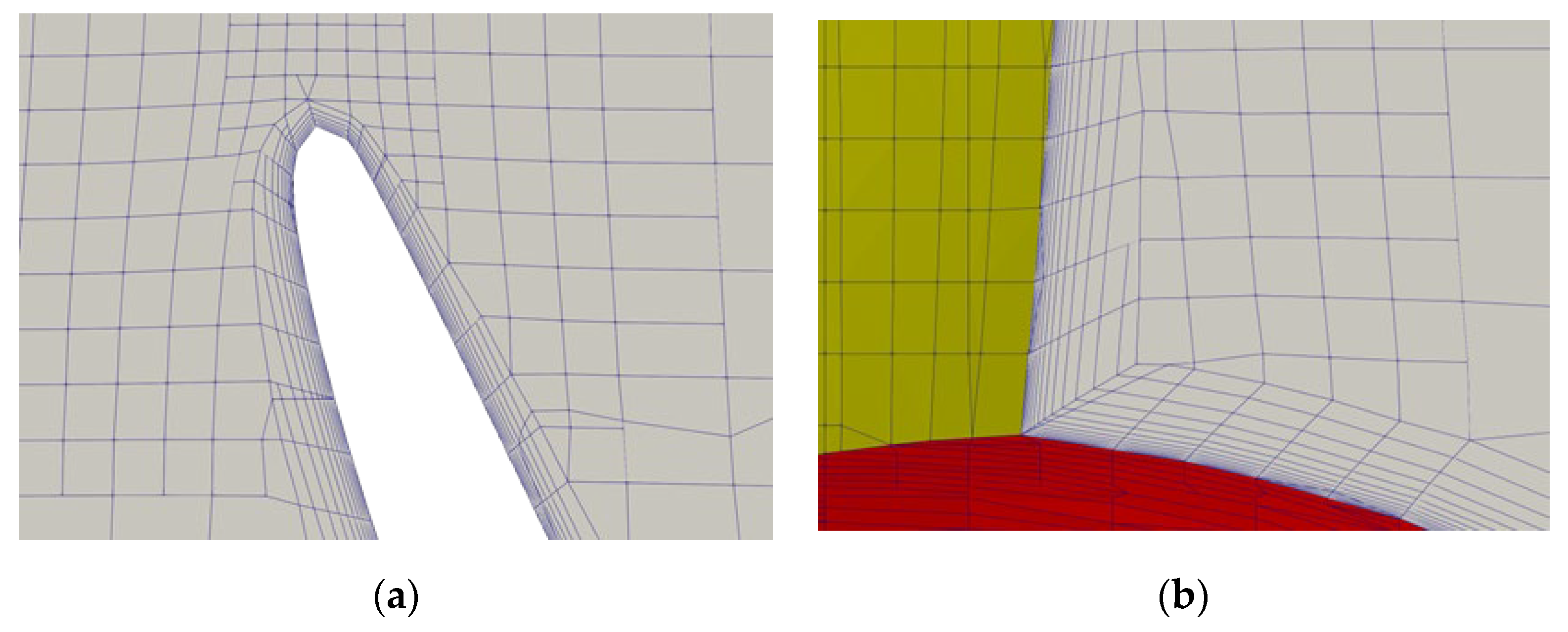
The non-dimensional coefficients relevant to the present simulation are introduced. Regarding the performance of a marine propeller, the important parameters are advance ratio $J$, thrust coefficient $K_T$, torque coefficient $K_Q$, and efficiency of the propeller ${\eta }_0$, which are defined as in Equations (11)–(14).

$$J=\frac{U_{\infty }}{nD}$$

(11)

$$K_T=\frac{T}{\rho n^2{D}^4}$$

(12)

$$K_Q=\frac{Q}{\rho n^2{D}^5}$$

(13)

$${\eta }_0=\frac{U_{\infty }T}{2\pi nQ}=\frac{J}{2\pi }\frac{K_T}{K_Q}$$

(14)

Here, $U_{\infty }$ is the inflow velocity, and $n$ and $D$ are the rotation rate and diameter of the propeller, respectively. $T$ and $Q$ are the thrust and torque of the propeller measured or estimated by numerical simulations, respectively. Furthermore, $\rho$ is the fluid density.

The Reynolds number for POW test $R{e}_{0.7R}$ is generally defined as shown in Equation (15) by the chord length $c$ and velocity considering the rotation speed of the blades, where the distance from the origin of the propeller $r$ is 0.7 times of the radius of the propeller, as shown in the Figure 9b.

$$R{e}_{0.7R}=\frac{C_{0.7R}·\sqrt{{\left(\pi ·D·0.7·R·n\right)}^2+U_{\infty }^2}}{\nu },$$

(15)

3.3. Grid Systems

Grid systems for the simulation of the POW tests of INSEAN E779A propeller were generated by the trimmed hexahedral mesh and the proposed advancing layer method for the initial volume meshes and boundary layer grids, respectively.

Figure 10 shows the generated grid systems where the figures in the left columns are the meshes of the entire domain, and the right columns are the magnified ones around the propeller. The upper and lower figures show those in the constant $y=0$ and $x=0$ planes, respectively. The region where the size of the volume meshes are larger than others, in which the same among them are fixed domains and others are multiple reference frame (MRF) domains, will be explained later. The total number of the grids was approximately $2.927\times {10}^6$, of which $2.889\times {10}^6$ were those of the rotating zone. The number of surface grids on a blade was 30,400. The length of the smallest volume mesh was approximately $2.3\times {10}^{-4} \mathrm{m}$. To preserve the shape of the propeller blades as precisely as possible and to detect the rapid change in the pressure and velocity near the leading and trailing edges of the blades, boundary layer grids were densely placed on the wall boundaries. The total number of the boundary layer grids was 14, with the extension ratio of 1.3. The height of the first boundary layer grid was $1.0\times {10}^{-5} \mathrm{m}$.

Figure 11 shows the boundary layer grids near the blade tip and root. In Figure 11a, it can be observed that the quality of the grids is quite good at the tip of the blade despite the existence of regions where the targeted number of the boundary layer grids, i.e., 14, are not generated because of small volume mesh and large $\Gamma$ in Equation (1). If all the boundary layer grids are forcefully placed around the tip, it gives rise to the problem of a boundary layer grid size larger than that of the volume mesh. As shown in Figure 11b, the boundary layer grids were not perfectly perpendicular to the boundary surfaces. However, the quality of the grids is acceptable where the blade root and hub meet with concave angle. Because the propeller pitch angle changes with respect to the distance from the origin of the propeller $r$ and the volume cell was different depending on the position, some regions were observed where the targeted number of the boundary layer grids were not generated. However, the authors believed that it did not significantly affect the simulation results. The mesh qualities were checked by checkMesh utility of OpenFOAM. The maximum aspect ratio was 374.8. The maximum and average non-orthogonality were 166.6 and 15.0, respectively. The maximum skewness was 191.2.

3.4. Solver, Schemes, and Conditions

For the POW tests, Reynolds-averaged Navier–Stokes equation (RANS) simulations with the transient turbulent model were performed. The solver used was simpleFoam, which is one of the standard solvers of Open Field Operation and Manipulation (OpenFOAM) 6 CFD toolbox. The simpleFoam is a steady-state solver for incompressible, turbulent flow using the SIMPLE (Semi-Implicit Method for Pressure Linked Equations) algorithm [30]. For the rotation of the propeller and shaft, the MRF method was chosen because this method is the simplest way of modeling for rotating multiple zones and suitable for present simulations. It is a steady-state approximation where there is no transient interaction between the rotating and static domains, as the mesh of the rotating part does not move.

The $\gamma -R{e}_{\theta }$ transition model [31,32,33] (kOmegaSSTLM in OpenFOAM) was adopted because the Reynolds numbers of the propeller $\mathit{R}{\mathit{e}}_{\mathbf{0.7}\mathit{R}}$ were in the laminar-to-turbulent transient regime. The turbulence intensity of the inflow was set to $1\%$ or less. To accelerate the computational time, the pressure and velocity fields obtained from the simulations by potentialFoam were used as for the initial values. Boundary conditions and numerical schemes are listed in

Table 2. Boundary conditions.

Boundaris	P	U	k	Omega	$\mathit{\gamma }$
Blade, hub, shaft	fixedFluxPressure	rotatingWallVelocity	kqRWallFunction	omegaWallFunction	zeroGradient
Inlet	zeroGradient	fixedValue
Outlet	fixedValue	zeroGradient
Interface1	cyclicAMI
Interface2	cyclicAMI
Side	symmetry

and

Table 3. Numerical schemes.

Convection Terms	Gauss Linear Upwind with Cell Limiter
Diffusion terms	Gauss linear
Matrix solver	Pressure: Geometric algebraic multi-grid (GAMG) with Gauss–Seidel smoother Other: smoothSolver with symGaussSeidel;

, respectively.

The speed of rotation $\mathit{n}$ was fixed and the inflow velocity ${\mathit{U}}_{\mathbf{\infty }}$ was determined to match the selected advance ratio $\mathit{J}$, which varied in the range of $0.119~1.094$. The corresponding Reynolds numbers were between $4.58\times {10}^5$ and $5.10\times {10}^5$, as listed in

Table 4. Simulation conditions.

Parameter (Unit)	Value
RPS of propeller $\mathit{n}$ (/s)	11.7881
Inflow velocity ${\mathit{U}}_{\mathbf{\infty }}$ (m/s)	0.533~2.931
Advance ratio $\mathit{J}$ (-)	0.199~1.094
Density of water $\mathit{\rho }$ (kg/m3)	1006.5
Dynamic viscosity of water $\mathit{\nu }$ (m2/s)	$1.1099\times {10}^{-6}$
Reynolds number at $r=0.7R {\mathit{R}\mathit{e}}_{\mathbf{0.7}\mathit{R}}$ (-)	$4.58\times {10}^5~5.10\times {10}^5$

.

3.5. Results

Figure 12 shows the comparisons between thrust and torque coefficients $K_T$ and $K_Q$ and propeller efficiency ${\eta }_0$ obtained from the present simulations and those of experiment [29]. From the figure, it can be observed that the results agree well with each other. Although a small discrepancy exists when the advance ratio $J$ is higher than 0.946, where the maximum value of ${\eta }_0$ is observed, it is a general tendency of most POW simulations. The error level of the present results is similar to that of the previous studies [34,35,36].

Figure 13 shows the distribution of $y^{+}$ and pressure on a blade surface when J = 0.946, where ${\eta }_0$ has the largest value. In the figure, face and back indicate the pressure side and suction side, respectively. The value of $y^{+}$ was approximately 3.2, which is slightly higher than 2.5, where the thickness of the first boundary layer was determined when generating grid systems. This slightly high value may be one of the reasons for the differences in thrust and torque.

From the results of checking the mesh qualities and simulations, it can be said that the developed advancing layer method is an appropriate method for generating the boundary layer grids of a trimmed hexahedral mesh. In addition, better results are expected by adjusting the boundary layer height with respect to the radius.

4. Conclusions

A robust and effective method based on the advancing layer method was developed to generate the boundary layer grids with non-intersecting grid lines near the wall boundaries where the concave corners and narrow gaps exist. The advancing layer method was modified and applied to the trimmed hexahedral volume meshes generated by the cut-cell method developed in the previous study. The Laplace equation of the normal and displacement vectors were used to smooth the normal vectors and obtain the displacement vector fields. The boundary layer grids were well-generated, even at the concave corner by smoothing the normal vectors of grid lines and faces. By utilizing the displacement vectors, the problem of intersecting grid lines in the narrow gap did not occur. The developed method was applied for a marine propeller, which has a complex geometry, and the propeller open water simulations were carried out with the generated grid system. Investigations on the grids and the simulation results compared with experimental results provide evidence of the applicability and effectiveness of the proposed method for practical problems. Further study will be carried out in the future to improve the quality of the present method, such as layer-by-layer generation of the boundary layer grids to make the grid lines more perpendicular to the wall boundaries.

References

1. Thompson, J.F.; Warsi, Z.U.; Mastin, C.W. Numerical Grid Generation: Foundations and Applications, 1st ed.; Elsevier North-Holland Inc.: Amsterdam, The Netherlands, 1985. [Google Scholar]
2. Mavriplis, D.J. Unstructured grid techniques. Annu. Rev. Fluid Mech. 1997, 29, 473–514. [Google Scholar] [CrossRef] [Green Version]
3. Eymard, R.; Gallouët, T.; Herbin, R. Finite volume methods. In Handbook of Numerical Analysis; Elsevier: Amsterdam, The Netherlands, 2000; Volume 7, pp. 713–1018. [Google Scholar]
4. Jeong, S.-M.; Lee, C.-Y. Weighted Moving Square-Based Solver for Unsteady Incompressible Laminar Flow Simulations. Appl. Sci. 2022, 12, 3519. [Google Scholar] [CrossRef]
5. Löhner, R.; Parikh, P. Generation of three-dimensional unstructured grids by the advancing-front method. Int. J. Numer. Methods Fluids 1988, 8, 1135–1149. [Google Scholar] [CrossRef]
6. Baker, T.J. Automatic mesh generation for complex three-dimensional regions using a constrained Delaunay triangulation. Eng. Comput. 1989, 5, 161–175. [Google Scholar] [CrossRef]
7. Thompson, J.F.; Soni, B.K.; Weatherill, N.P. Handbook of Grid Generation; CRC Press: Boca Raton, FL, USA, 1998. [Google Scholar]
8. Aftosmis, M.J.; Berger, M.J.; Melton, J.E. Robust and efficient cartesian mesh generation for component-based geometry. AIAA J. 1998, 36, 952–956. [Google Scholar] [CrossRef]
9. Nakahashi, K. Building-cube method for flow problems with broadband characteristic length. In Computational Fluid Dynamics; Springer: Berlin/Heidelberg, Germany, 2003; pp. 77–81. [Google Scholar]
10. Peskin, C.S. The immersed boundary method. Acta Numer. 2002, 11, 479–517. [Google Scholar] [CrossRef] [Green Version]
11. Jeong, K.-L.; Seo, D.-W. Automatic polyhedral mesh generation for ship resistance based on the locally refined cartesian cut-cell method. J. Mar. Sci. Technol. 2020, 28, 3. [Google Scholar]
12. Kim, H.-Y.; Kim, H.-G. A hexahedral-dominant FE meshing technique using trimmed hexahedral elements preserving sharp edges and corners. Eng. Comput. 2021, 38, 4307–4322. [Google Scholar] [CrossRef]
13. Wang, Z.; Quintanal, J.; Corral, R. Accelerating advancing layer viscous mesh generation for 3D complex configurations. Comput. Aided Des. 2019, 112, 35–46. [Google Scholar] [CrossRef]
14. Alauzet, F.; Loseille, A.; Marcum, D. On a robust boundary layer mesh generation process. In Proceedings of the 55th AIAA Aerospace Sciences Meeting, Grapevine, TX, USA, 9–13 January 2017. [Google Scholar]
15. Garimella, R.V.; Shephard, M.S. Boundary layer mesh generation for viscous flow simulations. Int. J. Numer. Methods Eng. 2000, 49, 193–218. [Google Scholar] [CrossRef]
16. Shin, M.-S.; Ki, M.-S.; Park, B.-J.; Lee, G.-J.; Lee, Y.-Y.; Kim, Y.; Lee, S.-B. Speed-Power Performance Analysis of an Existing 8,600 TEU Container Ship using SPA (Ship Performance Analysis) Program and Discussion on Wind-Resistance Coefficients. J. Ocean Eng. Technol. 2020, 34, 294–303. [Google Scholar] [CrossRef]
17. Grlj, C.G.; Degiuli, N.; Farkas, A.; Martić, I. Numerical Study of Scale Effects on Open Water Propeller Performance. J. Mar. Sci. Eng. 2022, 10, 1132. [Google Scholar] [CrossRef]
18. Jasak, H.; Vukčević, V.; Gatin, I.; Lalović, I. CFD validation and grid sensitivity studies of full scale ship self propulsion. Int. J. Nav. Archit. Ocean Eng. 2019, 11, 33–43. [Google Scholar] [CrossRef]
19. Jeong, S.-M.; Son, B.-H.; Lee, C.-Y. Estimation of the Motion Performance of a Light Buoy Adopting Ecofriendly and Lightweight Materials in Waves. J. Mar. Sci. Eng. 2020, 8, 139. [Google Scholar] [CrossRef] [Green Version]
20. Chen, C.; Zou, L.; Zou, Z.; Guo, H. Assessment of CFD-Based Ship Maneuvering Predictions Using Different Propeller Modeling Methods. J. Mar. Sci. Eng. 2022, 10, 1131. [Google Scholar] [CrossRef]
21. Song, S.; Park, S. Discrete Element Method Approach to Modeling Mechanical Properties of Three-Dimensional Ice Beams. J. Mar. Sci. Eng. 2022, 10, 1359. [Google Scholar] [CrossRef]
22. Ng’aru, J.-M.; Park, S. CFD Simulations of the Effect of Equalizing Duct Configurations on Cavitating Flow around a Propeller. J. Mar. Sci. Eng. 2022, 10, 1865. [Google Scholar] [CrossRef]
23. Kim, D.-H.; Park, J.-C.; Jeon, G.-M.; Shin, M.-S. CFD Simulation for Estimating Efficiency of PBCF Installed on a 176K Bulk Carrier under Both POW and Self-Propulsion Conditions. Processes 2021, 9, 1192. [Google Scholar] [CrossRef]
24. Jeong, K.-L.; Jeong, S.-M. A Mesh Deformation Method for CFD-Based Hull form Optimization. J. Mar. Sci. Eng. 2020, 8, 473. [Google Scholar] [CrossRef]
25. Pereira, F.; Di Felice, F.; Salvatore, F. Numerical investigation of the cavitation pattern on a marine propeller: Validation vs experiments. In Proceedings of the 23rd ITTC, Venice, Italy, 8–14 September 2002. [Google Scholar]
26. Pereira, F.; Salvatore, F.; Di Felice, F. Measurement and modeling of propeller cavitation in uniform inflow. J. Fluid Eng. 2004, 126, 671–679. [Google Scholar] [CrossRef]
27. Pereira, F.; Salvatore, F.; Di Felice, F.; Soave, M. Experimental investigation of a cavitating propeller in non-uniform inflow. In Proceedings of the Twenty-Fifth ONR Symposium on Naval Hydrodynamics, St. John’s, NL, Canada, 8–13 August 2004. [Google Scholar]
28. Salvatore, F.; Pereira, F.; Felli, M.; Calcagni, D.; Felice, F.D. Description of the INSEAN E779A Propeller Experimental Dataset. Technical Report 2006-085, INSEAN; 2006. Available online: https://www.researchgate.net/publication/259671974_Description_of_the_INSEAN_E779A_Propeller_Experimental_Dataset (accessed on 17 January 2023).
29. Salvatore, F.; Streckwall, H.; Terwisga, T. Propeller cavitation modeling by CFD results from the VIRTUE 2008. In Proceedings of the 1st International Symposium on Cavitation (SMP ’09), Trondheim, Norway, 22–24 June 2009; pp. 362–371. [Google Scholar]
30. Patankar, S.V. Numerical Heat Transfer and Fluid Flow; Taylor & Francis: Oxford, UK, 1980. [Google Scholar]
31. Menter, F.R.; Langtry, R.; Volker, S. Transition modelling for general purpose CFD codes. Flow Turbul. Combust. 2006, 77, 277–303. [Google Scholar] [CrossRef]
32. Langtry, R.B. A Correlation-Based Transition Model Using Local Variables for Unstructured Parallelized CFD Codes. Ph.D. Thesis, Universität Stuttgart, Stuttgart, Germany, 2006. [Google Scholar]
33. Langtry, R.B.; Menter, F.R. Correlation-based transition modeling for unstructured parallelized computational fluid dynamics codes. AIAA J. 2009, 47, 2894–2906. [Google Scholar]
34. Lingu, A. Scale effects on a tip rake propeller working in open water. J. Mar. Sci. Eng. 2019, 7, 404. [Google Scholar]
35. Moran-Guerrero, A.; Miguel Gonzalez-Gutierrez, L.M.; Oliva-Remola, A.; Diaz-Ojeda, H.R. On the influence of transition modeling and crossflow effects on open water propeller simulations. Ocean Eng. 2018, 156, 101–119. [Google Scholar] [CrossRef]
36. Andersson, J.; Eslamdoost, A.; Patrao, A.C.; Hyensjo, M.; Bensow, R.E. Energy balance analysis of a propeller in open water. Ocean Eng. 2018, 158, 162–170. [Google Scholar]
Figure 2. Schematic of (a) initial and (b) smoothed normal vectors of boundary grid lines and faces. Normal vectors inside the boxes are used for boundary conditions for the Laplace equation.
Jmse 11 00454 g002
Figure 3. (a) Initial normal vectors, (b) smoothed normal vectors, and (c) displacement vectors of boundary grid faces of the entire domain and near left bottom corner.
Jmse 11 00454 g003
Figure 4. (a) Initial volume mesh without boundary layer grids and final volume meshes with boundary grids generated using (b) normal vectors and (c) smoothed normal vectors together with displacement vectors.
Jmse 11 00454 g004
Figure 5. (a) Initial volume mesh without boundary layer grids and (b) final volume mesh with boundary layer grids for two bodies having a narrow gap between the bodies in a square domain.
Jmse 11 00454 g005
Figure 6. Geometry of a 3-D flange.
Jmse 11 00454 g006
Figure 7. Generated volume meshed in the constant planes of (a) x = 0.001, (b) x = 0.018, (c) y = 0.015, (d) y = 0.0, and (e) y = −0.015 for a 3-D flange in a rectangular domain where left, middle, and right columns indicate the plane position, grids on those plane, and the grids in the magnified region marked by red box in the middle one, respectively.
Jmse 11 00454 g007
Figure 8. Comparison of generated boundary layer grids in the constant plane of x = 0.001 (a) without and (b) with limiting smoothing region.
Jmse 11 00454 g008
Figure 9. Solid model of the INSEAN E779A propeller with shaft in (a) perspective and (b) front views.
Jmse 11 00454 g009
Figure 10. Grid systems of (a) whole and (b) magnified constant y = 0 plane and (c) whole and (d) magnified constant x = 0 plane for POW simulations.
Jmse 11 00454 g010
Figure 11. Boundary layer grids around (a) blade tip and (b) root and hub of the propeller.
Jmse 11 00454 g011
Figure 12. Comparisons of POW simulation results with experimental results.
Jmse 11 00454 g012
Figure 13. Contours maps of y + and pressure on blade surfaces of face and back when J = 0.946 : (a) face, (b) back, (c) face, and (d) back.
Jmse 11 00454 g013