
Phytoplankton of the High-Latitude Arctic: Intensive Growth Large Diatoms Porosira glacialis in the Nansen Basin

 , , ,
, , ,  ,
,
Abstract
:1. Introduction
- To obtain data on water masses and hydrophysical, hydrochemical, and optical properties of water;
- To investigate the phytoplankton composition in the MIZ area and open water at stations with different ratios of polar and Atlantic waters;
- To understand the mechanisms of increasing productivity in MIZ and to test the hypothesis about halocline’s determining role in forming a highly productive zone;
- Flora composition is a biomarker of the ice age, so knowing the phytoplankton allows us to test the following hypothesis: In the Nansen Basin, there was a significant shift in the ice cover formation, namely, the replacement of the multiyear ice with the first-year ice.
2. Methods
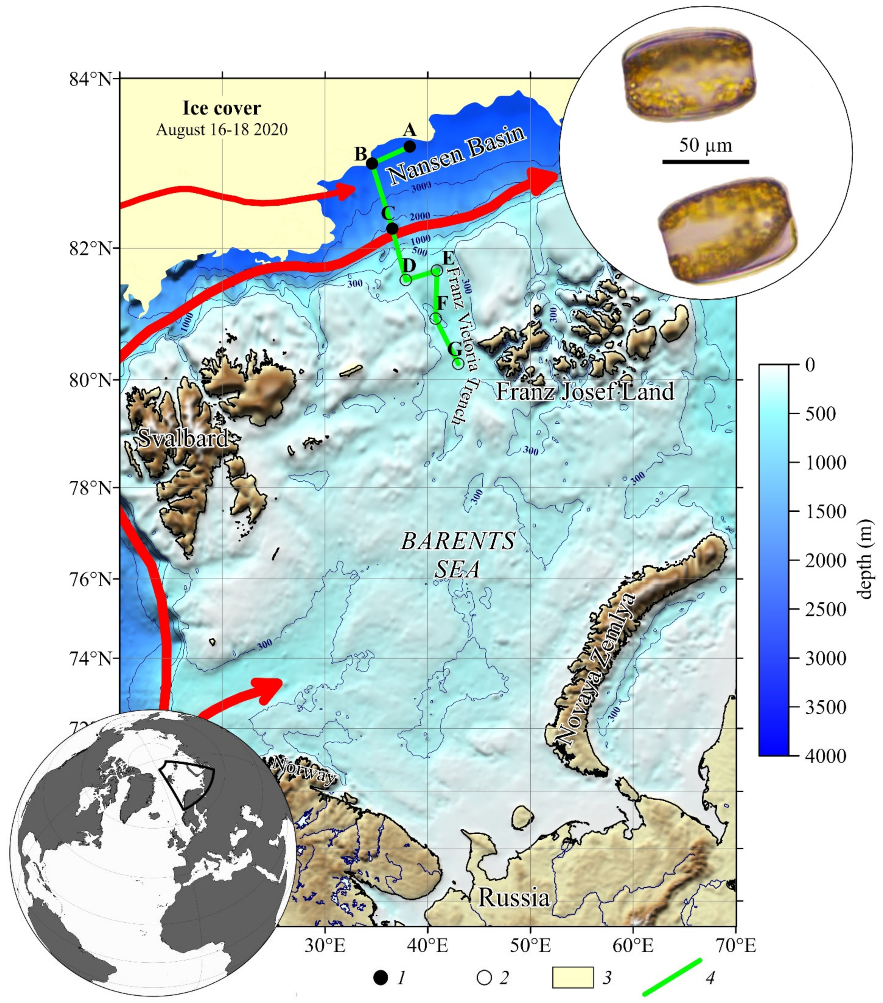
2.1. Field Studies
2.2. Species Identification
2.3. Nutrient Analyses and Chlorophyll a and Primary Production Determinations
2.4. Optical Measurements
3. Results
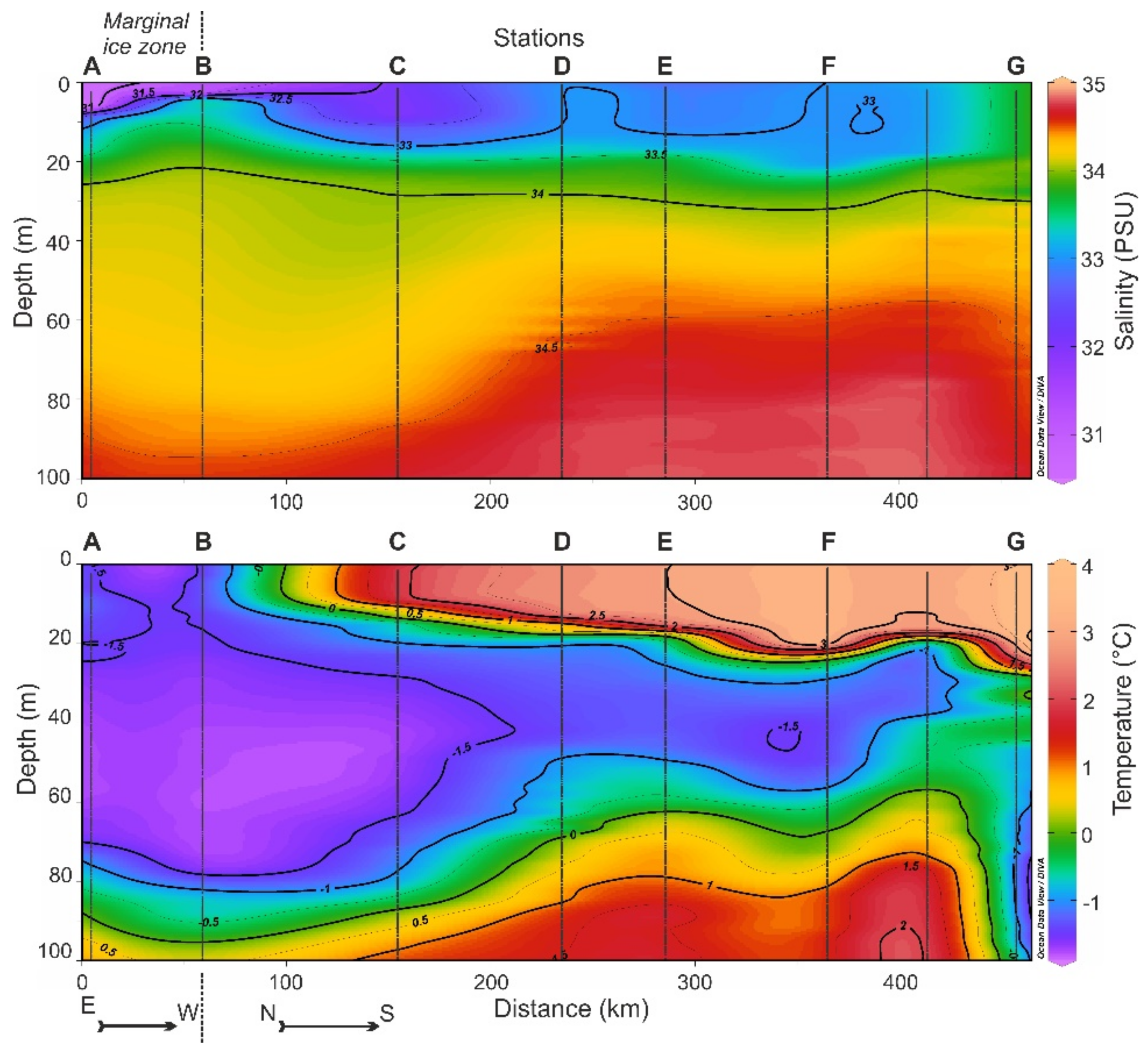
3.1. Hydrophysical Conditions
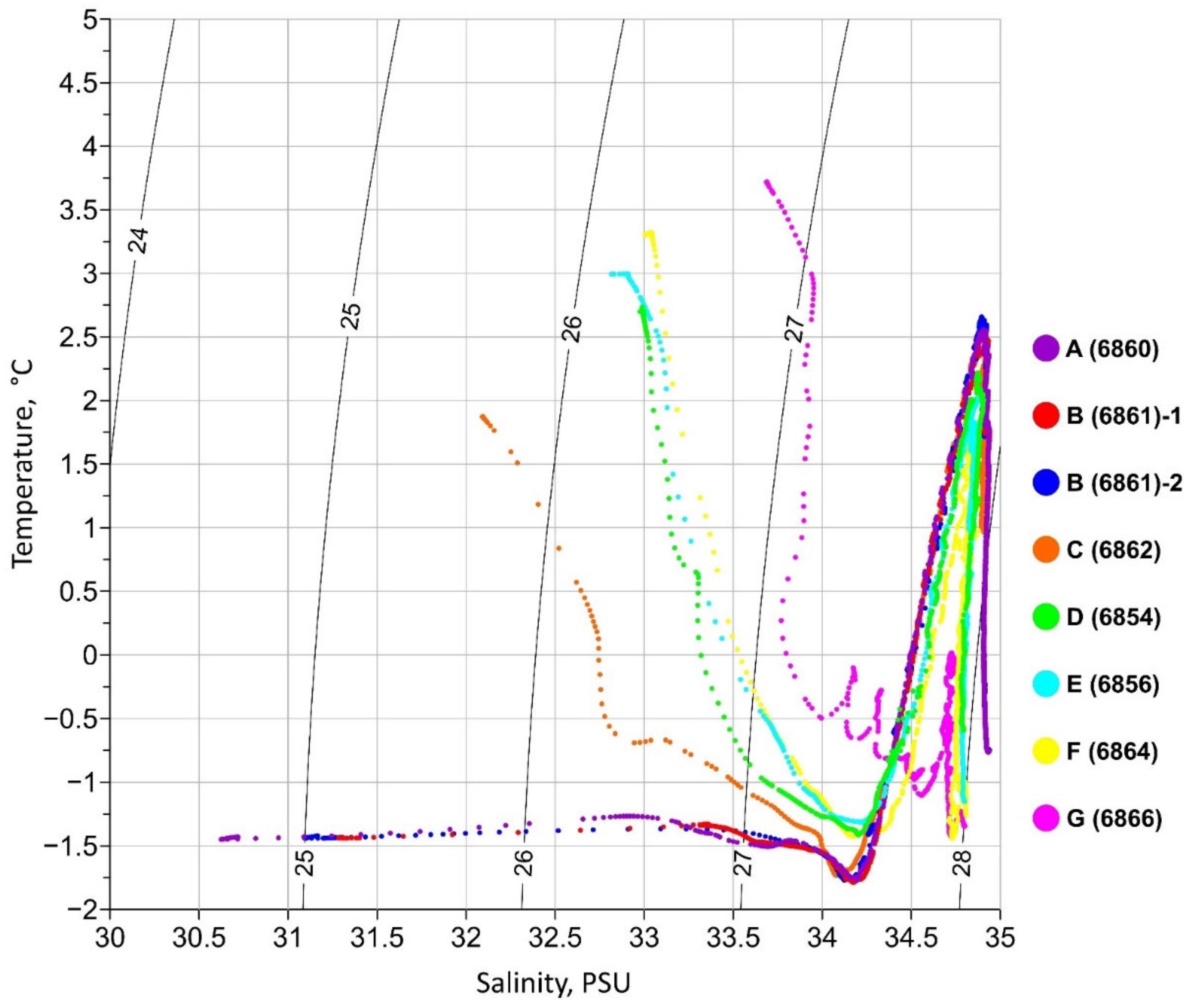
3.2. The Distribution of Water Masses
3.3. Hydrochemical Conditions
3.4. Light Conditions and Optical Characteristics of Water
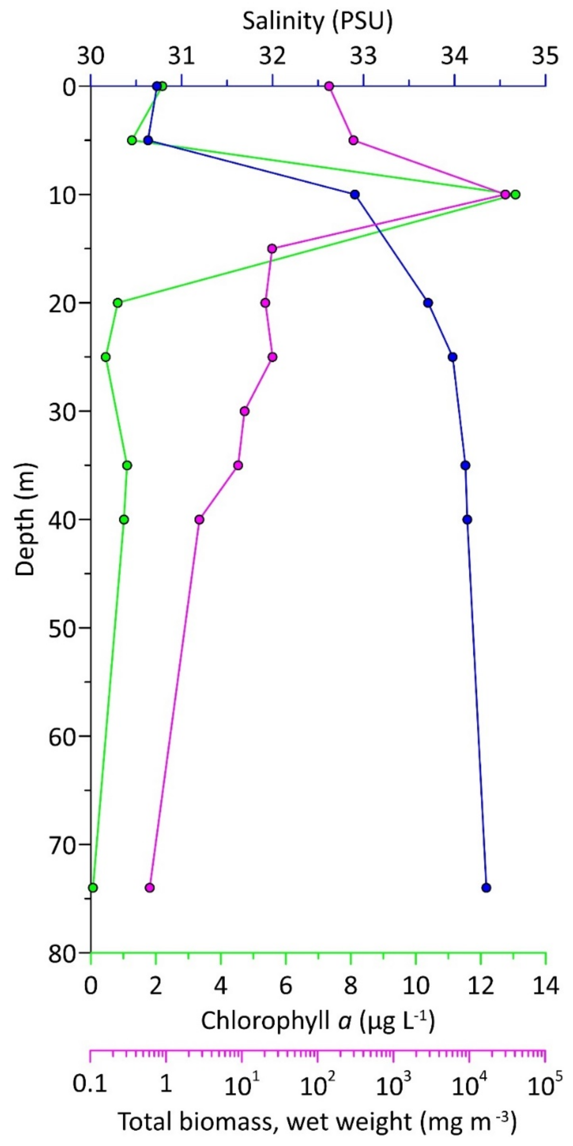
3.5. Structure and Biomass of Phytoplankton
- Species associated with the multiyear ice;
- Species associated with the first-year ice [26];
- Atlantic species of spring blooms in open-water areas (Chaetoceros gelidis, Eucampia groenlandica, Phaeocystis pouchettii, Pseudo-nitzschia delicatissima);
- Large Atlantic oceanic species of the summer complex from the genus Chaetoceros, Rhizosolenia and Sundstroemia.

| Stations | |||||||
|---|---|---|---|---|---|---|---|
| Species | A | B | C | D | E | F | G |
| I. The species associated with multiyear ice | |||||||
| 0 | ||||||
| 0–5 | ||||||
| 0, 20 | 3 | 0, 30 | ||||
| 0 | ||||||
| 0, 10, 30 | ||||||
| 0–5, 25 | ||||||
| 0–5 | 0–24 | 22 | ||||
| II. The species associated with second-year ice | |||||||
| 2 | ||||||
| III. The species associated with first-year ice | |||||||
| 0–25, 200, 800, 3000 | 0–15 | 602 | 7, 28–38 | 50–140 | 111, 571 | |
| 0–40, 74, 3000 | 0–15, 34–600 | 2–45, 100 | 20–38, 100, 400 | 40–100, | 100, 111, 571 | 66 |
| 0, 20 | 2–45 | 27–38 | 50, 140 | |||
| 0, 20 40 | 38–45, 100 | 200 | 140 | 111 | ||
| 0–35 | 6–45, 22–38 | |||||
| 20 | ||||||
| IV. The Atlantic open water species | |||||||
| 0–30 | 0–46, 72 | 2, 10, 30 | 38 | 10 | ||
| 0–25 | 16–45 | 27–38 | ||||
| 200 | 38–45 | 27–38 | 40 | |||
| 0–5 | 24 | |||||
| 0–25 | 38 | |||||
| 25–30, | 34, 72, 91 | |||||
| 5, 20–40 | 46, 72 | 0, 22, 30 | 7, 20, 27, 38 | 26–40 | ||
| 25–35 | 34–46, 72 | 30–38, 45 | ||||
| 10, 25, 30 | 46 | 30–38 | 7 | |||
| 46, 72 | 38–45 | |||||
| 30 | 46, 72 | 46 | 12 | |||
| 34, 46 | ||||||
| 20–30 | 0–46, 100 | 10 | 25–38 | 03.05.1940 | 4–30, 60 | 0, 4, 20 |
| 0, 20 | 0–30 | 0, 7, 12, 38 | 16–26 | |||
| 185 | ||||||
| 35 | 10, 602 | 0 | 0, 4, 20 | |||
| 200 | 28–45 | 27–38 | 40 | |||
| 2 | 0–100 | 0–40 | 4–100 | 0–20 | ||
4. Discussion
4.1. Environmental Conditions
4.2. Light Conditions and Optical Characteristics of Water
4.3. Changes in Hydrochemical Parameters at the Studied Stations
4.4. Structure, Abundance and Biomass of Phytoplankton
5. Conclusions
Supplementary Materials
Author Contributions
Funding
Institutional Review Board Statement
Informed Consent Statement
Data Availability Statement
Acknowledgments
Conflicts of Interest
References
- Carmack, E.; Melling, H. Warmth from the deep. Nat. Geosci. 2011, 4, 7–8. [Google Scholar] [CrossRef]
- Stroeve, J.C.; Serreze, M.C.; Holland, M.M.; Kay, J.E.; Malanik, J.; Barrett, A.P. The Arctic’s rapidly shrinking sea ice cover: A research synthesis. Clim. Chang. 2012, 110, 1005–1027. [Google Scholar] [CrossRef] [Green Version]
- Stroeve, J.; Notz, D. Changing state of Arctic sea ice across all seasons. Environ. Res. Lett. 2018, 13, 103001. [Google Scholar] [CrossRef]
- Onarheim, T.; Eldevik, I.H.; Smedsrud, L.H.; Stroeve, J.C. Seasonal and Regional Manifestation of Arctic Sea Ice Loss. J. Clim. 2018, 31, 4917–4932. [Google Scholar] [CrossRef]
- Pnyushkov, A.V.; Polyakov, I.V.; Alekseev, G.V.; Ashik, I.M.; Baumann, T.M.; Carmack, E.C.; Ivanov, V.V.; Rember, R. A Steady Regime of Volume and Heat Transports in the Eastern Arctic Ocean in the Early 21st Century. Front. Mar. Sci. 2021, 8, 705608. [Google Scholar] [CrossRef]
- Polyakov, I.V.; Pnyushkov, A.V.; Alkire, M.B.; Ashik, I.M.; Baumann, T.M.; Carmack, E.C.; Goszczko, I.; Guthrie, J.; Ivanov, V.V.; Kanzow, T.; et al. Greater role for Atlantic inflows on sea-ice loss in the Eurasian Basin of the Arctic Ocean. Science 2017, 536, 285–291. [Google Scholar] [CrossRef] [Green Version]
- Polyakov, I.V.; Rippeth, T.P.; Fer, I.; Baumann, T.M.; Carmack, E.C.; Ivanov, V.V.; Janout, M.; Padman, L.; Pnyushkov, A.V.; Rember, R. Intensification of Near-Surface Currents and Shear in the Eastern Arctic Ocean. Geophys. Res. Lett. 2020, 47, e2020GL089469. [Google Scholar] [CrossRef]
- Ivanov, V.V.; Repina, I.A. The effect of seasonal variability of Atlantic water on the Arctic Sea ice cover. Izv. Atmos. Ocean. Phys. 2018, 54, 65–72. [Google Scholar] [CrossRef]
- Årthun, M.; Eldevik, T.; Smedsrud, L.H.; Skagseth, O.; Ingvaldsen, R.B. Quantifying the Influence of Atlantic Heat on Barents Sea Ice Variability and Retreat. J. Clim. 2012, 25, 4736–4743. [Google Scholar] [CrossRef] [Green Version]
- Polyakov, I.V.; Rippeth, T.P.; Fer, I.; Alkire, M.B.; Baumann, T.M.; Carmack, E.C.; Ingvaldsen, R.; Ivanov, V.V.; Janout, M.; Lind, S.; et al. Weakening of cold halocline layer exposes sea ice to oceanic heat in the eastern arctic ocean. J. Clim. 2020, 33, 8107–8123. [Google Scholar] [CrossRef]
- Ivanov, V.V.; Tuzov, F.K. Formation of dense water dome over the Central Bank under conditions of reduced ice cover in the Barents Sea. Deep.-Sea Res. Part I Oceanogr. Res. Pap. 2021, 175, 103590. [Google Scholar] [CrossRef]
- Søreide, J.E.; Leu, E.; Berge, J.; Graeve, M.; Falk-Petersen, S. Timing in blooms, algal food quality and Calanus glacialis reproduction and growth in a changing Arctic. Glob. Change Biol. 2010, 16, 3154–3163. [Google Scholar] [CrossRef] [Green Version]
- Harada, N. Potential catastrophic reduction of sea ice in the western Arctic Ocean: Its impact on biogeochemical cycles and marine ecosystems. Glob. Planet. Change 2016, 136, 1–17. [Google Scholar] [CrossRef] [Green Version]
- Neukermans, G.; Oziel, L.; Babin, M. Increased intrusion of warming Atlantic water leads to a rapid expansion of temperate phytoplankton in the Arctic. Glob. Change Biol. 2018, 24, 2545–2553. [Google Scholar] [CrossRef]
- Oziel, L.; Sirven, J.; Gascard, J.C. The Barents Sea frontal zones and water masses variability (1980-2011). Ocean Sci. 2016, 12, 169–184. [Google Scholar] [CrossRef] [Green Version]
- Oziel, L.; Baudena, A.; Ardyna, M.; Massicotte, M.; Randelhoff, A.; Sallée, J.-B.; Ingvaldsen, R.B.; Devred, E.; Babin, M. Faster Atlantic currents drive poleward expansion of temperate phytoplankton in the Arctic Ocean. Nat. Commun. 2020, 11, 1705. [Google Scholar] [CrossRef] [Green Version]
- Randelhoff, A.; Sundfjord, A.; Reigstad, M. Seasonal variability and fluxes of nitrate in the surface waters over the Arctic shelf slope. Geophys. Res. Lett. 2015, 42, 3442–3449. [Google Scholar] [CrossRef] [Green Version]
- Randelhoff, A.; Reigstad, M.; Chierici, M.; Sundfjord, A.; Ivanov, V.; Cape, M.; Vernet, M.; Tremblay, J.-É.; Bratbak, G.; Kristiansen, S. Seasonality of the Physical and Biogeochemical Hydrography in the Inflow to the Arctic Ocean Through Fram Strait. Front. Mar. Sci. 2018, 5, 224. [Google Scholar] [CrossRef] [Green Version]
- Krisch, S.; Hopwood, M.J.; Roig, S.; Gerringa, L.J.A.; Middag, R.; Rutgers van der Loeff, M.M.; Petrova, M.V.; Lodeiro, P.; Colombo, M.; Cullen, J.T.; et al. Arctic–Atlantic exchange of the dissolved micronutrients iron, manganese, cobalt, nickel, copper and zinc with a focus on Fram Strait. Glob. Biogeochem. Cycles 2022, 36, e2021GB007191. [Google Scholar] [CrossRef]
- Ardyna, M.; Arrigo, K.R. Phytoplankton dynamics in a changing Arctic Ocean. Nat. Clim. Chang. 2020, 10, 892–903. [Google Scholar] [CrossRef]
- Ardyna, M.; Mundy, C.J.; Mayot, N.; Matthes, L.C.; Oziel, L.; Horvat, C.; Leu, E.; Assmy, P.; Hill, V.; Matrai, P.A.; et al. Under-Ice Phytoplankton Blooms: Shedding Light on the “Invisible” Part of Arctic Primary Production. Front. Mar. Sci. 2020, 7, 608032. [Google Scholar] [CrossRef]
- Arrigo, K.R.; van Dijken, G.; Pabi, S. Impact of shrinking Arctic ice cover on marine primary production. Geophys. Res. Lett. 2008, 35, L19603. [Google Scholar] [CrossRef]
- Arrigo, K.R.; van Dijken, G. Continued increases in Arctic Ocean primary production. Prog. Oceanogr. 2015, 136, 60–70. [Google Scholar] [CrossRef]
- Fernández-Méndez, M.; Katlein, C.; Rabe, B.; Nicolaus, M.; Peeken, I.; Bakker, K.; Flores, H.; Boetius, A. Photosynthetic production in the Central Arctic Ocean during the record sea-ice minimum in 2012. Biogeosciences 2015, 12, 3525–3549. [Google Scholar] [CrossRef] [Green Version]
- Kwok, R. Arctic Sea ice thickness, volume, and multiyear ice coverage: Losses and coupled variability (1958–2018). Environ. Res. Lett. 2018, 13, 105005. [Google Scholar] [CrossRef]
- Syvertsen, E.E. Ice algae in the Barents Sea: Types of assemblages, origin, fate and role in the ice-edge phytoplankton bloom. Polar Res. 1991, 10, 277–288. [Google Scholar] [CrossRef]
- Fernández-Méndez, M.; Olsen, L.M.; Kauko, H.M.; Meyer, A.; Rösel, A.; Merkouriadi, I.; Mundy, C.J.; Ehn, J.K.; Johansson, A.M.; Wagner, P.M.; et al. Algal hot spots in a changing Arctic Ocean: Seaice ridges and the snow-ice interface. Front. Mar. Sci. 2018, 5, 75. [Google Scholar] [CrossRef] [Green Version]
- Hop, H.; Vihtakari, M.; Bluhm, B.A.; Assmy, P.; Poulin, M.; Gradinger, R.; Peeken, I.; von Quillfeldt, C.; Olsen, L.M.; Zhitina, L.; et al. Changes in Sea-Ice Protist Diversity with Declining Sea Ice in the Arctic Ocean From the 1980s to 2010s. Front. Mar. Sci. 2020, 7, 243. [Google Scholar] [CrossRef]
- Perrette, M.; Yool, A.; Quartly, G.D.; Popova, E.E. Near-ubiquity of ice-edge blooms in the Arctic. Biogeosciences 2011, 8, 515–524. [Google Scholar] [CrossRef] [Green Version]
- Slagstad, D.; Wassmann, P.F.J.; Ellingsen, I. Physical constrains and productivity in the future arctic ocean. Front. Mar. Sci. 2015, 2, 85. [Google Scholar] [CrossRef] [Green Version]
- Lewis, K.M.; van Dijken, G.L.; Arrigo, K.R. Changes in phytoplankton concentration now drive increased Arctic Ocean primary production. Science 2020, 369, 198–202. [Google Scholar] [CrossRef]
- Lind, S.; Ingvaldsen, R.B.; Furevik, T. Arctic warming hotspot in the northern Barents Sea linked to declining sea-ice import. Nat. Clim. Chang. 2018, 8, 634–639. [Google Scholar] [CrossRef]
- Schlichtholz, P. Subsurface Ocean flywheel of coupled climate variability in the Barents Sea hotspot of global warming. Sci. Rep. 2019, 9, 13692. [Google Scholar] [CrossRef] [Green Version]
- Oziel, L.; Neukermans, G.; Ardyna, M.; Lancelot, C.; Tison, J.-L.; Wassmann, P.; Sirven, J.; Ruiz-Pino, D.; Gascard, J.-C. Role for Atlantic inflows and sea ice loss on shifting phytoplankton blooms in the Barents Sea. J. Geophys. Res. Oceans 2017, 122, 5121–5139. [Google Scholar] [CrossRef] [Green Version]
- Winter, A.; Henderiks, J.; Beaufort, L.; Rickaby, R.E.M.; Brown, C.W. Poleward expansion of the coccolithophore Emiliania huxleyi. J. Plankton Res. 2014, 36, 316–325. [Google Scholar] [CrossRef]
- Silkin, V.; Pautova, L.; Giordano, M.; Kravchishina, M.; Artemiev, V. Interannual variability of Emiliania huxleyi blooms in the Barents Sea: In situ data 2014–2018. Mar. Pollut. Bull. 2020, 158, 111392. [Google Scholar] [CrossRef]
- Hegseth, E. Sub-ice algal assemblages of the Barents Sea: Species composition, chemical composition, and growth rates. Polar Biol. 1992, 12, 485–496. [Google Scholar] [CrossRef]
- Hegseth, E.N.; Sundfjord, A. Intrusion and blooming of Atlantic phytoplankton species in the high Arctic. J. Mar. Syst. 2008, 74, 108–119. [Google Scholar] [CrossRef]
- Owrid, G.; Socal, G.; Civitarese, G.; Luchetta, A.; Wiktor, J.; Nöthig, E.-M.; Andreassen, I.; Schauer, U.; Strass, V. Spatial variability of phytoplankton, nutrients and new production estimates in the waters around Svalbard. Polar Res. 2000, 19, 155–171. [Google Scholar] [CrossRef]
- Pautova, L.A. Phytoplankton of the Barets Sea. In System of the Barets Sea; GEOS: Moscow, Russia, 2021; pp. 317–330. [Google Scholar] [CrossRef]
- Hop, H.; Assmy, P.; Wold, A.; Sundfjord, A.; Daase, M.; Duarte, P.; Kwasniewski, S.; Gluchowska, M.; Wiktor, J.M.; Tatarek, A.; et al. Pelagic Ecosystem Characteristics Across the Atlantic Water Boundary Current from Rijpfjorden, Svalbard, to the Arctic Ocean During Summer (2010–2014). Front. Mar. Sci. 2019, 6, 181. [Google Scholar] [CrossRef]
- Onarheim, I.H.; Smedsrud, L.H.; Ingvaldsen, R.B.; Nilsen, F. Loss of sea ice during winter north of Svalbard. Tellus A 2014, 66, 23933. [Google Scholar] [CrossRef] [Green Version]
- Aksenov, P.V.; Ivanov, V.V. “Atlantification” as a Possible Cause for Reducing of the Sea-Ice Cover in the Nansen Basin in winter. Arct. Antarct. Res. 2018, 64, 42–54. (In Russian) [Google Scholar] [CrossRef] [Green Version]
- Renner, A.H.H.; Sundfjord, A.; Janout, M.A.; Ingvaldsen, R.B.; Beszczynska-Möller, A.; Pickart, R.S.; Pérez-Hernández, M.D. Variability and redistribution of heat in the Atlantic water boundary current north of Svalbard. J. Geophys. Res.-Oceans 2018, 123, 6373–6391. [Google Scholar] [CrossRef] [Green Version]
- Zenkevich, L.A. Biology of the Seas of the USSR; Georg Allen & Unwin: London, UK, 1963; p. 955. [Google Scholar]
- Tomas, C.R. (Ed.) Identifying Marine Phytoplankton; Academic Press: San Diego, CA, USA, 1997; 858p, ISBN 0-12-693018-X. [Google Scholar]
- Throndsen, J.; Hasle, G.R.; Tangen, K. Norsk Kystplanktonflora; Almater: Oslo, Norway, 2003; p. 341. [Google Scholar]
- Hillebrand, H.; Durselen, C.; Kirschtel, D.; Pollingher, U.; Zohary, T. Biovolume calculation for pelagic and benthic microalgae. J. Phycol. 1999, 35, 403–424. [Google Scholar] [CrossRef]
- Menden-Deuer, S.; Lessard, E.J. Carbon to volume relationship for dinoflagellates, diatom, and other protist plahkton. Limnol. Oceanogr. 2000, 45, 569–579. [Google Scholar] [CrossRef] [Green Version]
- Bordovskiy, O.K.; Chernyakova, A.M. (Eds.) Modern Methods of the Ocean Hydrochemical Investigations; P.P. Shirshov Institute of Oceanology: Moscow, Russia, 1992; 200p. (In Russian) [Google Scholar]
- Grashoff, K.; Kremling, K.; Ehrhard, M. Methods of Seawater Analysis; Wiley-VCH: Weinheim, Germany, 1999; 420p. [Google Scholar]
- Holm-Hansen, O.; Riemann, B. Chlorophyll a determination: Improvements in methodology. Oikos 1978, 30, 438–447. [Google Scholar] [CrossRef]
- Steemann-Nielsen, E. The use of radio-active carbon (14C) for measuring organic production in the sea. ICES J. Mar. Sci. 1952, 18, 117–140. [Google Scholar] [CrossRef]
- Kirk, J.T.O. Light and Photosynthesis in Aquatic Ecosystems, 3rd ed.; Cambridge University Press: New York, NY, USA, 2011; 649p. [Google Scholar]
- Perez-Hernandez, M.D.; Pickart, R.S.; Pavlov, V.; Våge, K.; Ingvaldsen, R.; Sundfjord, A.; Renner, A.H.H.; Torres, D.J.; Erofeeva, S.Y. The Atlantic Water boundary current north of Svalbard in late summer. J. Geophys. Res. Oceans 2017, 122, 2269–2290. [Google Scholar] [CrossRef]
- Kravchishina, M.D.; Klyuvitkin, A.A.; Volodin, V.D.; Glukhovets, D.I.; Dubinina, E.O.; Kruglinskii, I.A.; Kudryavtseva, E.A.; Matul, A.G.; Novichkova, E.A.; Politova, N.V.; et al. Systems Research of Sedimentation in the European Arctic in the 84th Cruise of the Research Vessel Akademik Mstislav Keldysh. Oceanology 2022, 62, 572–574. [Google Scholar] [CrossRef]
- Ivanov, V.V.; Alekseev, V.A.; Alekseeva, T.A.; Koldunov, N.V.; Repina, I.A.; Smirnov, A.V. Does the Arctic ice cover become seasonal? Earth Explor. Space 2013, 4, 50–65. (In Russian) [Google Scholar] [CrossRef]
- Ivanov, V.; Alexeev, V.; Koldunov, N.V.; Repina, I.A.; Sandoe, A.B.; Smedsrud, L.H.; Smirnov, A. Arctic Ocean heat impact on regional ice decay: Suggested positive feedback. J. Phys. Oceanogr. 2016, 46, 1437–1456. [Google Scholar] [CrossRef]
- Beszczynska-Möller, A.; Fahrbach, E.; Schauer, U.; Hansen, E. Variability in Atlantic water temperature and transport at the entrance to the Arctic Ocean, 1997–2010. ICES J. Mar. Sci. 2012, 69, 852–863. [Google Scholar] [CrossRef] [Green Version]
- Våge, K.; Pickart, R.S.; Pavlov, V.; Lin, P.; Torres, D.J.; Ingvalsen, I.; Sundjord, A.; Proshutinsky, A. The Atlantic Water boundary current in the Nansen Basin east of Fram Strait. J. Geophys. Res. Oceans 2016, 121, 6946–6960. [Google Scholar] [CrossRef] [Green Version]
- Rudels, B.; Korhonen, M.; Schauer, U.; Pisarev, S.; Rabe, B.; Wisotzki, A. Circulation and transformation of Atlantic water in the Eurasian Basin and the contribution of the Fram Strait inflow branch to the Arctic Ocean heat budget. Prog. Oceanogr. 2015, 132, 128–152. [Google Scholar] [CrossRef] [Green Version]
- Geider, R.J.; MacIntyre, H.L.; Kana, T.M. A dynamic regulatory model of phytoplankton acclimation to light, nutrients and temperature. Limnol. Oceanogr. 1998, 43, 679–694. [Google Scholar] [CrossRef]
- Falkowski, P.G.; LaRoche, J. Acclimation to spectral irradiance in algae. J. Phycol. 1991, 27, 8–14. [Google Scholar] [CrossRef]
- Falkowski, P.G.; Owens, T.G. Light–shade adaptation: Two strategies in marine phytoplankton. Plant Physiol. 1980, 66, 592–595. [Google Scholar] [CrossRef] [Green Version]
- MacIntyre, H.L.; Kana, T.M.; Anning, J.; Geider, R. Photoacclimation of photosynthesis irradiance response curves and photosynthetic pigments in microalgae and cyanobacteria. J. Phycol. 2002, 38, 17–38. [Google Scholar] [CrossRef] [Green Version]
- Jassby, A.D.; Platt, T. Mathematical formulation of the relationship between photosynthesis and light for phytoplankton. Limnol. Oceanogr. 1976, 21, 540–547. [Google Scholar] [CrossRef] [Green Version]
- Geider, R.J.; Moore, C.M.; Ross, O.N. The role of cost–benefit analysis in models of phytoplankton growth and acclimation. Plant Ecol. Divers. 2009, 2, 165–178. [Google Scholar] [CrossRef]
- Silkin, V.; Fedorov, A.; Flynn, K.J.; Paramonov, L.; Pautova, L. Protoplasmic streaming of chloroplasts enables rapid photoacclimation in large diatoms. J. Plankton Res. 2021, 43, 831–845. [Google Scholar] [CrossRef]
- Edwards, K.F.; Thomas, M.K.; Klausmeier, C.A.; Litchman, E. Phytoplankton growth and the interactionof light and temperature: A synthesis at the species and community level. Limnol. Oceanogr. 2016, 61, 1232–1244. [Google Scholar] [CrossRef] [Green Version]
- Allen, J.G.; Dugenne, M.; Letelier, R.M.; White, A.E. Optical determinations of photophysiology along an ecological gradient in the North Pacific Ocean. Limnol. Oceanogr. 2022, 7, 713–725. [Google Scholar] [CrossRef]
- Bouman, H.A.; Platt, T.; Doblin, M.; Figueiras, F.G.; Gudmundsson, K.; Gudfinnsson, H.G.; Huang, B.; Hickman, A.; Hiscock, M.; Jackson, T.; et al. Photosynthesis–irradiance parameters of marine phytoplankton: Synthesis of a global data set. Earth Syst. Sci. 2018, 10, 251–266. [Google Scholar] [CrossRef] [Green Version]
- Sakshaug, E.; Slagstad, D. Light and productivity of phytoplankton in polar marine ecosystems: A physiological view. Polar Res. 1991, 10, 69–85. [Google Scholar] [CrossRef]
- Torres-Valdes, S.; Tsubouchi, T.; Bacon, S.; Naveira-Garabato, A.C.; Sanders, R.; McLaughlin, F.A.; Petrie, B.; Kattner, G.; Azetsu-Scott, K.; Whitledge, T.E. Export of nutrients from the Arctic Ocean. J. Geophys. Res.-Oceans 2013, 118, 1625–1644. [Google Scholar] [CrossRef] [Green Version]
- Tremblay, J.E.; Anderson, L.G.; Matrai, P.; Coupel, P.; Belanger, S.; Michel, C.; Reigstad, M. Global and regional drivers of nutrient supply, primary production and CO2 drawdown in the changing Arctic Ocean. Prog. Oceanogr. 2015, 139, 171–196. [Google Scholar] [CrossRef]
- Henley, S.F.; Porter, M.; Hobbs, L.; Braun, J.; Guillaume-Castel, R.; Venables, E.J.; Dumont, E.; Cottier, F. Nitrate supply and uptake in the Atlantic Arctic sea ice zone: Seasonal cycle, mechanisms and drivers. Phil. Trans. R. Soc. A 2020, 378, 20190361. [Google Scholar] [CrossRef]
- Lewis, K.M.; Arntsen, A.E.; Coupel, P.; Joy-Warren, H.; Lowry, K.E.; Matsuoka, A.; Mills, M.M.; van Dijken, G.L.; Selz, V.; Arrigo, K.R. Photoacclimation of Arctic Ocean phytoplankton to shifting light and nutrient limitation. Limnol. Oceanogr. 2019, 64, 284–301. [Google Scholar] [CrossRef]
- Mills, M.M.; Brown, Z.W.; Laney, S.R.; Ortega-Retuerta, E.; Lowry, K.E.; van Dijken, G.L.; Arrigo, K.R. Nitrogen limitation of the summer phytoplankton and heterotrophic prokaryote communities in the Chukchi Sea. Front. Mar. Sci. 2018, 5, 362. [Google Scholar] [CrossRef] [Green Version]
- Falk-Petersen, S.; Hop, H.; Budgell, W.P.; Hegseth, E.N.; Korsnes, R.; Løyning, T.B.; Ørbæk, J.B.; Kawamura, T.; Shirasawa, K. Physical and ecological processes in the marginal ice zone of the northern Barents Sea during the summer melt periods. J. Mar. Sys. 2000, 27, 131–159. [Google Scholar] [CrossRef]
- Brzezinski, M.A.; Villareal, T.A.; Lipschultz, F. Silica production and the contribution of diatoms to new and primary production in the central North Pacific. Mar.Ecol. Prog. Ser. 1998, 167, 89–104. [Google Scholar] [CrossRef] [Green Version]
- Krause, J.W.; Brzezinski, M.A.; Villareal, T.A.; Wilson, C. Increased kinetic efficiency for silicic acid uptake as a driver of summer diatom blooms in the North Pacific subtropical gyre. Limnol. Oceanogr. 2012, 57, 1084–1098. [Google Scholar] [CrossRef]
- Hodal, H.; Kristiansen, S. The importance of small-celled phytoplankton in spring blooms at the marginal ice zone in the northern Barents Sea. Deep Sea Res. II 2008, 55, 2176–2185. [Google Scholar] [CrossRef] [Green Version]
- Von Quillfeldt, C.H. Common diatom species in arctic spring blooms: Their distributions and abundance. Bot. Mar. 2000, 43, 499–516. [Google Scholar] [CrossRef]
- Duysens, L.N.M. The flattening of the absorption spectra of suspensions as compared to that of solutions. Biochim. Biophys. Acta 1956, 19, 1–12. [Google Scholar] [CrossRef]
- Finkel, Z.V.; Irwin, A.J. Modeling size-dependent photo synthesis: Light absorption and the allometric rule. J. Biol. 2000, 204, 361–369. [Google Scholar]
- Key, T.; McCarthy, A.; Campbell, D.A.; Six, C.; Roy, S.; Finkel, Z.V. Cell size trade-offs govern light exploitation strategies in marine phytoplankton. Environ. Microbiol. 2010, 12, 95–104. [Google Scholar] [CrossRef]
- Raven, J.A. The cost of photoinhibition. Physiol. Plant. 2011, 142, 87–104. [Google Scholar] [CrossRef]
- Flynn, K.J.; Skibinski, D.O.F.; Lindemann, C. Effects of growth rate, cell size, motion, and elemental stoichiometry on nutrient transport kinetics. PLoS Comput. Biol. 2018, 14, e1006118. [Google Scholar] [CrossRef] [Green Version]
- Kiørboe, T. How zooplankton feed: Mechanisms, traits and trade-offs. Biol Rev Camb Philos Soc. 2011, 86, 311–339. [Google Scholar] [CrossRef]
- Ward, B.A.; Dutkiewicz, S.; Jahn, O.; Follows, M.J. A size-structured food-web model for the global ocean. Limnol. Oceanogr. 2012, 57, 1877–1891. [Google Scholar] [CrossRef]
- Wirtz, K.W. Who is eating whom? Morphology and feeding type determine the size relation between planktonic predators and their ideal prey. Mar. Ecol. Prog. Ser. 2012, 445, 1–12. [Google Scholar] [CrossRef] [Green Version]


| Water Mass | Potential Temperature (ϑ), °C | Salinity (S), PSU | Density (σ), kg m−3 |
|---|---|---|---|
| AW | 1.77 < ϑ < 2.66 | 34.84 < S < 34.92 | 27.83 < σ < 27.87 |
| PSW | −1.77 < ϑ < −1.1 | 31.09 < S < 34.56 | 25.0 < σ < 27.8 |
| mPSW | −1.49 < ϑ < −1.427 | 30.72 < S < 31.28 | 24.69 < σ < 25.15 |
| PSWw | 1.87 < ϑ < 3.72 | 32.09 < S < 33.69 | 25.6 < σ < 26.77 |
| Water Mass | Temp | Salinity | Si | P-PO43− | Nmin Total | N:P | |||
|---|---|---|---|---|---|---|---|---|---|
| °C | PSU | µM | µM | µM | µM | µM | |||
| PSW | min | −1.74 | 34.04 | 0.16 | 0.29 | 0.04 | 1.05 | 1.10 | 3.81 |
| max | −1.09 | 34.72 | 3.76 | 0.79 | 0.22 | 9.39 | 9.50 | 14.50 | |
| avearage | −1.45 | 34.29 | 1.84 | 0.49 | 0.11 | 5.42 | 5.52 | 10.79 | |
| AW | min | 1.22 | 34.64 | 3.97 | 0.63 | 0.00 | 9.54 | 9.60 | 13.35 |
| max | 2.53 | 34.92 | 5.33 | 0.79 | 0.06 | 12.33 | 12.34 | 17.15 | |
| avearage | 1.92 | 34.82 | 4.70 | 0.72 | 0.03 | 10.89 | 10.93 | 15.09 | |
| t-test | p | 10−6 | 10−3 | 10−5 | 10−3 |
| Station | Irradiance | Depth, m | |||
|---|---|---|---|---|---|
| Surface | 3 m | 10 m | 1% | 0.10% | |
| A | 184 | 124 | 50 | 35 | 74 |
| B | 169 | 115 | 47 | 46 | 91 |
| C | 148 | 109 | 54 | 30 | 38 |
| D | 279 | 201 | 94 | 39 | 50 |
| E | 144 | 110 | 59 | 43 | 66 |
| F | 139 | 101 | 49 | 60 | >100 |
| G | 59 | 40 | 11 | 64 | >100 |
| Station | Kd (0–50 m) | Kd (0–10 m) | Kd (10–20 m) | Kd (20–30 m) | Kd (30–40 m) | Kd (40–50 m) |
|---|---|---|---|---|---|---|
| A | 0.067 | 0.131 | 0.147 | 0.073 | 0.072 | 0.066 |
| B | 0.061 | 0.128 | 0.095 | 0.072 | 0.072 | 0.065 |
| C | 0.100 | 0.087 | 0.062 | 0.242 | 0.297 | 0.086 |
| D | 0.108 | 0.089 | 0.057 | 0.064 | 0.198 | 0.245 |
| E | 0.097 | 0.050 | 0.060 | 0.066 | 0.109 | 0.159 |
| F | 0.057 | 0.104 | 0.054 | 0.061 | 0.065 | 0.070 |
| G | 0.054 | 0.125 | 0.044 | 0.053 | 0.065 | 0.056 |
| Authors | Time | Location | Ice | Dominant Species | Depth at Station |
|---|---|---|---|---|---|
| [26] | 1984, August | 82° N, 26° E | Multiyear, 3 m | Melosira arctica | ≈2000 m |
| [37] | 1984, August | 82° N, 21° E | Multiyear, 4.5 m | Melosira arctica | ≈2000 m |
| [37] | 1988, September | 80° N, 30° E | Second-year, 2.5–3 m | Thalassiosira bioculata | ≈1000 m |
| [39] | 1991, July | 81° N, 30–31° E | Multiyear, 2–3 m | Fragilariopsis cylindrus, T. bioculata, M. arctica | ≈1000 m |
| [39] | 1991, July | 80° N, 29–30° E | MIZ, 2–3 m | P. pauchetii, C.jelidis | 500 m, Kvitøya |
| [78] | 1996, August | 82° N, 33° E | Multiyear, 3–4 m | T. antarctica, T. bioculata, T. borealis, T. nordensk | 700 m |
| [78] | 1996, August | 81° N, 33° E | Multiyear, 3–4 m | T. bioculata | 200 m |
| [38] | 2003, August | 80° N, 30° E | open water | Fragilariopsis oceanica, E. huxleyi, Gymnodinium spp., Thalassiosira spp. | 500 m |
| [41] | 2012, July August | 83° N, 20° E | Multi-year | Geterothrophic dinoflagillates, Small flagellates | 3000 m |
| [41] | 2013, July | 83° N,21° E | Fr. oceanica , P. pouchetii, T. bioculata (15 m) | >1000 m | |
| Our data | 2020, August | 83°16′ N, 38°14′ E | MIZ | Porosira glacialis | 3703 m |
| Our data | 2020, August | 83°04′ N, 34°34′ E | MIZ | Porosira glacialis | 3670 m |
| Our data | 2020, August | 82°15′ N, 36°32′ E | open water | Thalassiosira spp., Eucampia groenlandica, P. pochetii, E. huxleyi | 2162 m |
Disclaimer/Publisher’s Note: The statements, opinions and data contained in all publications are solely those of the individual author(s) and contributor(s) and not of MDPI and/or the editor(s). MDPI and/or the editor(s) disclaim responsibility for any injury to people or property resulting from any ideas, methods, instructions or products referred to in the content. |
© 2023 by the authors. Licensee MDPI, Basel, Switzerland. This article is an open access article distributed under the terms and conditions of the Creative Commons Attribution (CC BY) license (https://creativecommons.org/licenses/by/4.0/).
Share and Cite
Pautova, L.; Silkin, V.; Kravchishina, M.; Klyuvitkin, A.; Kudryavtseva, E.; Glukhovets, D.; Chultsova, A.; Politova, N. Phytoplankton of the High-Latitude Arctic: Intensive Growth Large Diatoms Porosira glacialis in the Nansen Basin. J. Mar. Sci. Eng. 2023, 11, 453. https://doi.org/10.3390/jmse11020453
Pautova L, Silkin V, Kravchishina M, Klyuvitkin A, Kudryavtseva E, Glukhovets D, Chultsova A, Politova N. Phytoplankton of the High-Latitude Arctic: Intensive Growth Large Diatoms Porosira glacialis in the Nansen Basin. Journal of Marine Science and Engineering. 2023; 11(2):453. https://doi.org/10.3390/jmse11020453
Chicago/Turabian StylePautova, Larisa, Vladimir Silkin, Marina Kravchishina, Alexey Klyuvitkin, Elena Kudryavtseva, Dmitry Glukhovets, Anna Chultsova, and Nadezhda Politova. 2023. "Phytoplankton of the High-Latitude Arctic: Intensive Growth Large Diatoms Porosira glacialis in the Nansen Basin" Journal of Marine Science and Engineering 11, no. 2: 453. https://doi.org/10.3390/jmse11020453