Three-Dimensional Modeling of Tsunami Waves Triggered by Submarine Landslides Based on the Smoothed Particle Hydrodynamics Method

Abstract

Submarine landslides are a global geohazard that can displace huge volumes of loose submarine sediment, thereby triggering enormous tsunami waves and causing a serious threat to coastal cities. To investigate the generation of submarine landslide tsunamis, a three-dimensional numerical model based on the smoothed particle hydrodynamics (SPH) method is presented in this work. The model is first validated through the simulation of two underwater landslide model tests, and is then applied to simulate the movement of the Baiyun landslide in the South China Sea (SCS). The kinetics features of the submarine landslide, including the sliding velocity and runout distance, are obtained from the SPH simulation. The tsunami waves generated by the Baiyun landslide are predicted. In addition, sensitivity analyses are conducted to investigate the impact of landslide volume and water depth on the amplitude of the tsunami waves. The results indicate that the amplitude of tsunami waves triggered by submarine landslides increases with the landslide volume and decreases with the water depth of the landslide.

1. Introduction

Submarine landslides are a phenomena of slope instability and failure in a submarine environment, characterized by tremendous volumes and long runout distances [1,2,3]. The propagation of a submarine landslide can generate tsunamis and cause significant coastal hazards. According to Harahap and Huan [4], submarine landslides account for approximately 10% of all the tsunami events that have occurred in history, and rank as the second-most frequent source of tsunamis. For example, the Storegga submarine landslide generated a large tsunami that inundated most of the coastlines bordering the North Sea and the Norwegian Sea [5]. In 1929, a catastrophic tsunami event triggered by a submarine landslide occurred in the Grand Banks off the coast of Canada. The tsunami waves reached heights of up to 8 m and resulted in 28 fatalities in the coastal areas of Newfoundland [6]. In July 1998, a submarine landslide occurred and generated tsunami waves of up to 15 m, and resulted in the loss of 2200 lives in the coastal cities of Papua New Guinea [7]. On 30 December 2002, a tsunami was triggered by the Sciara del Fuoco landslide in Italy and caused serious damage to the infrastructure on the coastline of Stromboli Island [8]. Recently, a debris flow triggered by the 2018 Palu earthquake caused catastrophic tsunamis and resulted in more than 2000 fatalities in Indonesia [9]. Therefore, submarine landslides can generate large tsunami waves and result in a significant loss of life and property. With the rapid development of ocean engineering nowadays, more and more attention is being paid to the prediction and evaluation of tsunami waves.

A tsunami triggered by a submarine landslide is a complex physical phenomenon involving the strong interaction between loose sediment and the ambient water, which is difficult to observe and record directly due to the complicated submarine environment and its inaccessibility and unpredictability. A physical model experiment is the most common and efficient way to investigate the surge waves generated by underwater landslides. For example, Watts conducted a series of laboratory experiments to investigate the near-field and far-field wave features generated by underwater landslides [10,11]. Ataie-Ashtiani and Najafi-Jilani [12] performed 120 laboratory tests on the impulse waves generated by both rigid and deforming-slide masses. Bregoli et al. [13] conducted 41 3D experiments to define the empirical relationships between the landslide features and the resulting wave characteristics. Recently, Hu et al. [14] investigated the process of wave generation induced by subaerial granular landslides through a series of physical experiments. The effects of impact angle, grain size, and water depth were quantified. However, physical model experiments are time-consuming, labor-intensive, and are often hindered by space limitations.

As an alternative approach, numerical modeling is commonly used to investigate the mechanism of submarine landslide-generated tsunamis. Traditional grid-based methods, such as the finite difference method (FDM), the finite element method (FEM), and the finite volume method (FVM), have been widely applied to study this topic and have obtained the expected outcomes. For example, Rauter et al. [15] used OpenFOAM, a multiphase solver based on FEM, to simulate the impulse waves generated by idealized landslides, and to derive the scaling relations between landslide parameters and wave amplitude. Deng et al. [16] constructed a numerical tank using FLOW-3D software, based on the volume of fluid (VOF) method, to investigate the hydrodynamic response of a sea wall subjected to tsunamis generated by submarine landslides. Yavari-Ramshe and Ataie-Ashtiani [17] applied a two-layer two-phase landslide tsunami model based on FVM to simulate both subaerial and submarine landslide-generated waves. Recently, meshfree methods have been widely applied to the modeling of landslide-generated tsunamis, due to their simplicity and efficiency. For example, Fu and Jin [18] proposed a multiphase model based on the moving particle semi-implicit (MPS) method to predict the surge waves generated by a landslide. Zhao et al. [19] presented a multiphase material point method (MPM) to simulate flow-like landslides and generate impulse waves. Mulligan et al. [20] used the particle finite element method (PFEM) to simulate the surge waves generated by debris flows. Qiu et al. [21] developed a 3D lattice Boltzmann model (LBM) to investigate the interaction between sediment and water and the generation of a wave. The more recent advances and future challenges in the numerical modeling of landslide tsunamis were discussed by Yavari-Ramshe and Ataie-Ashtiani [22].

The smoothed particle hydrodynamics (SPH) method is a meshfree method based on a Lagrangian description. It is especially advantageous for modeling free surface problems in ocean engineering, such as wave breaking [23,24], surf zone dynamics [25,26,27,28], and fluid–solid interactions [29]. Recently, several numerical models based on the SPH method have been presented for landslide tsunami modeling. For instance, Capone et al. [30] established an SPH model to simulate landslide deformation and the generation of surface tsunami waves. Shi et al. [31] simulated the generation of a landslide-induced impulse wave using a soil–water bilateral-coupling SPH model. Farhadi [32] applied an ISPH formulation to solve the rheological non-Newtonian Bingham model, and to simulate underwater sediment transport and surface wave propagation. Mahallem et al. [33] developed a WCSPH model and proposed a new constitutive law to describe the dynamics behaviors of landslides and water, and analyzed the strong coupling between both phases. In addition, the SPH-DEM coupled approach is now commonly applied to the simulation of landslide tsunamis. Bu et al. [34] proposed a coupled algorithm of SPH and DEM to deal with the interaction between landslides and water, and to simulate the surge waves generated by underwater landslides. Tan and Chen [35] proposed a block DEM-SPH model to investigate rigid landslides and their generated waves. Hu et al. [36] developed a coupled DEM-SPH model for the estimation of landslide-generated waves in Zhouziyan Reservoir, China. Xu et al. [37] presented a DEM-SPH coupling method to handle the complex fluid–solid interaction process in the generation of landslide tsunamis. According to the above research works, the SPH method has the advantage of dealing with the complicated soil–water coupling problems due to its Lagrangian and meshfree characteristics. Although some pioneering achievements have been obtained, the 3D SPH modeling of submarine landslide-generated tsunamis is still limited.

In this work, a 3D SPH model is developed to simulate tsunami generation caused by submarine landslides. A laboratory model experiment recorded in the literature [38] is simulated and analyzed to validate the simulation precision of the SPH model. Subsequently, a submarine landslide in the Pearl River Mouth Basin (PRMB) in the northern South China Sea (SCS) is simulated; the entire process of the submarine landslide propagation and tsunami generation is reproduced. Furthermore, the influence of the landslide volume and water depth on the amplitude of the landslide tsunami is discussed in the sensitivity analyses.

2. Numerical Approach

2.1. SPH Theory

In the SPH method, the governing equations, in the form of partial differential equations, can be transformed into summation form using two approximation approaches [39]. The first one is known as the kernel approximation, where the integral representation generating functions are used. The second one is particle approximation, where the computational domain is discretized into a set of particles. Based on these two approximations, the field variables and their derivatives in the SPH model can be expressed by [40]:

$$f\left({\mathbf{x}}_i\right)\approx {\displaystyle \sum _{j=1}^N\frac{m_j}{{\rho }_j}}f\left({\mathbf{x}}_j\right)W\left(\left|{\mathbf{x}}_i-{\mathbf{x}}_j\right|,h\right)$$

(1)

$$\nabla \cdot f\left({\mathbf{x}}_i\right)={\displaystyle \sum _{j=1}^N\frac{m_j}{{\rho }_j}}f\left({\mathbf{x}}_j\right)\cdot {\nabla }_{i}W\left(\left|{\mathbf{x}}_i-{\mathbf{x}}_j\right|,h\right)$$

(2)

where f represents an arbitrary field function, x denotes the coordinates of the SPH particle, m refers to the particle mass, ρ represents the density, W represents the kernel function, h represents the smoothing length, and N represents the total number of neighboring particles.

The kernel function W, also known as the smoothing function, is very essential to the performance of the SPH model. The cubic spline function and the Wendland function are commonly used in the literature as the kernel function. They are employed to estimate the function value at a given position. The cubic spline function is a classic kernel function and has wide applications in various fields. It exhibits the properties of local support and dominance, which contribute to good performance in terms of computational speed and accuracy. Additionally, the cubic spline function is relatively simple, and easy to implement and adjust. However, it has a drawback known as “stretching instability”, which poses certain limitations for simulating multiphase flows [41]. The Wendland function is an emerging kernel function that also has widespread applications in various fields [42]. Compared to the cubic spline function, the Wendland function exhibits better convergence and numerical stability, particularly in high-dimensional spaces and for larger radii. As a result, it has been extensively used in fields such as computer vision, spatial statistics, and machine learning. Therefore, in this study, the Wendland function is used as the kernel function for the SPH model, and its formulation is as follows:

$$W\left(r,h\right)={\alpha }_D{\left(1-\frac{q}{2}\right)}^4\left(2q+1\right), 0\le q\le 2$$

(3)

where r represents the distance between two particles, and α_D is a parameter with a value of 7/4π in two dimensions and 21/16π in three dimensions. This formulation ensures that the Wendland function provides a smooth and accurate interpolation within a limited support radius.

2.2. Governing Equations

The governing equations for fluids involve a mass conservation equation and a momentum conservation equation, which can be expressed in Lagrangian form:

$$\frac{d\rho }{dt}=-\rho \nabla \cdot \mathbf{v}$$

(4)

$$\frac{d\mathbf{v}}{dt}=-\frac{1}{\rho }\nabla p+\mathbf{F}+\mathbf{\Theta }$$

(5)

where v is the velocity vector, p represents the pressure of the fluid, F is the external force acting on the fluid, and Θ represents the diffusion term.

Based on the SPH discretization algorithm given in Equations (1) and (2), governing Equations (4) and (5) can be represented in the following SPH form:

$$\frac{d{\rho }_a}{dt}=-{\displaystyle \sum _b{m}_b\left({\mathbf{v}}_a-{\mathbf{v}}_b\right)\cdot {\nabla }_{a}W\left(\left|{\mathbf{r}}_a-{\mathbf{r}}_b\right|,h\right)}$$

(6)

$$\frac{d{\mathbf{v}}_a}{dt}=-{\displaystyle \sum _b{m}_b\left(\frac{p_a}{{\rho }_a^2}+\frac{p_b}{{\rho }_b^2}\right)\cdot {\nabla }_{a}W\left(\left|{\mathbf{r}}_a-{\mathbf{r}}_b\right|,h\right)+{\mathbf{g}}_a+{\mathbf{\Theta }}_a}$$

(7)

where the subscripts a and b represent the considered particle and its neighboring particles within the support domain, respectively, and g represents the gravitational acceleration acting on the particles, which is a form of the external force F in Equation (2).

Following the suggestion of Lo and Shao [43], the diffusion term Θ in the momentum equation can be calculated as:

$${\mathbf{\Theta }}_a={\displaystyle \sum _b\frac{4m_b\left({\mu }_a+{\mu }_b\right){\mathbf{r}}_{ab}\cdot \nabla W_{ab}}{{\left({\rho }_a+{\rho }_b\right)}^2\left({\left|{\mathbf{r}}_{ab}\right|}^2+{\eta }^2\right)}}{\mathbf{v}}_{ab}$$

(8)

where μ_a = ρ_av₀, μ_b = ρ_bv₀, and v₀ is the dynamic viscosity of the fluid.

In the model presented here, the sub-particle scale model (SPS) presented by Dalrymple and Rogers [44] for large eddy simulations is applied. The SPS stress tensor τ over superscripts i and j is defined according to

$$\frac{{\mathbf{\tau }}^{ij}}{\rho }=2v_{SPS}\left({\mathbf{S}}^{ij}-\frac{1}{3}{\mathbf{S}}^{ij}{\delta }^{ij}\right)-\frac{2}{3}{C}_l{\Delta }^2{\delta }^{ij}\left|\overline{\mathbf{S}}\right|$$

(9)

where v_SPS is the eddy viscosity determined by

$$v_{SPS}={\left(C_S\Delta \right)}^2\left|\overline{\mathbf{S}}\right|$$

(10)

C_l is taken to be 0.0066 in this work. C_s = 0.12 is the Smagorinsky constant. Δ is the initial particle spacing. $\left|\overline{\mathbf{S}}\right|$ is the local strain rate given by

$$\left|\overline{\mathbf{S}}\right|={\left(2{\mathbf{S}}^{ij}{\mathbf{S}}^{ij}\right)}^{1/2}$$

(11)

S^ij is the Favre-filtered rate of strain tensor:

$${\mathbf{S}}^{ij}=-\frac{1}{2}\left(\frac{\partial {\mathbf{v}}^i}{\partial x_j}+\frac{\partial {\mathbf{v}}^j}{\partial x_i}\right)$$

(12)

Using the symmetric formulation proposed by Lo and Shao [36], the discrete form of the SPS stresses is

$${\left(\frac{1}{\rho }\nabla \cdot \mathbf{\tau }\right)}_a={\displaystyle \sum _b{m}_b\left(\frac{{\mathbf{\tau }}_a}{{\rho }_a^2}+\frac{{\mathbf{\tau }}_b}{{\rho }_b^2}\right)}{\nabla }_a{W}_{ab}$$

(13)

Then, the diffusion term can be expressed as:

$$\mathbf{\Theta }={\displaystyle \sum _b{m}_b\frac{4v_0{\mathbf{r}}_{ab}\cdot {\nabla }_a{W}_{ab}}{\left({\rho }_a+{\rho }_b\right)\left({\mathbf{r}}_{ab}^2+{\eta }^2\right)}}{\mathbf{v}}_{ab}+{\displaystyle \sum _b{m}_b\left(\frac{{\mathbf{\tau }}_a}{{\rho }_a^2}+\frac{{\mathbf{\tau }}_b}{{\rho }_b^2}\right)}{\nabla }_a{W}_{ab}$$

(14)

In the simulation of multiphase flows, it is often necessary to simulate two different fluids with distinct densities. The interface between these two fluids exhibits density and mass discontinuities, which pose significant challenges for the accurate and stable solution of the continuity and momentum equations. Therefore, when dealing with the interface between the two fluid phases, the specialized treatment of the governing equations is required. Hu and his colleagues [45,46] have conducted valuable research on the SPH modeling of multiphase flows. The pressure term in their model is approximated as:

$${\left(\frac{1}{\rho }\nabla p\right)}_a=\frac{1}{m_a}{\displaystyle \sum _b\left({\mathbf{v}}_a^2+{\mathbf{v}}_b^2\right)}{\tilde{p}}_{ab}\cdot {\nabla }_a{W}_{ab}$$

(15)

with the inter-particle pressure in the following form:

$${\tilde{p}}_{ab}=\frac{{\rho }_a{p}_b+{\rho }_b{p}_a}{{\rho }_a+{\rho }_b}$$

(16)

Therefore, when considering the inclusion of diffusion terms, the momentum equation at the interface between the two distinct fluids can be expressed as follows:

$$\begin{array}{ll}\frac{d{\mathbf{v}}_a}{dt}=& -\frac{1}{m_a}{\displaystyle \sum _b\left({\mathbf{v}}_a^2+{\mathbf{v}}_b^2\right)}{\tilde{p}}_{ab}\cdot {\nabla }_a{W}_{ab}+{\displaystyle \sum _b{m}_b\frac{4v_0{\mathbf{r}}_{ab}\cdot {\nabla }_a{W}_{ab}}{\left({\rho }_a+{\rho }_b\right)\left({\mathbf{r}}_{ab}^2+{\eta }^2\right)}{\mathbf{v}}_{ab}}\\ & +{\displaystyle \sum _b{m}_b\left(\frac{{\mathbf{\tau }}_a}{{\rho }_a^2}+\frac{{\mathbf{\tau }}_b}{{\rho }_b^2}\right)}{\nabla }_a{W}_{ab}+{\mathbf{g}}_a\end{array}$$

(17)

2.3. Material Model

The Bingham fluid model is a commonly used non-Newtonian model to simulate the rheological behavior of landslides [47,48,49]. In the presented SPH model, the submarine sediment is assumed as a Bingham viscous fluid, which begins to flow as a viscous fluid when the yield stress limit τ_y is reached. The constitutive law for a Bingham fluid is given by:

$$\mathbf{\tau }=\left(\eta +\frac{{\tau }_y}{{\left(D_{\mathsf{\Pi }}\right)}^{1/2}}\right)\mathbf{D}$$

(18)

where τ is the shear stress tensor, η is the dynamic viscosity coefficient, and D is the rate of strain tensor defined by:

$$\mathbf{D}=\nabla \mathbf{v}+{\left(\nabla \mathbf{v}\right)}^T$$

(19)

where ∇v denotes the velocity gradient tensor, and the superscript T denotes its transpose tensor.

3. Validation of the SPH Model

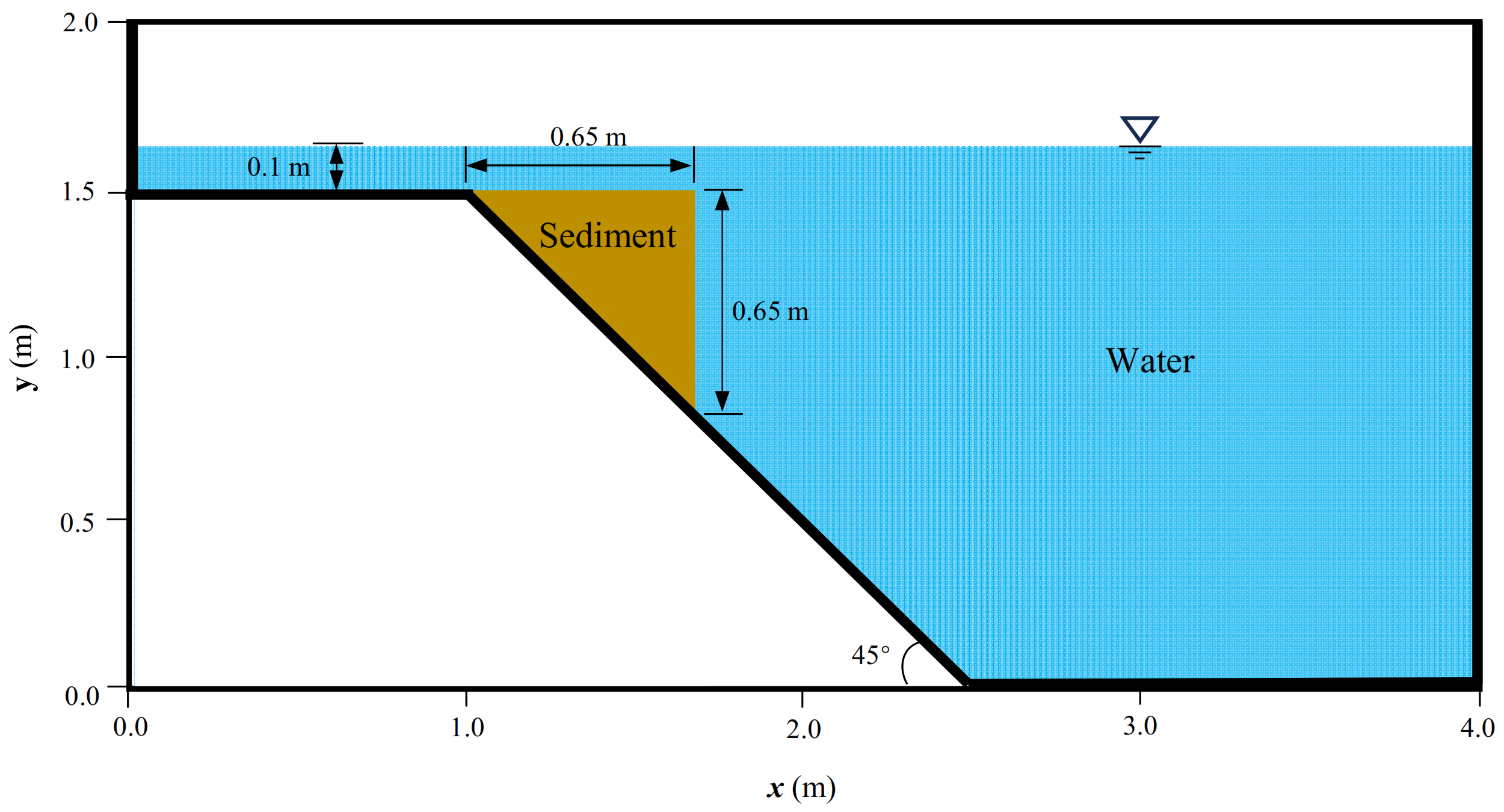
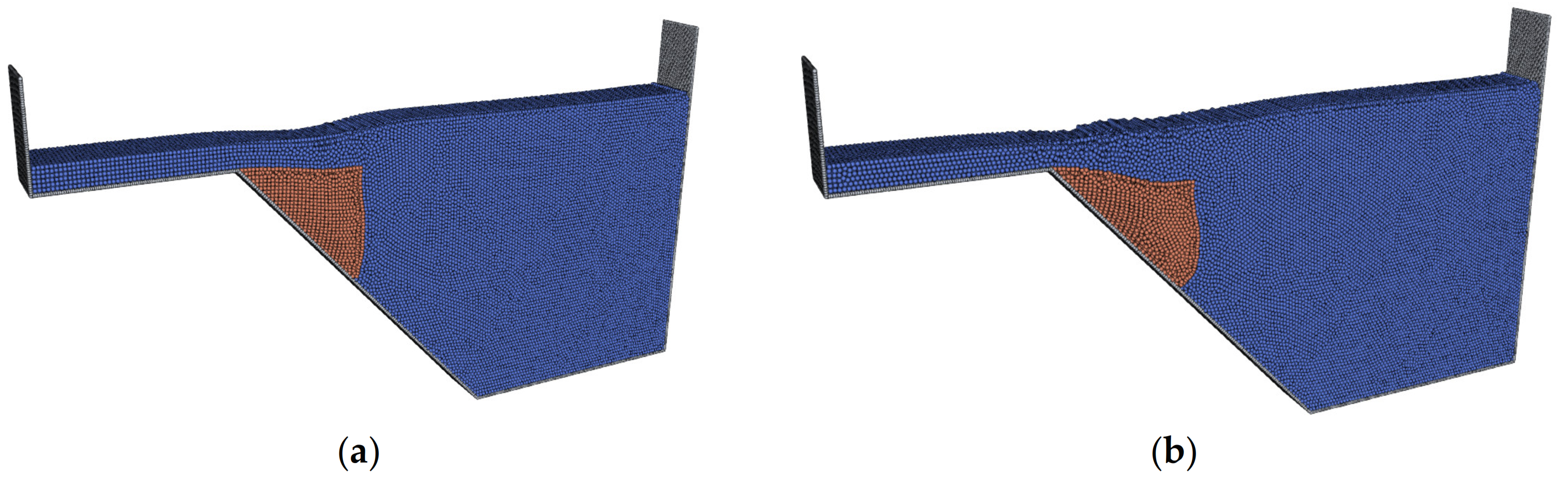
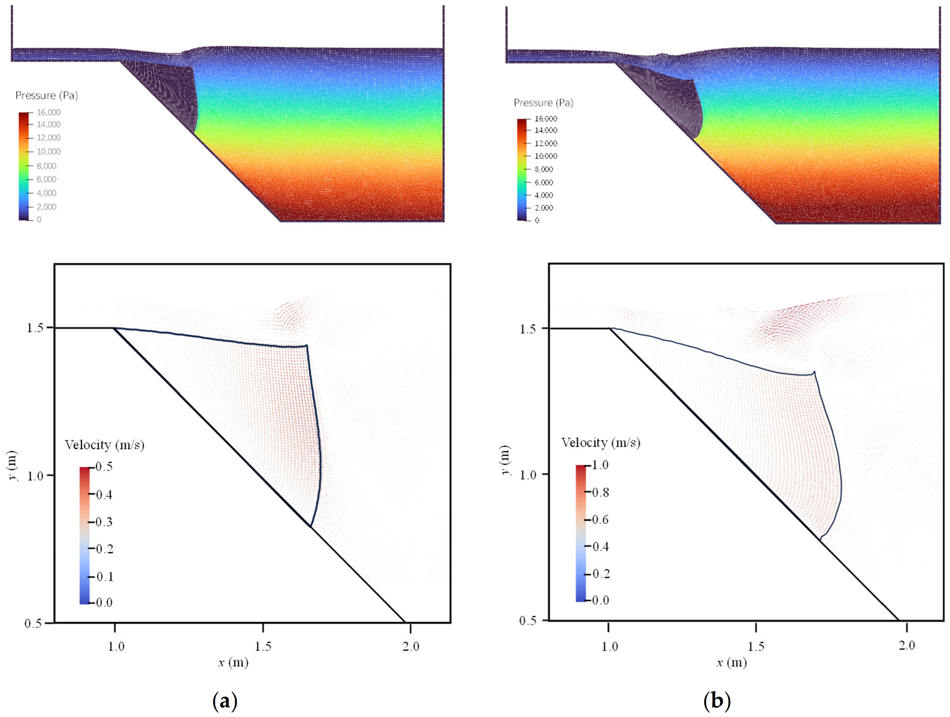
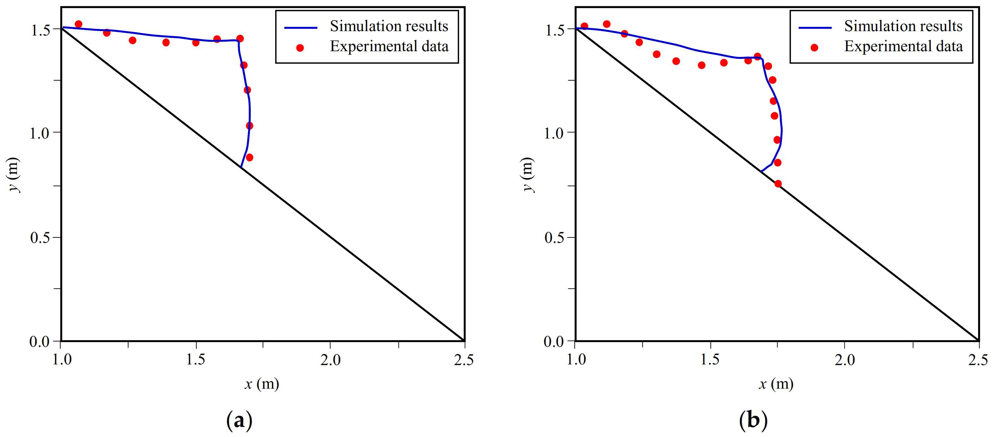
3.1. Benchmark Problem 1: 2D Submarine Landslide Test

To validate the simulation precision of the presented SPH model, a model experiment on the tsunami waves generated by underwater debris flow carried out by Rzadkiewicz et al. [38] is simulated in this section, and the results are compared to the experimental data.

Figure 1 shows the experimental setup, consisting of a rectangular water tank with dimensions of 2.0 m × 4.0 m × 0.3 m. The slope of the inclined bed is set to 45°. In this experiment, the maximum water depth is 1.6 m. Under the effect of gravity, a large amount of sediment (with dimensions of 0.65 m × 0.65 m × 0.30 m) slides down along the 45° slope and generates surge waves.

In

Table 1. Parameters for SPH simulation of underwater debris flow.

Density of sediment	ρs (kg/m3)	1950
Viscosity coefficient of sediment	ηs (Pa·s)	0.15
Yield stress of sediment	τy (Pa)	750
Density of water	ρw (kg/m3)	1000
Viscosity coefficient of water	ηw (Pa·s)	1.0 × 10−3
Gravity acceleration	g (m/s2)	9.8

are the tabulated values of the parameters used in the SPH simulation in this study. The densities of the water and sediment are set to 1000 kg/m³ and 1950 kg/m³, respectively. The viscosity of the water is set to η_w = 0.001 Pa·s. The rheological parameters of the sediment cannot be measured directly in the experiment. According to a trial-and-error approach, we set η_s = 0.15 Pa·s and τ_y = 750 Pa in this study. In this case, the particle spacing D_p = 0.01 m, the smoothing length h = 0.021 m, and the timestep D_t = 1.0 × 10⁻⁴ s.

The SPH model for this experiment consists of approximately 230,000 particles. Based on the SPH simulation, the movement of the underwater slope and the resulting surge waves are obtained. Figure 2 shows the simulated slope configuration and water profile at 0.4 and 0.8 s. Figure 3 shows the simulated water pressure field and the velocity vector of the fluid phase. At t = 0.4 s, the underwater landslide moves downward along the slope, and the water surface at the top of the landslide body collapses to occupy the position of the original landslide body. The maximum velocity of the soil particles is about 0.49 m/s, and the maximum water velocity is about 0.42 m/s. As the collapse of the landslide develops, the maximum velocity of the soil particles reaches 0.87 m/s at t = 0.8 s, and the velocity of the water particles at the right top of the slide is about 0.96 m/s. The relative movement between the landslide and the water is not very significant. The distribution of the water pressure field is obtained, which shows that the pressure in the pure water domain remains almost unchanged during the underwater landslide movement.

To validate the simulation precision of the SPH model, the simulated results are compared to the experimental data recorded in the literature. Figure 4 and Figure 5 show the simulated and tested slope configurations and water profiles at t = 0.4 s and t = 0.8 s, respectively. Through this comparison, it is shown that the simulation results are consistent with the experimental observations.

3.2. Benchmark Problem 2: 3D Submarine Landslide Test

This benchmark problem is based on the 3D physical model experiments on landslide tsunamis carried out by Ataie-Ashtiani and Najafi-Jilani [12]. A 3D SPH modeling is conducted to simulate the landslide movement, and the resulting impulsive waves hereby validate the accuracy and applicability of the SPH model for submarine landslide tsunami modeling.

The experimental setup mainly includes a wave tank with dimensions of 2.5 m × 1.8 m × 25.0 m. A total of 120 experiments were carried out, and the No. 115 case was selected for simulation using the 3D SPH model developed in this work. The cross-section area of the solid block A is 0.0195 m², and the volume V is 0.0039 m³. The special gravity of the sliding granular material γ is 1900 kg/m³, and the total weight W is 7.41 kg. The slope angle of the sliding bed θ is 45°. The water depth in the wave tank h₀ is 0.966 m, and the initial submergence of slide h_c is 0.025 m. A wave gauge was set above the initial position of the slide block. In this simulation, the particle spacing D_p = 0.005 m, the smoothing length h = 0.011 m, and the timestep D_t = 1.0 × 10⁻⁵ s.

Figure 6 shows the simulated sliding process of the confined granular material. Note that the water layer is hidden in the figures in order to display the sediment movement clearly. The maximum velocity is about 0.5 m/s, and the slope configurations at different moments are basically anastomotic with the experimental observations.

Figure 7 shows the propagation of the impulsive waves generated by the underwater landslide. After the initiation of the landslide, the water surface is depressed down at the position near the slide center. The maximum depression of the water surface is about 0.032 m. In front of this depression, a positive wave with a mild crest appears, which propagates along the sliding direction of the granular material. The amplitude of the positive wave is about 0.010 m.

To evaluate the effect of the particle size on the numerical results, the model is discreted into SPH particles with three different sizes (d = 0.005 m, d = 0.010 m, and d = 0.020 m), respectively. Figure 8 shows the time history of the wave amplitude at wave gauge ST1, and compares the simulated results obtained from the model to the different particle sizes. It shows that the simulated wave elevation basically matches the experimental data. When finer particles are used, the simulation results of the SPH model are closer to the experimental data.

The simulation of the above two benchmark problems shows that the numerical results are slightly different from the experimental data. The discrepancies may be due to the size of the SPH particles being much larger than the diameter of the grains, which has some effect on the water–sediment interaction and the evolution of tsunami waves. However, with an increase in particle resolution, this gap is gradually narrowed. Although there are some discrepancies, the numerical results basically match the experimental data, thus, validating the accuracy of the presented SPH model for the simulation of submarine landslide-induced tsunamis.

4. 3D Modeling of Baiyun Submarine Landslide

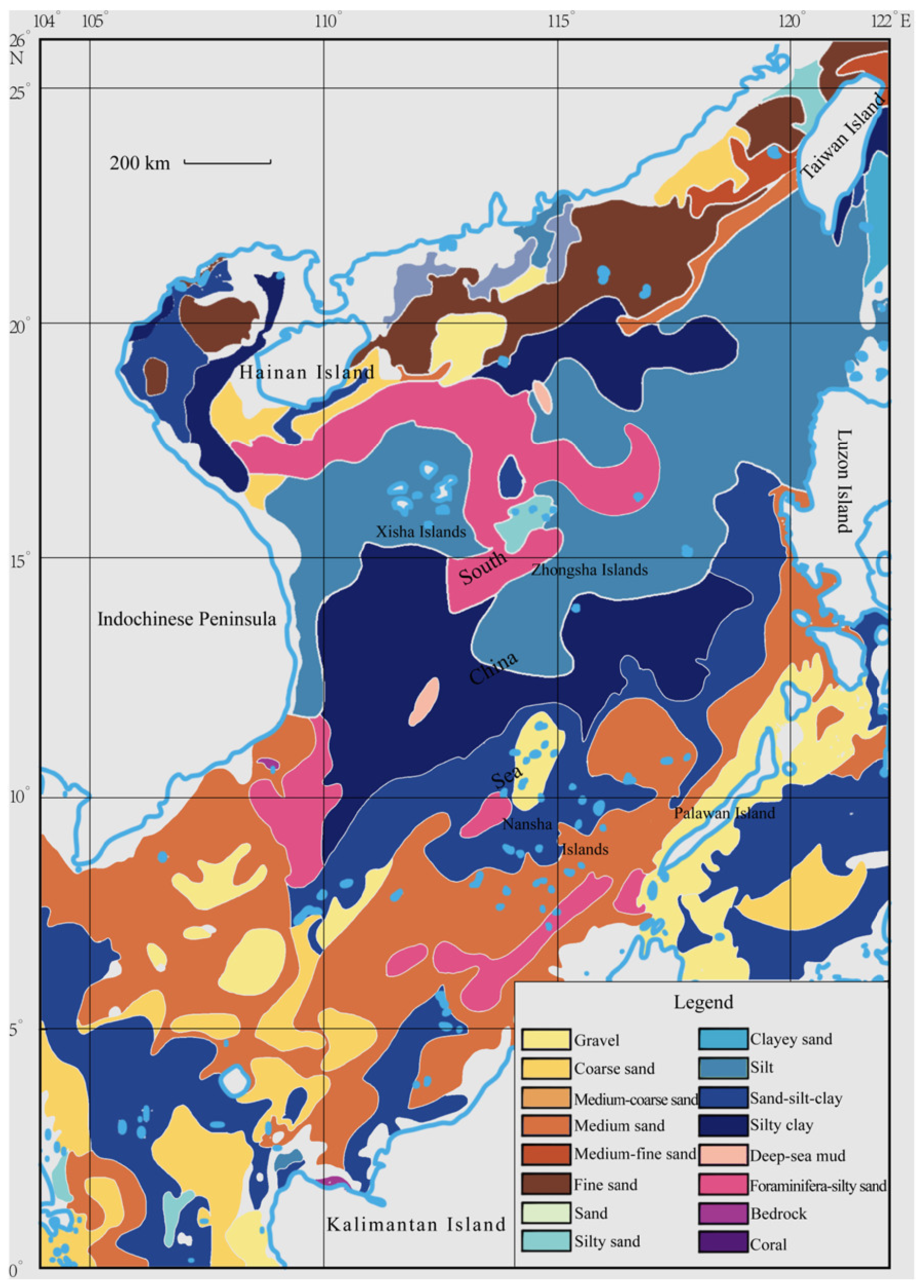
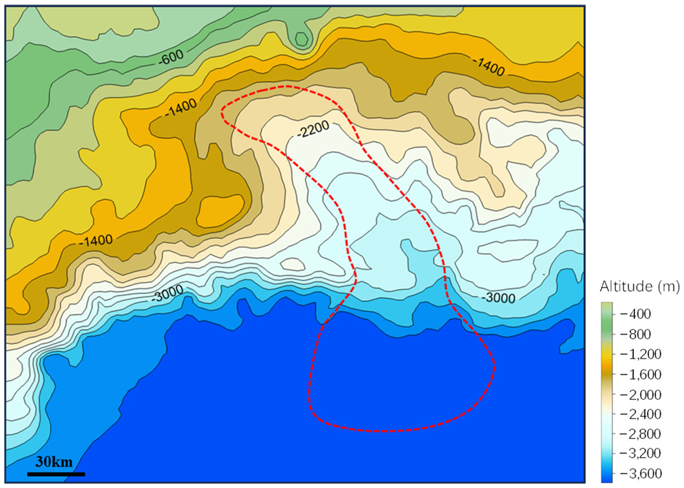
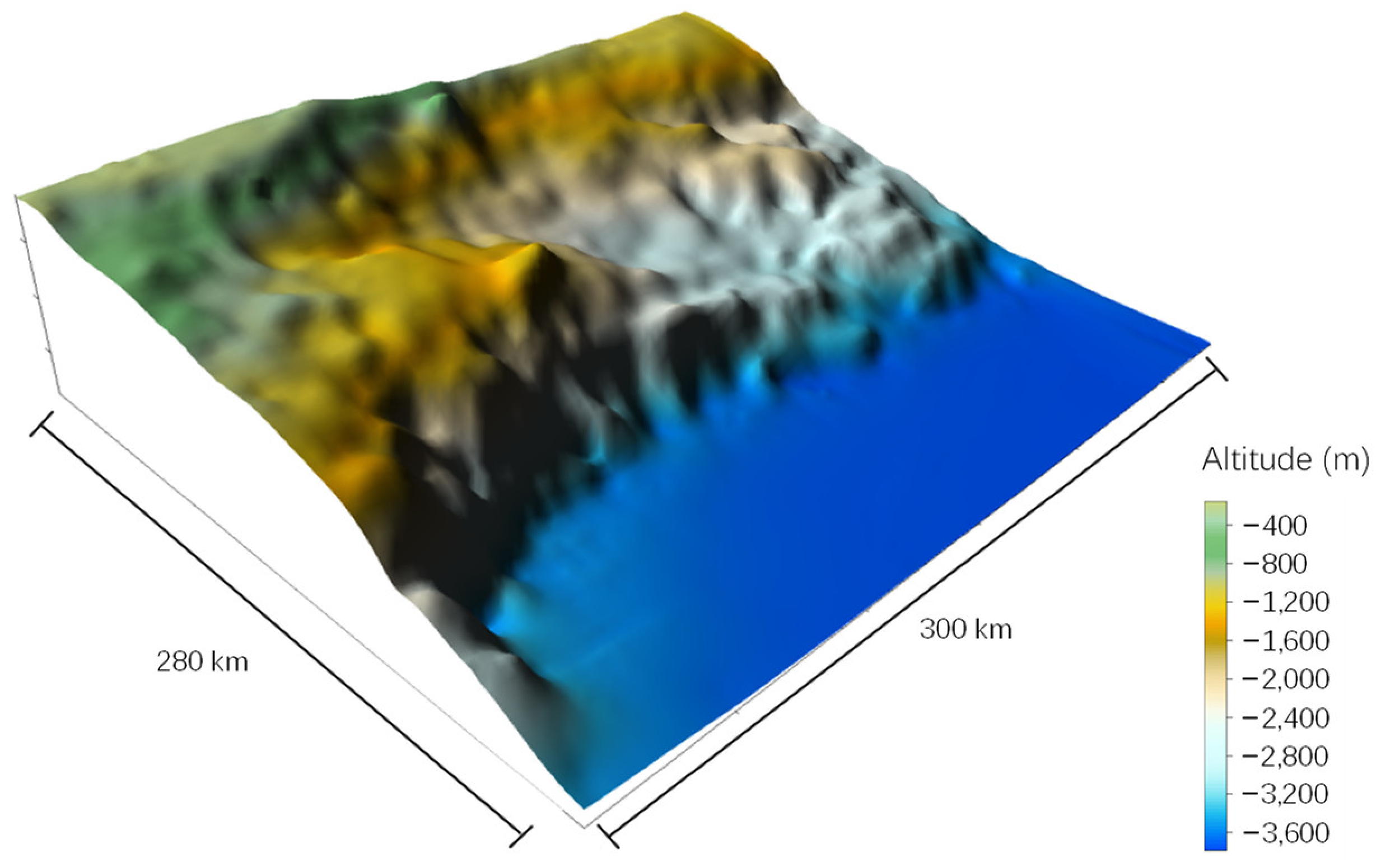
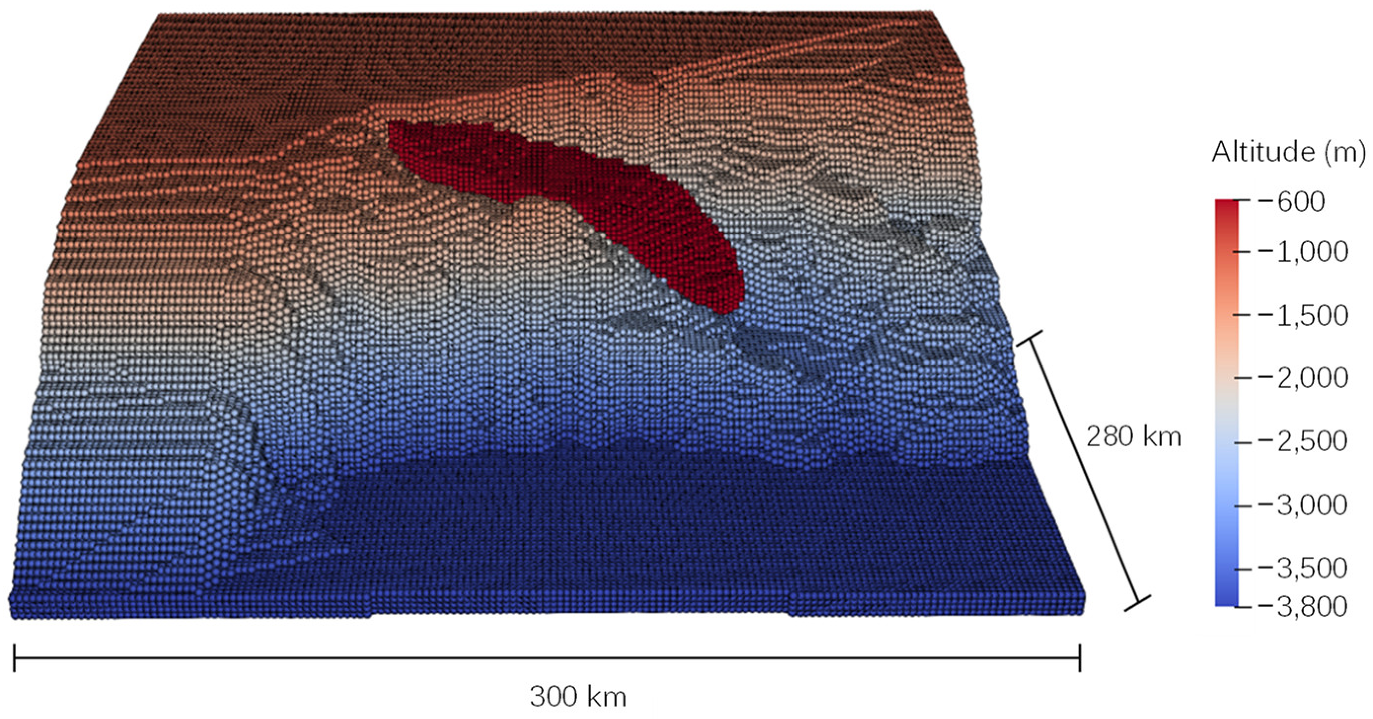
4.1. Baiyun Landslide in the South China Sea

The South China Sea (SCS), surrounded by China, Vietnam, and the Philippines, is the largest marginal sea in the western Pacific Ocean. It receives abundant sediment from river systems, such as the Pearl River, the Red River, and the Mekong River. The distribution of sediment accumulation in the South China Sea is shown in Figure 9 [50]. Additionally, the SCS is in the convergence zone of the Pacific Plate, the Eurasian Plate, and the Indian Plate. Seismic activities are very frequent in this area [51,52,53]. As a result, there are many submarine landslides triggered by earthquakes in the SCS, especially in the Pearl River Mouth Basin (PRMB). According to Zhu et al. [54], more than 142 submarine landslides, with an average area of over 7 km², can be documented in the PRMB. Figure 10 shows the distribution of the seismic faults and submarine landslides, as well as the cities on the coastline of the SCS which have been affected by landslide tsunamis in history. It is reported that the risk of landslide tsunamis is very high in the PRMB [55,56], which poses a great threat to China’s marine construction projects in the SCS. Therefore, it is important to investigate the tsunami characteristics generated by submarine landslides in this area.

The Baiyun landslide is the largest submarine landslide ever found in the deeper part of the PRMB. It was of an enormous magnitude, covering an estimated area of ~5500 km², with a total removal volume of ~1035 km³ of sediment, including a significant amount of mud, gravel, and coral reef blocks [57,58]. The landslide resulted in significant changes to the submarine topography and hydrogeological environment of the SCS, causing severe damage to the marine ecosystem and fisheries resources. It also made a significant impact on China’s maritime security strategy and territorial sovereignty in the SCS. Some previous studies have investigated the tsunamigenic potential of the Baiyun landslide and highlighted the devastating waves generated by the Baiyun landslide [59,60,61]. However, the key features of the landslide propagation and tsunami generation were not reproduced.

4.2. Numerical Simulation of Baiyun Landslide

In this work, the bathymetric DEMs obtained from Ren et al. [62] are used to establish a three-dimensional digital elevation model of the Baiyun landslide area in the PRMB. Figure 11 and Figure 12 show the bathymetric map and the three-dimensional terrain model of the Baiyun landslide in the SCS, respectively.

According to the bathymetric DEMs of the Baiyun landslide, a 3D SPH model of the landslide is established (Figure 13), which includes three different types of particles: boundary particles, landslide body particles, and water particles. In this model, there are over 8.5 million particles with a radius of 50 m. The red particles represent the landslide body, and the color of the boundary particles represents the elevation of the submarine topography, as shown in the legend. To present the submarine terrain clearly, the water particles are hidden in Figure 13. In the SPH model, the density of the water is set to ρ_w = 1000 kg/m³, and the viscosity is set to η_w = 0.001 Pa·s. The landslide body is simulated as a Bingham fluid, with a density of ρ_s = 1860 kg/m³, a viscosity of η_s = 0.15 Pa·s, and a yield stress of τ_y = 750 Pa. To balance the computational efficiency and accuracy, the particle spacing D_p is 50 m in this simulation, h = 1.35 D_p, and D_t = 5.0 × 10⁻² s.

Based on the SPH model, the numerical simulation of the Baiyun submarine landslide motion across the 3D terrain is conducted, and the simulated results are shown in Figure 14. The color of the SPH particles in the figures represents the kinematic velocity of the landslide. Note that the water layer is hidden in the figures in order to clearly observe the propagation behavior of the underwater landslide. The submarine sediment rapidly flows down along the submarine terrain, with a main direction of NW-SE. The maximum velocity is ~40.0 m/s, which occurs about 0.5 h after the landslide’s initiation. The submarine sediment moves downslope and finally spreads out as a fan-shaped planform on the ocean floor, as shown in Figure 14d. The simulated runout distance of the submarine landslide is about 96 km. The whole movement process lasts about 2 h from the initiation to the deposition of the submarine landslide.

The propagation of a submarine landslide disturbs the ambient water and generates surge waves on the sea. Figure 11 shows the simulated water surface elevations above the Baiyun submarine landslide at different moments. According to the simulation results, the movement of the Baiyun submarine landslide could generate large tsunami waves. The amplitude of the leading wave is approximated to be 18.4 m. Figure 15 shows that the propagation of the tsunami wave generated by the Baiyun landslide was in the southeast direction, which basically agrees with the dominant landslide direction, as shown in Figure 14.

4.3. Discussion

Landslide volume and water depth are considered to be two of the most important factors that affect the characteristics of tsunamis generated by landslides [11,12]. However, the Baiyun landslide is an ancient submarine landslide that occurred about 24 M years ago. It is difficult to exactly determine the landslide volume and water depth at that time. Therefore, the effect of the landslide volume and water depth is investigated in this section to predict the potential tsunami generated by the Baiyun landslide.

4.3.1. Effect of Landslide Volume

The volume of the submarine landslide is a significant factor that influences the tsunami waves, which is difficult to precisely measure in situ due to the complex features (bathymetry, etc.) of the marine environment. To investigate the effect of the landslide volume on the tsunami amplitude, SPH simulations of the Baiyun landslide with three different volumes (V₁ = 250 km³, V₂ = 500 km³, and V₃ = 1000 km³) were carried out in this work. Figure 16 shows the tsunami waves at different moments generated by submarine landslides with different volumes. Figure 17 shows the relationship between the tsunami amplitude and the landslide volume. The axis of abscissas represents the maximum height of the head wave generated by the submarine landslide. The axis of ordinates represents the volume of the landslide body. In the simulations, the rheological parameters of the submarine sediment were constant. The simulated results show that the maximum heights of the head waves were about 7.6 m, 15.1 m, and 18.4 m when the landslide volumes were 250 km³, 500 km³, and 1000 km³, respectively. Therefore, it can be concluded that the tsunami amplitude becomes higher as the landslide volume is increased.

The wavelength and period are two important factors with which to evaluate a tsunami disaster. In this study, the effect of the landslide volume on the wavelength and period of the tsunami are investigated according to the 3D SPH numerical simulations. When the landslide volumes are 250 km³, 500 km³, and 1000 km³, the length of the leading waves are about 19.4 km, 22.1 km, and 26.3 km, and the periods range from 24.6 to 28.5 min, respectively. Therefore, it can be concluded that a slide with a larger volume can generate a tsunami with a larger wavelength and lower frequency.

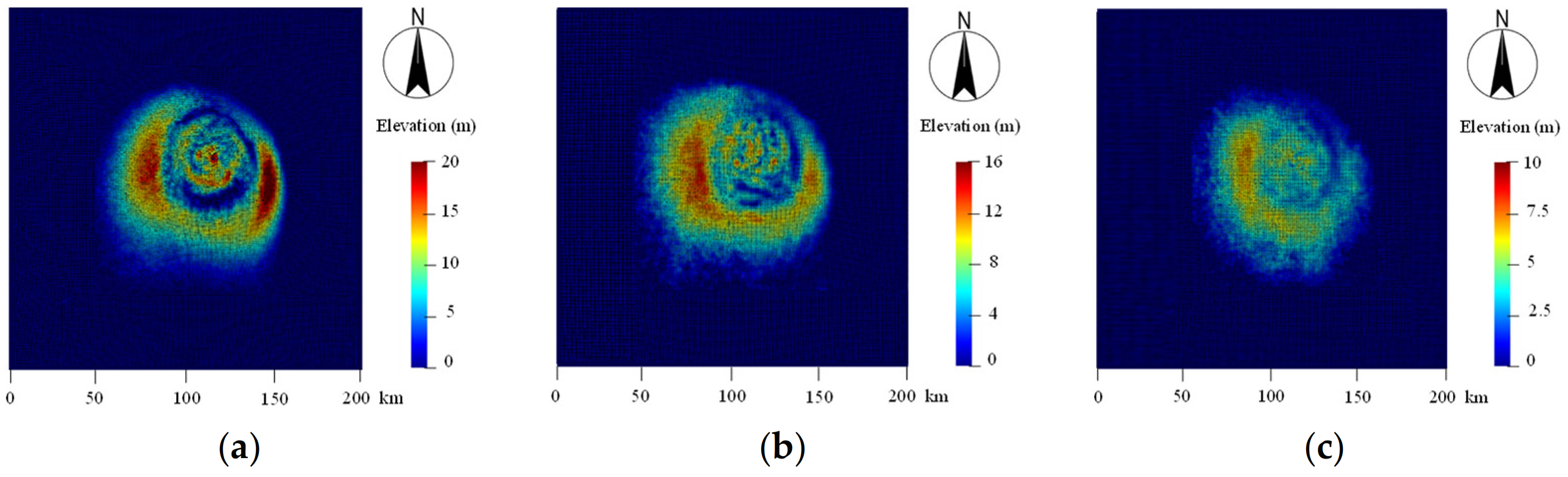
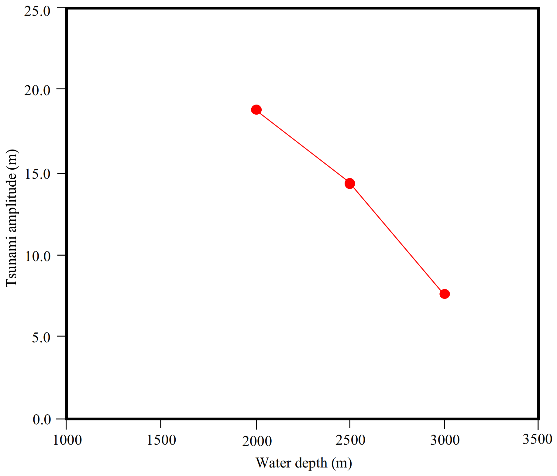
4.3.2. Effect of Water Depth

Submarine landslides usually occur on distinct seabed domains, ranging from shallow coastal areas to the deeper areas of the ocean. According to the bathymetric DEMs, the water depth of the source area of the Baiyun landslide ranged from 2000 m to 3000 m. To investigate the impact of water depth on the tsunami amplitude, simulations of the Baiyun landslide with three different water depths (H₁ = 2000 m, H₂ = 2500 m, and H₃ = 3000 m) of the landslide head scarp are conducted in this work. Figure 18 shows the tsunami waves triggered by the Baiyun landslide (V = 1000 km³) with different water depths at a time of 1.0 h after landslide initiation. The simulation results show that the tsunami amplitude is 18.4 m, 14.5 m, and 7.3 m when the water depth is 2000 m, 2500 m, and 3000 m, respectively. Figure 19 shows the relationship between the tsunami amplitude and water depth, which indicates that a submarine landslide in a shallower water area may result in a larger tsunami.

4.3.3. Limitations of the Presented SPH Model

The 3D SPH model presented in this work can simulate landslide propagation across complex submarine terrain and predict the resulting tsunami waves. In the simulation of the Baiyun landslide, the particle spacing is 50 m, which is much larger than the tsunami wave height. The low resolution may result in considerable errors. However, high-resolution 3D modeling includes millions of SPH particles that greatly reduces the computational efficiency. Therefore, high-efficiency parallel algorithms are necessary to be incorporated into the presented model.

Due to the complex soil–water interaction, the propagation behavior of the sediments is affected by its particle size. In the presented model, the sediment is represented by a series of SPH particles of the same size. The gradation characteristics of the sediment are not considered in the SPH modeling, which may lead to some simulation error.

The simulation results focus on the near-field characteristics of the tsunami waves generated by submarine landslides. Due to the limitations of the presented SPH model, the ocean-basing propagation, run-up behavior, and inundation modeling are not investigated in this work, which are all important for tsunami risk prediction and evaluation.

Therefore, although the simulation results in this work are acceptable, much more attention and effort should be given to break through the above limitations and improve the model’s performance.

5. Conclusions

Submarine landslides play an important role in the generation of tsunami waves and their related hazards. This study presented a three-dimensional SPH model to simulate the propagation of submarine landslides and the resulting tsunami waves. The main conclusions of this work are as follows:

(1)

A 3D numerical model based on the SPH method was established in this work to simulate a submarine landslide’s movement across complex submarine terrain and the near-field characteristics of the resulting tsunami waves.

(2)

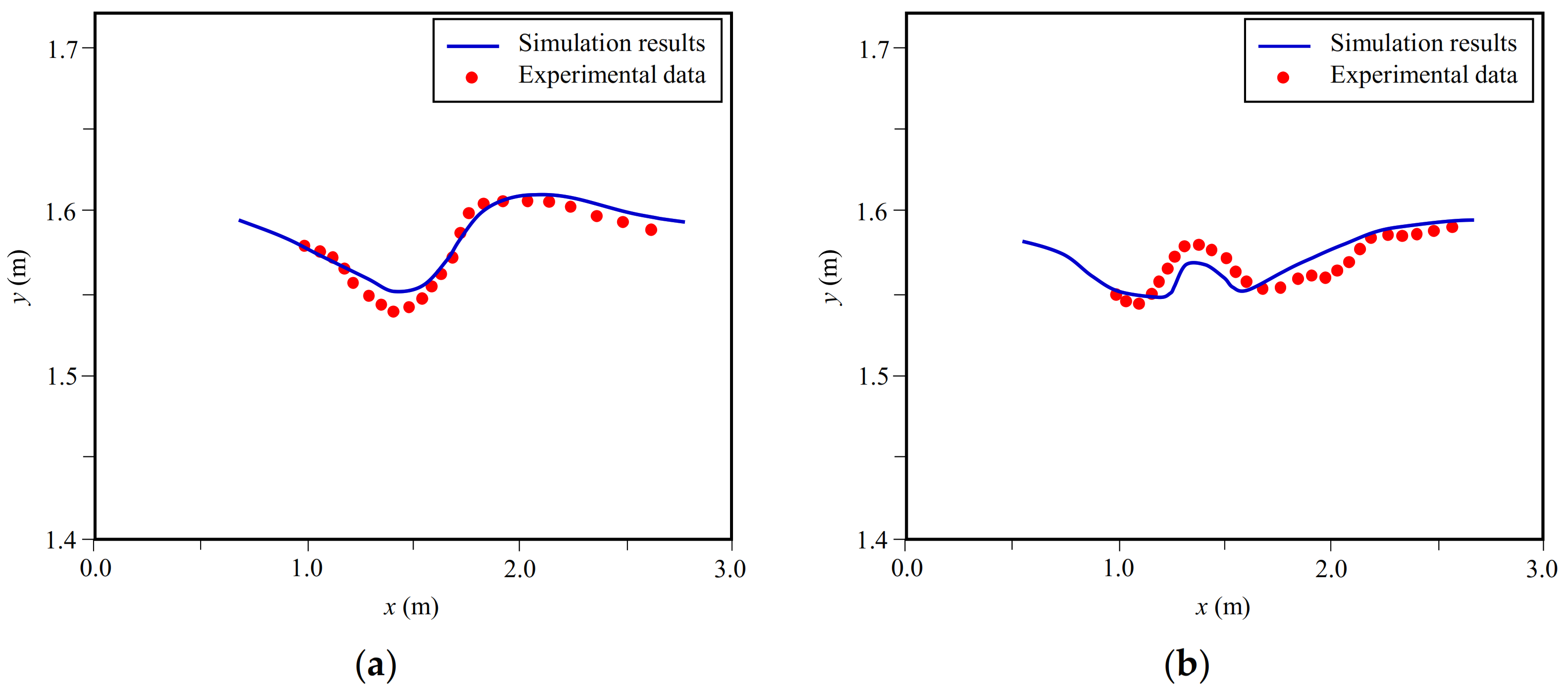
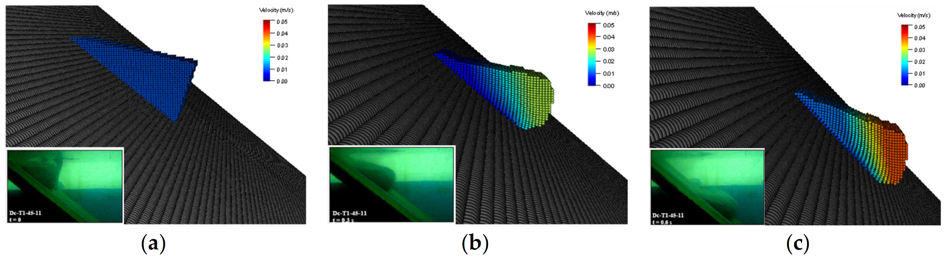
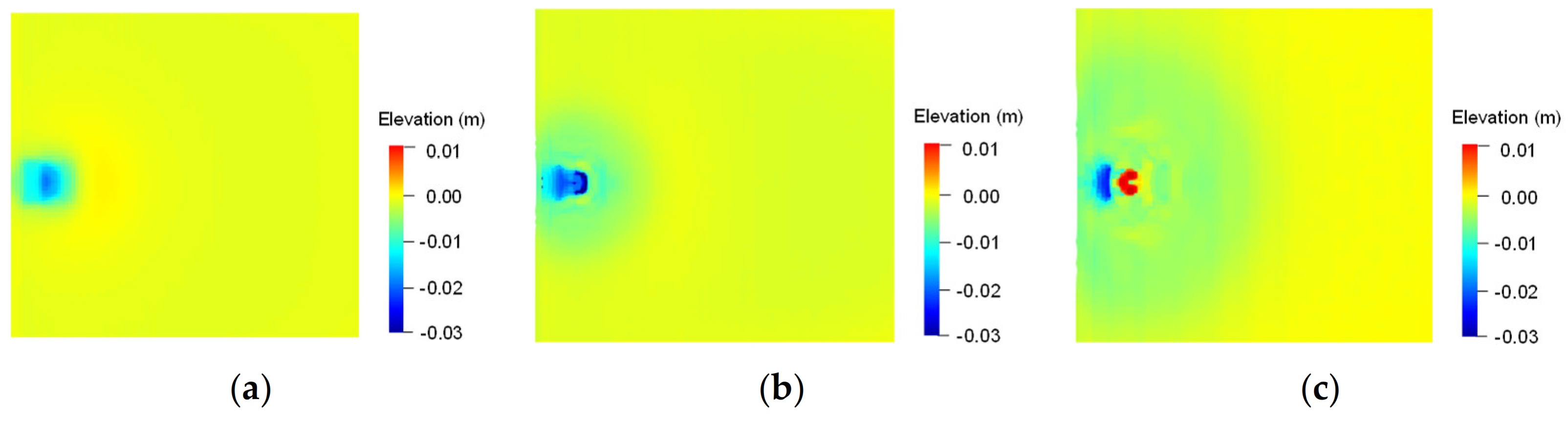
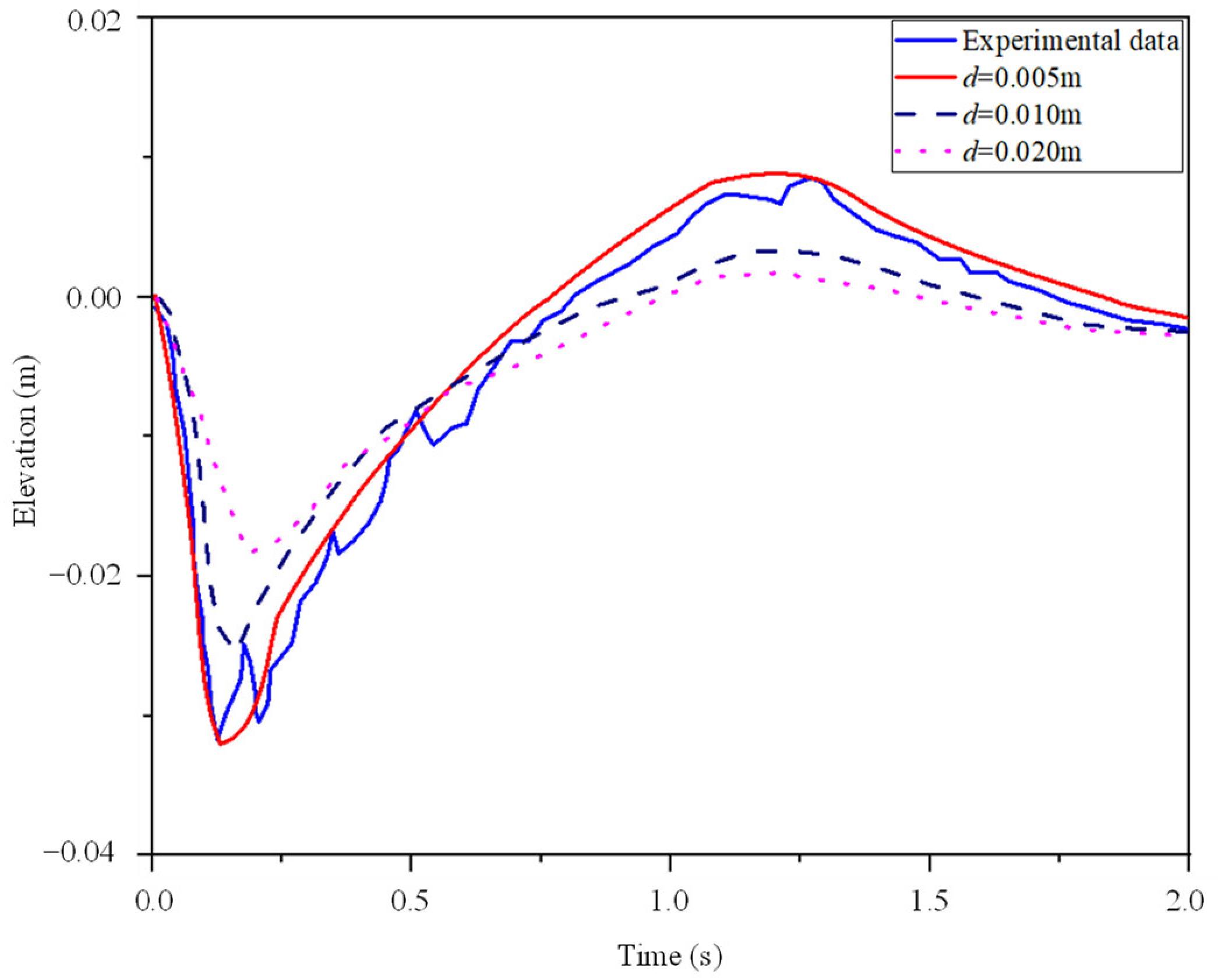
To validate the SPH model, two physical model experiments, in both 2D and 3D, which have been recorded in the literature were simulated and analyzed. The water pressure distribution and velocity vector of the fluid were obtained. The simulated landslide configurations and surface water profiles were compared to the experimental data. The presented results show that despite some discrepancies, the SPH model established in this paper is capable of simulating the soil–water interaction and predicting landslide-generated tsunami events with satisfactory accuracy. The benchmark problem was simulated using the SPH model with different particle resolutions. The results show that the SPH model with finer particle resolution can obtain more accurate results. Therefore, high particle resolutions are necessary in SPH simulations to ensure sufficient computational accuracy.

(3)

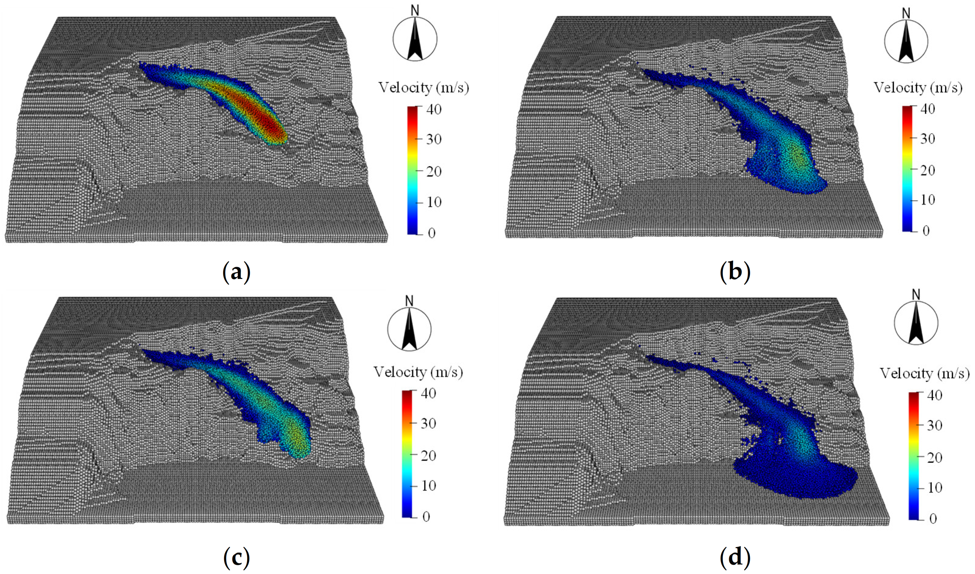
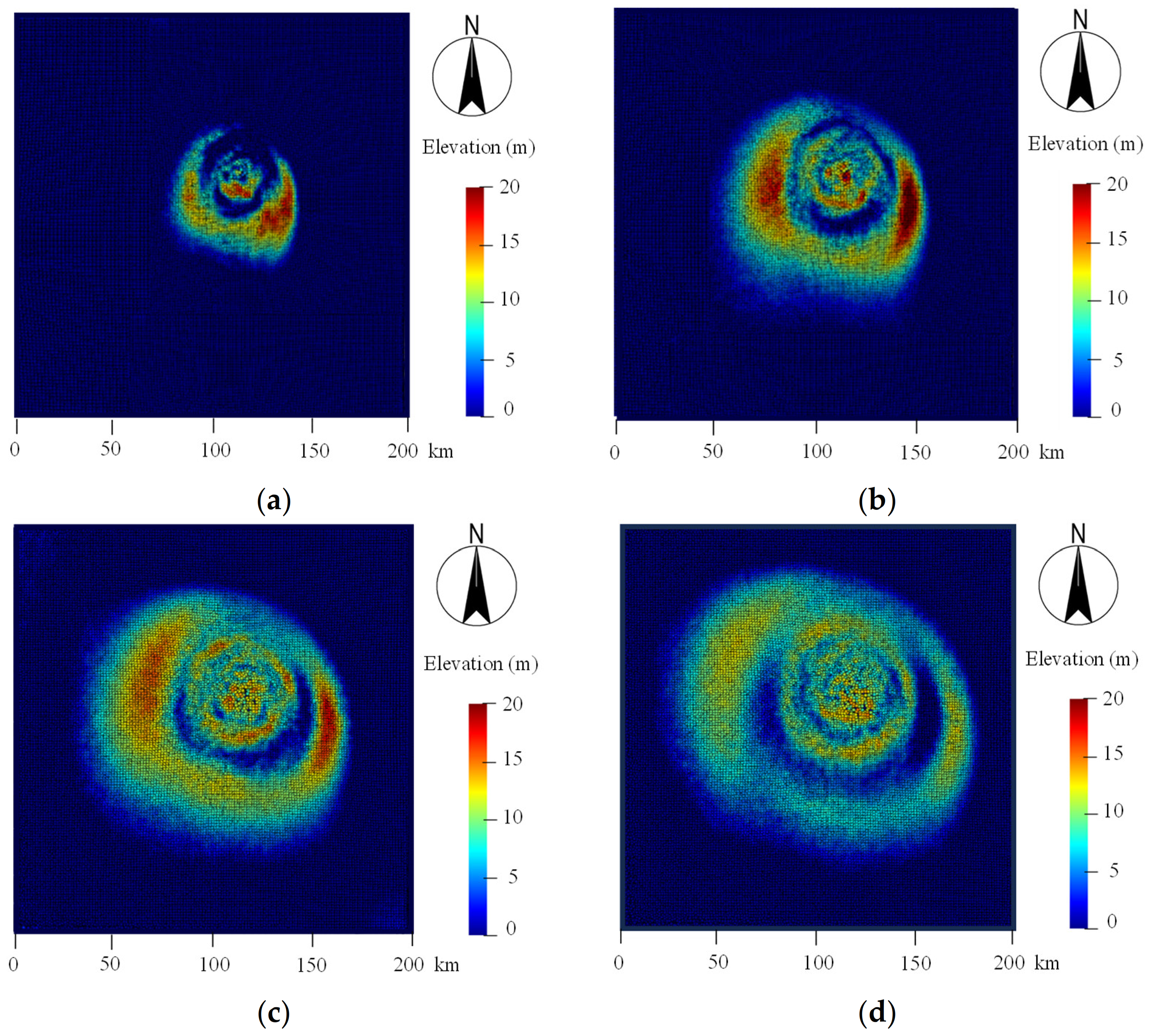
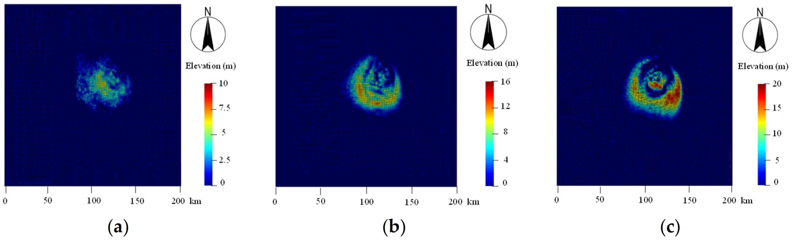
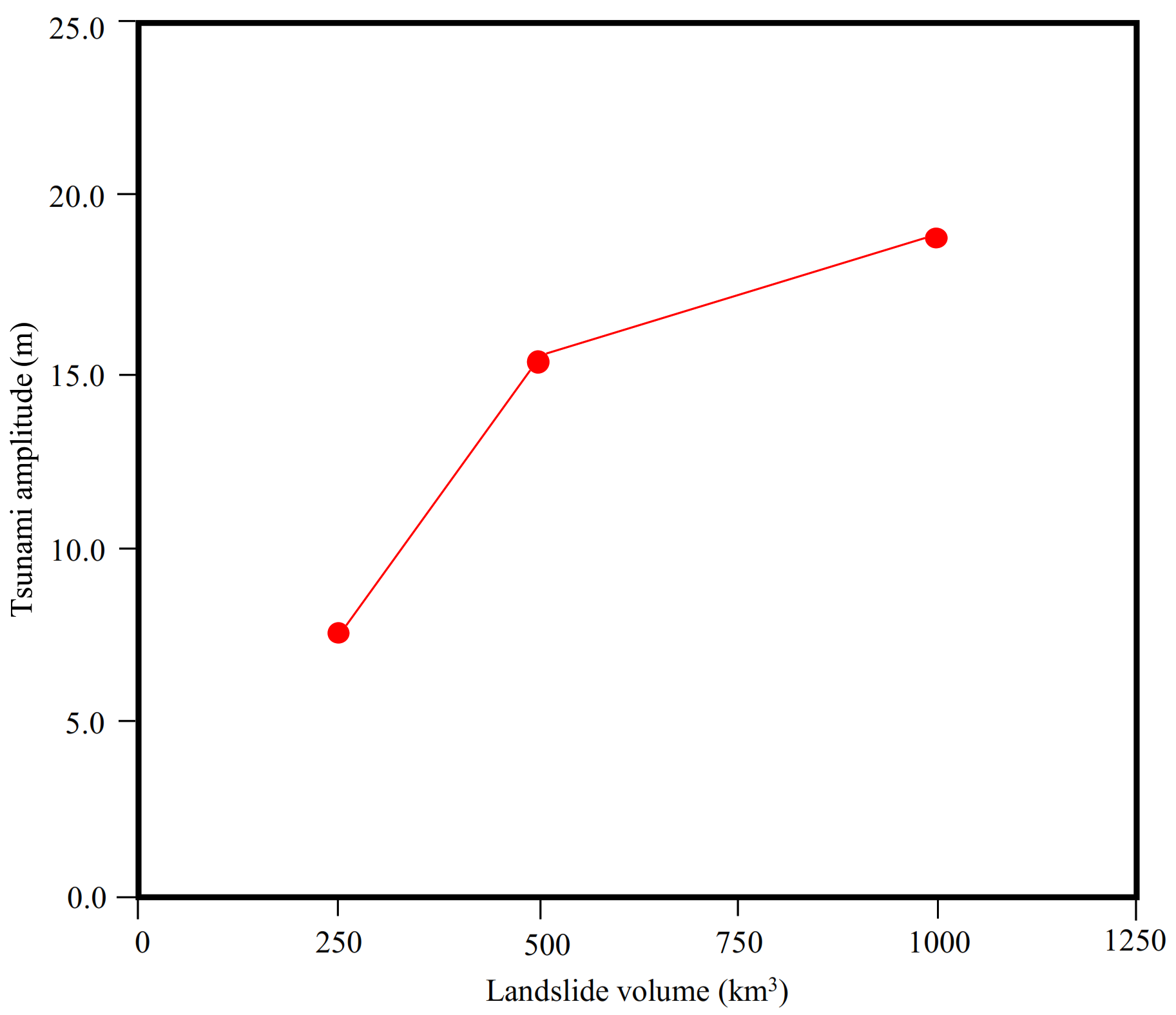
The Baiyun submarine landslide in the South China Sea was simulated using the presented SPH model. The entire motion process of the landslide and the generation of tsunami waves were reproduced. The propagation direction of the leading wave basically agreed with the dominant landslide direction. The effects of water depth and slide volume on the landslide-generated tsunami waves were investigated. The simulation results show that landslides with a larger volume generate larger tsunamis with higher amplitudes, longer wavelengths, and lower frequencies. A landslide in a shallower water area can result in a larger tsunami. These relationships can be used for the rapid prediction of a tsunami disaster.

References

1. Cecioni, C.; Bellotti, G. Modeling tsunamis generated by submerged landslides using depth integrated equations. Appl. Ocean Res. 2010, 32, 343–350. [Google Scholar] [CrossRef]
2. Heller, V.; Spinneken, J. Improved landslide-tsunami prediction: Effects of block model parameters and slide model. J. Geophys. Res. Ocean. 2013, 118, 1489–1507. [Google Scholar] [CrossRef]
3. McAdoo, B.G.; Watts, P. Tsunami hazard from submarine landslides on the Oregon continental slope. Mar. Geol. 2004, 203, 235–245. [Google Scholar] [CrossRef]
4. Harahap, I.S.H.; Huan, V.N.P. Generation, propagation, run-up and impact of landslide triggered tsunami: A literature review. Appl. Mech. Mater. 2014, 567, 724–729. [Google Scholar] [CrossRef]
5. Bondevik, S.; Lovholt, F.; Harbitz, C.; Mangerud, J.; Dawson, A.; Svendsen, J.I. The Storegga Slide tsunami—Comparing field observations with numerical simulations. Mar. Pet. Geol. 2005, 22, 195–208. [Google Scholar] [CrossRef]
6. Fine, I.V.; Rabinovich, A.B.; Bornhold, B.D.; Thomson, R.E.; Kulikov, E.A. The Grand Banks landslide-generated tsunami of November 18, 1929: Preliminary analysis and numerical modeling. Mar. Geol. 2005, 215, 45–57. [Google Scholar] [CrossRef]
7. Tanioka, Y. Analysis of the far-field tsunamis generated by the 1998 Papua New Guinea earthquake. Geophys. Res. Lett. 1999, 26, 3393–3396. [Google Scholar] [CrossRef]
8. Fornaciai, A.; Favalli, M.; Nannipieri, L. Numerical simulation of the tsunamis generated by the Sciara del Fuoco landslides (Stromboli Island, Italy). Sci. Rep. 2019, 9, 18542. [Google Scholar] [CrossRef]
9. Sassa, S.; Takagawa, T. Liquefied gravity flow-induced tsunami: First evidence and comparison from the 2018 Indonesia Sulawesi earthquake and tsunami disasters. Landslides 2019, 16, 195–200. [Google Scholar] [CrossRef]
10. Watts, P. Wavemaker curves for tsunamis generated by underwater landslides. J. Waterw. Port Coast. Ocean Eng. 1998, 124, 127–137. [Google Scholar] [CrossRef]
11. Watts, P. Tsunami features of solid block underwater landslides. J. Waterw. Port Coast. Ocean Eng. 2000, 126, 144–152. [Google Scholar] [CrossRef]
12. Ataie-Ashtiani, B.; Najafi-Jilani, A. Laboratory investigations on impulsive waves caused by underwater landslide. Coast. Eng. 2008, 55, 989–1004. [Google Scholar] [CrossRef]
13. Hu, Y.X.; Li, H.B.; Li, C.J.; Zhou, J.W. Quantitative evaluation in classification and amplitude of near-field landslide generated wave induced by granular debris. Ocean Eng. 2022, 261, 112142. [Google Scholar] [CrossRef]
14. Bregoli, F.; Bateman, A.; Medina, V. Tsunamis generated by fast granular landslides: 3D experiments and empirical predictors. J. Hydraul. Res. 2017, 55, 743–758. [Google Scholar] [CrossRef]
15. Rauter, M.; Hoße, L.; Mulligan, R.P.; Take, W.A.; Løvholt, F. Numerical simulation of impulse wave generation by idealized landslides with OpenFOAM. Coast. Eng. 2020, 165, 103815. [Google Scholar] [CrossRef]
16. Deng, X.; He, S.; Cao, Z.; Wu, T. Numerical investigation of the hydrodynamic response of an impermeable sea-wall subjected to artificial submarine landslide-induced tsunamis. Landslides 2021, 18, 3937–3952. [Google Scholar]
17. Yavari-Ramshe, S.; Ataie-Ashtiani, B. A rigorous finite volume model to simulate subaerial and submarine landslide-generated waves. Landslides 2015, 14, 203–221. [Google Scholar] [CrossRef]
18. Fu, L.; Jin, Y.C. Investigation of non-deformable and deformable landslides using meshfree method. Ocean Eng. 2015, 109, 192–206. [Google Scholar] [CrossRef]
19. Zhao, K.L.; Qiu, L.C.; Liu, Y. Two-layer two-phase material point method simulation of granular landslides and generated tsunami waves. Phys. Fluids 2022, 34, 123312. [Google Scholar] [CrossRef]
20. Mulligan, R.; Franci, A.; Celigueta, M.; Take, W. Simulations of landslide wave generation and propagation using the particle finite element method. J. Geophys. Res. Ocean. 2020, 125, e2019JC015873. [Google Scholar] [CrossRef]
21. Qiu, L.C.; Tian, L.; Liu, X.; Han, Y. A 3D multiple-relaxation-time LBM for modeling landslide-induced tsunami waves. Eng. Anal. Bound. Elem. 2019, 102, 51–59. [Google Scholar] [CrossRef]
22. Yavari-Ramshe, S.; Ataie-Ashtiani, B. Numerical modeling of subaerial and submarine landslide-generated tsunami waves—Recent advances and future challenges. Landslides 2016, 13, 1325–1368. [Google Scholar] [CrossRef]
23. Altomare, C.; Scandura, P.; Cáceres, I.; Viccione, G. Large-scale wave breaking over a barred beach: SPH numerical simulation and comparison with experiments. Coast. Eng. 2023, 185, 104362. [Google Scholar] [CrossRef]
24. De Padova, D.; Ben Meftah, M.; De Serio, F.; Mossa, M.; Sibilla, S. Characteristics of breaking vorticity in spilling and plunging waves investigated numerically by SPH. Environ. Fluid Mech. 2020, 20, 233–260. [Google Scholar] [CrossRef]
25. Lowe, R.J.; Buckley, M.L.; Altomare, C.; Rijnsdorp, D.P.; Yao, Y.; Suzuki, T.; Bricker, J.D. Numerical simulations of surf zone wave dynamics using Smoothed Particle Hydrodynamics. Ocean Model. 2019, 144, 101481. [Google Scholar] [CrossRef]
26. Lowe, R.J.; Altomare, C.; Buckley, M.L.; da Silva, R.F.; Hansen, J.E.; Rijnsdorp, D.P.; Domínguez, J.M.; Crespo, A.J.C. Smoothed Particle Hydrodynamics simulations of reef surf zone processes driven by plunging irregular waves. Ocean Model. 2022, 171, 101945. [Google Scholar] [CrossRef]
27. Makris, C.V.; Memos, C.D.; Krestenitis, Y.N. Numerical modeling of surf zone dynamics under weakly plunging breakers with SPH method. Ocean Model. 2016, 98, 12–35. [Google Scholar] [CrossRef]
28. Roselli, R.A.R.; Vernengo, G.; Brizzolara, S.; Guercio, R. SPH simulation of periodic wave breaking in the surf zone-A detailed fluid dynamic validation. Ocean Eng. 2019, 176, 20–30. [Google Scholar] [CrossRef]
29. Dai, Z.L.; Xie, J.W.; Jiang, M.T. A coupled peridynamics–smoothed particle hydrodynamics model for fracture analysis of fluid–structure interactions. Ocean Eng. 2023, 279, 114582. [Google Scholar] [CrossRef]
30. Capone, T.; Panizzo, A.; Monaghan, J.J. SPH modelling of water waves generated by submarine landslides. J. Hydraul. Res. 2010, 48, 80–84. [Google Scholar] [CrossRef]
31. Shi, C.; An, Y.; Wu, Q.; Liu, Q.; Cao, Z. Numerical simulation of landslide-generated waves using a soil-water coupling smoothed particle hydrodynamics model. Adv. Water Resour. 2016, 92, 130–141. [Google Scholar] [CrossRef]
32. Farhadi, A. ISPH numerical simulation of tsunami generation by submarine landslides. Arab. J. Geosci. 2018, 11, 330. [Google Scholar] [CrossRef]
33. Mahallem, A.; Roudane, M.; Krimi, A.; Gouri, S.A. Smoothed Particle Hydrodynamics for modelling landslide-water interaction problems. Landslides 2022, 19, 1249–1263. [Google Scholar] [CrossRef]
34. Bu, S.; Li, D.; Chen, S.; Xiao, C.; Li, Y. Numerical simulation of landslide generated waves using a SPH-DEM coupling model. Ocean Eng. 2022, 258, 111826. [Google Scholar] [CrossRef]
35. Tan, H.; Xu, Q.; Chen, S. Subaerial rigid landslide-tsunamis: Insights from a block DEM-SPH model. Eng. Anal. Bound. Elem. 2018, 95, 297–314. [Google Scholar] [CrossRef]
36. Hu, Y.X.; Zhu, Y.G.; Li, H.B.; Li, C.J.; Zhou, J.W. Numerical estimation of landslide-generated waves at Kaiding Slopes, Houziyan Reservior, China, using a coupled DEM-SPH method. Landslides 2021, 18, 3435–3448. [Google Scholar] [CrossRef]
37. Xu, W.J.; Yao, Z.G.; Luo, Y.T.; Dong, X.Y. Study on landslide-induced wave disasters using a 3D coupled SPH-DEM method. Bull. Eng. Geol. Environ. 2020, 79, 467–483. [Google Scholar] [CrossRef]
38. Rzadkiewicz, S.A.; Mariotti, C.; Heinrich, P. Numerical simulation of submarine landslides and their hydraulic effects. J. Waterw. Port Coast. Ocean Eng. 1997, 123, 149–157. [Google Scholar] [CrossRef]
39. Lucy, L.B. A numerical approach to the testing of the fission hypothesis. Astron. J. 1977, 82, 1013–1024. [Google Scholar] [CrossRef]
40. Liu, M.B.; Liu, G. Smoothed particle hydrodynamics (SPH): An overview and recent developments. Arch. Comput. Methods Eng. 2020, 17, 25–76. [Google Scholar] [CrossRef]
41. Swegle, J.W.; Hicks, D.L.; Attaway, S.W. Smoothed particle hydrodynamics stability analysis. J. Comput. Phys. 1995, 116, 123–134. [Google Scholar] [CrossRef]
42. Wendland, H. Piecewise polynomial, positive definite and compactly supported radial functions of minimal degree. Adv. Comput. Math. 1995, 4, 389–396. [Google Scholar] [CrossRef]
43. Lo, E.Y.M.; Shao, S. Simulation of near-shore solitary wave mechanics by an incompressible SPH method. Appl. Ocean Res. 2002, 24, 275–286. [Google Scholar]
44. Dalrymple, R.A.; Rogers, B.D. Numerical modeling of water waves with the SPH method. Coast. Eng. 2006, 53, 141–147. [Google Scholar] [CrossRef]
45. Hu, X.Y.; Adams, N.A. An incompressible multi-phase SPH method. J. Comput. Phys. 2007, 227, 264–278. [Google Scholar] [CrossRef]
46. Adami, S.; Hu, X.Y.; Adams, N.A. A new surface-tension formulation for multi-phase SPH using a reproducing divergence approximation. J. Comput. Phys. 2010, 229, 5011–5021. [Google Scholar] [CrossRef]
47. Dai, Z.L.; Huang, Y.; Cheng, H.L.; Xu, Q. SPH model for fluid–structure interaction and its application to debris flow impact estimation. Landslides 2017, 14, 917–928. [Google Scholar] [CrossRef]
48. Dai, Z.L.; Huang, Y.; Cheng, H.L.; Xu, Q. 3D numerical modeling using smoothed particle hydrodynamics of flow-like landslide propagation triggered by the 2008 Wenchuan earthquake. Eng. Geol. 2014, 180, 21–33. [Google Scholar] [CrossRef]
49. Dai, Z.; Xie, J.; Qin, S.; Chen, S. Numerical investigation of surge waves generated by submarine debris flows. Water 2021, 13, 2276. [Google Scholar] [CrossRef]
50. Ye, Y.C. Marine Hazardous Geology of China; Maritime Press: Beijing, China, 2012. [Google Scholar]
51. Megawati, K.; Shaw, F.; Sieh, K.; Huang, Z.H.; Wu, T.R.; Lin, Y.N.; Tan, S.K.; Pan, T.C. Tsunami hazard from the subduction megathrust of the South China Sea: Part I. Source characterization and the resulting tsunami. J. Asian Earth Sci. 2009, 36, 13–20. [Google Scholar] [CrossRef]
52. Mardi, N.H.; Malek, M.A.; Liew, M.S. Tsunami simulation due to seaquake at Manila Trench and Sulu Trench. Nat. Hazards 2017, 85, 1723–1741. [Google Scholar] [CrossRef]
53. Xu, Z.G.; Liang, S.S.; Rahman, M.N.B.; Li, H.W.; Shi, J.Y. Historical earthquakes, tsunamis and real-time earthquake monitoring for tsunami advisory in the South China Sea region. Nat. Hazards 2021, 107, 771–793. [Google Scholar] [CrossRef]
54. Zhu, C.Q.; Cheng, S.; Li, Q.P.; Shan, H.X.; Lu, J.A.; Shen, Z.C.; Liu, X.L.; Jia, Y.G. Giant Submarine Landslide in the South China Sea: Evidence, Causes, and Implications. J. Mar. Sci. Eng. 2019, 7, 152. [Google Scholar] [CrossRef]
55. Li, L.L.; Qiu, Q.; Li, Z.G.; Zhang, P.Z. Tsunami hazard assessment in the South China Sea: A review of recent progress and research gaps. Sci. China-Earth Sci. 2022, 65, 783–809. [Google Scholar] [CrossRef]
56. Pan, X.Y.; Li, L.L.; Nguyen, H.P.; Wang, D.W.; Switzer, A.D. Submarine Landslides in the West Continental Slope of the South China Sea and Their Tsunamigenic Potential. Front. Earth Sci. 2022, 10, 843173. [Google Scholar] [CrossRef]
57. Sun, Q.; Xie, X.; Piper, D.J.W.; Wu, J.; Wu, S. Three dimensional seismic anatomy of multi-stage mass transport deposits in the Pearl River Mouth Basin, northern South China Sea: Their ages and kinematics. Mar. Geol. 2017, 393, 93–108. [Google Scholar] [CrossRef]
58. Sun, Q.; Cartwright, J.; Xie, X.; Lu, X.; Yuan, S.; Chen, C. Reconstruction of repeated Quaternary slope failures in the northern South China Sea. Mar. Geol. 2018, 401, 17–35. [Google Scholar] [CrossRef]
59. Sun, Y.; Huang, B. A potential tsunami impact assessment of submarine landslide at Baiyun Depression in Northern South China Sea. Geoenviron. Disasters 2014, 1, 7. [Google Scholar]
60. Ren, Z.; Zhao, X.; Liu, H. Numerical study of the landslide tsunami in the South China Sea using Herschel-Bulkley rheological theory. Phys. Fluids 2019, 31, 056601. [Google Scholar] [CrossRef]
61. Li, L.L.; Shi, F.Y.; Ma, G.F.; Qiu, Q. Tsunamigenic potential of the Baiyun Slide complex in the South China Sea. J. Geophys. Res. Solid Earth 2019, 124, 7680–7698. [Google Scholar] [CrossRef]
62. Ren, Z.Y.; Liu, H.; Li, L.L.; Wang, Y.C.; Sun, Q.L. On the effects of rheological behavior on landslide motion and tsunami hazard for the Baiyun Slide in the South China Sea. Landslides 2023, 20, 1599–1616. [Google Scholar] [CrossRef]
Figure 1. Schematic of the experimental setup of the underwater debris flow.
Jmse 11 02015 g001
Figure 2. Simulated slope configuration and water profile at different moments. (a) t = 0.4 s and (b) t = 0.8 s.
Jmse 11 02015 g002
Figure 3. Simulated water pressure field (first row) and velocity vector of fluid phase (second row) at (a) t = 0.4 s and (b) t = 0.8 s.
Jmse 11 02015 g003
Figure 4. Comparison of the simulated and tested slope configurations at different times. (a) t = 0.4 s and (b) t = 0.8 s.
Jmse 11 02015 g004
Figure 5. Comparison of simulated and recorded water profiles at different times. (a) t = 0.4 s and (b) t = 0.8 s.
Jmse 11 02015 g005
Figure 6. Simulated slope configuration at different moments. (a) t = 0.0 s, (b) t = 0.3 s, and (c) t = 0.6 s. The experimental scenarios in the figures are from reference [12].
Jmse 11 02015 g006
Figure 7. Simulated slope configuration at different moments. (a) t = 0.1 s, (b) t = 0.3 s, and (c) t = 1.2 s.
Jmse 11 02015 g007
Figure 8. Recorded and simulated time history of wave amplitude at wave gauge ST1.
Jmse 11 02015 g008
Figure 9. Distribution of sediment accumulation in the South China Sea [50].
Jmse 11 02015 g009
Figure 10. Distribution of faults, submarine landslides, and cities effected by the tsunami around the South China Sea.
Jmse 11 02015 g010
Figure 11. Bathymetric map of Baiyun landslide in the SCS.
Jmse 11 02015 g011
Figure 12. Three-dimensional terrain model of Baiyun landslide.
Jmse 11 02015 g012
Figure 13. A 3D SPH model of the Baiyun submarine landslide.
Jmse 11 02015 g013
Figure 14. The 3D simulated results for the motion process of the Baiyun submarine landslide. (a) t = 0.5 h, (b) t = 1.0 h, (c) t = 1.5 h, and (d) t = 2.0 h.
Jmse 11 02015 g014
Figure 15. Tsunami waves triggered by the Baiyun landslide at different moments. (a) t = 0.5 h, (b) t = 1.0 h, (c) t = 1.5 h, and (d) t = 2.0 h.
Jmse 11 02015 g015
Figure 16. Tsunami waves triggered by Baiyun landslides with different volumes. (a) V = 250 km3, (b) V = 500 km3, and (c) V = 1000 km3.
Jmse 11 02015 g016
Figure 17. Relationship between the tsunami amplitude and the landslide volume.
Jmse 11 02015 g017
Figure 18. Tsunami waves triggered by Baiyun landslides with different water depths. (a) H1 = 2000 m, (b) H2 = 2500 m, and (c) H3 = 3000 m.
Jmse 11 02015 g018
Figure 19. Relationship between the tsunami amplitude and water depth.
Jmse 11 02015 g019