
A K-Nearest Neighbors Algorithm in Python for Visualizing the 3D Stratigraphic Architecture of the Llobregat River Delta in NE Spain


Abstract
:1. Introduction
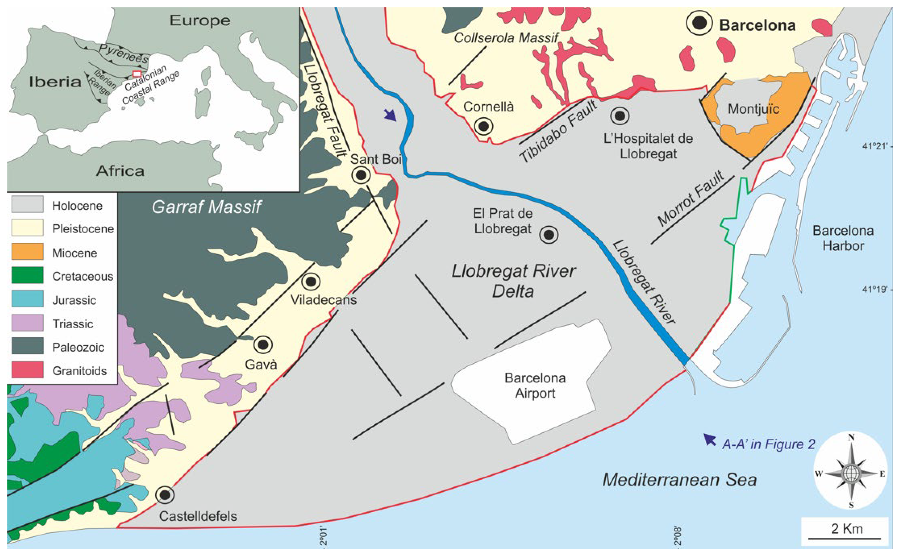
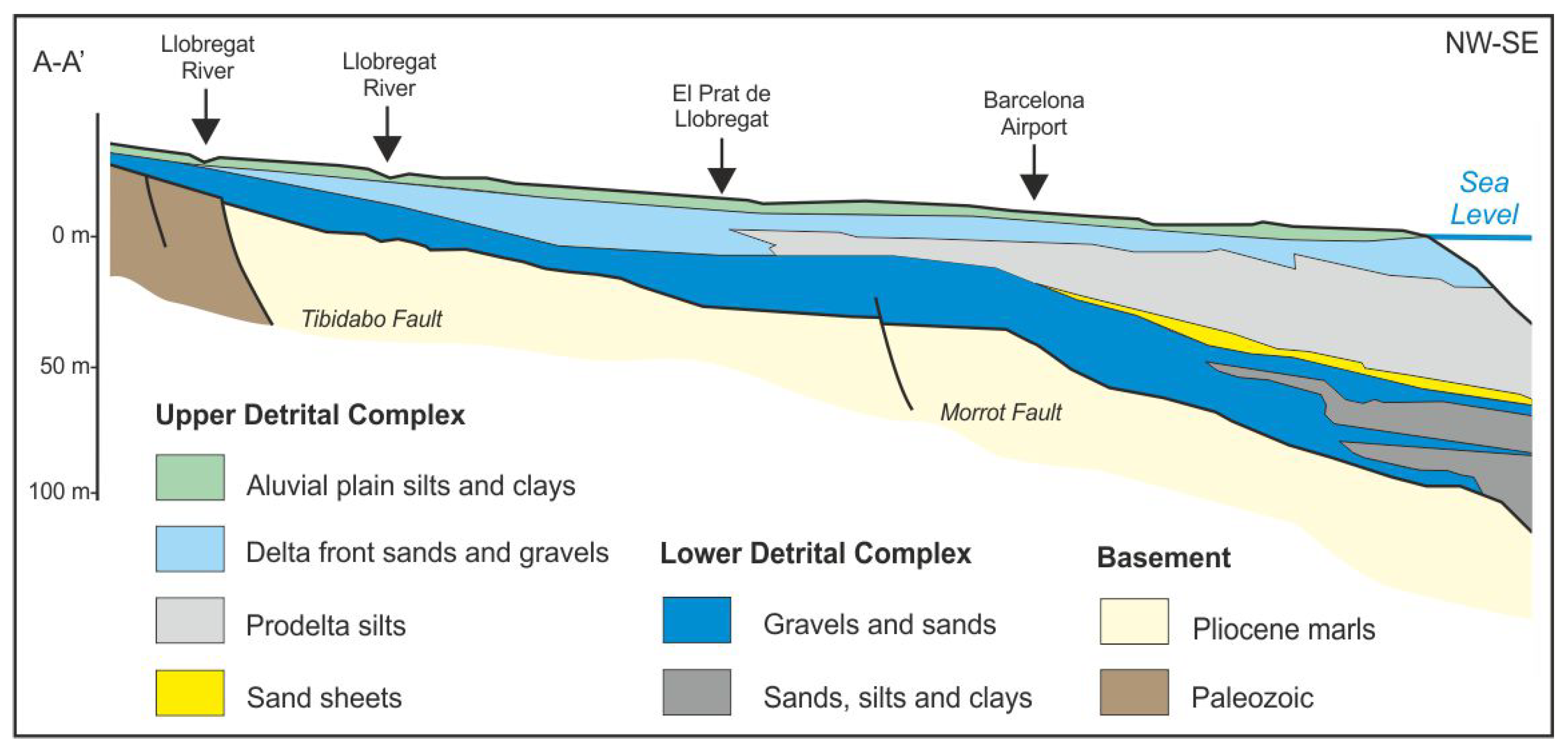
2. Study Area
3. Methodology
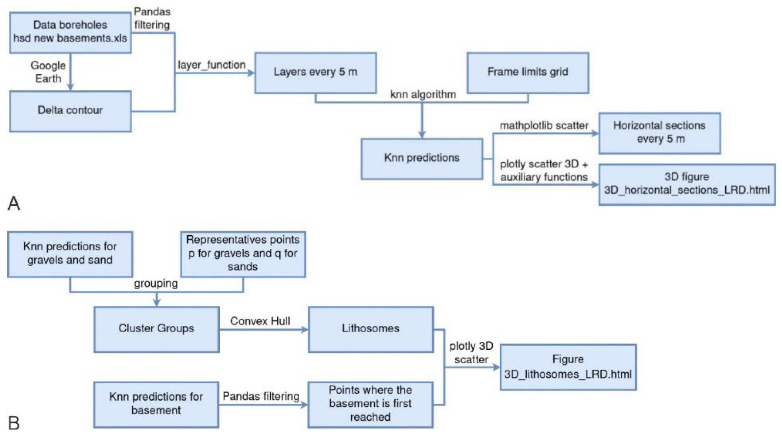
3.1. Data Compilation
3.2. Python Programing Language
3.3. KNN Algorithm
3.4. The 3D Mapping of the Granulometry Horizontal Sections
3.5. The 3D Mapping of the Stratigraphic Architecture and Basement Top Surface
4. Results
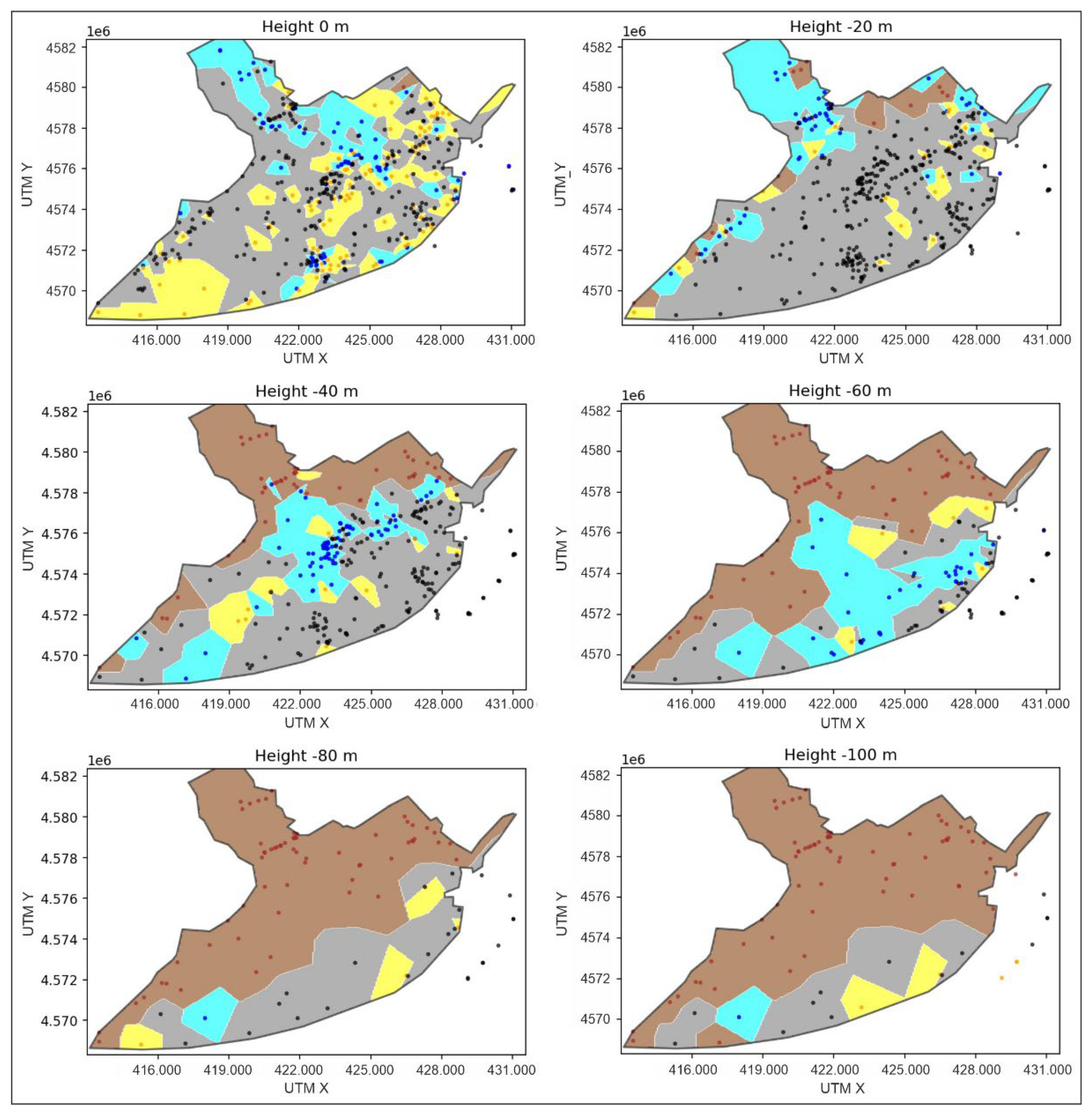
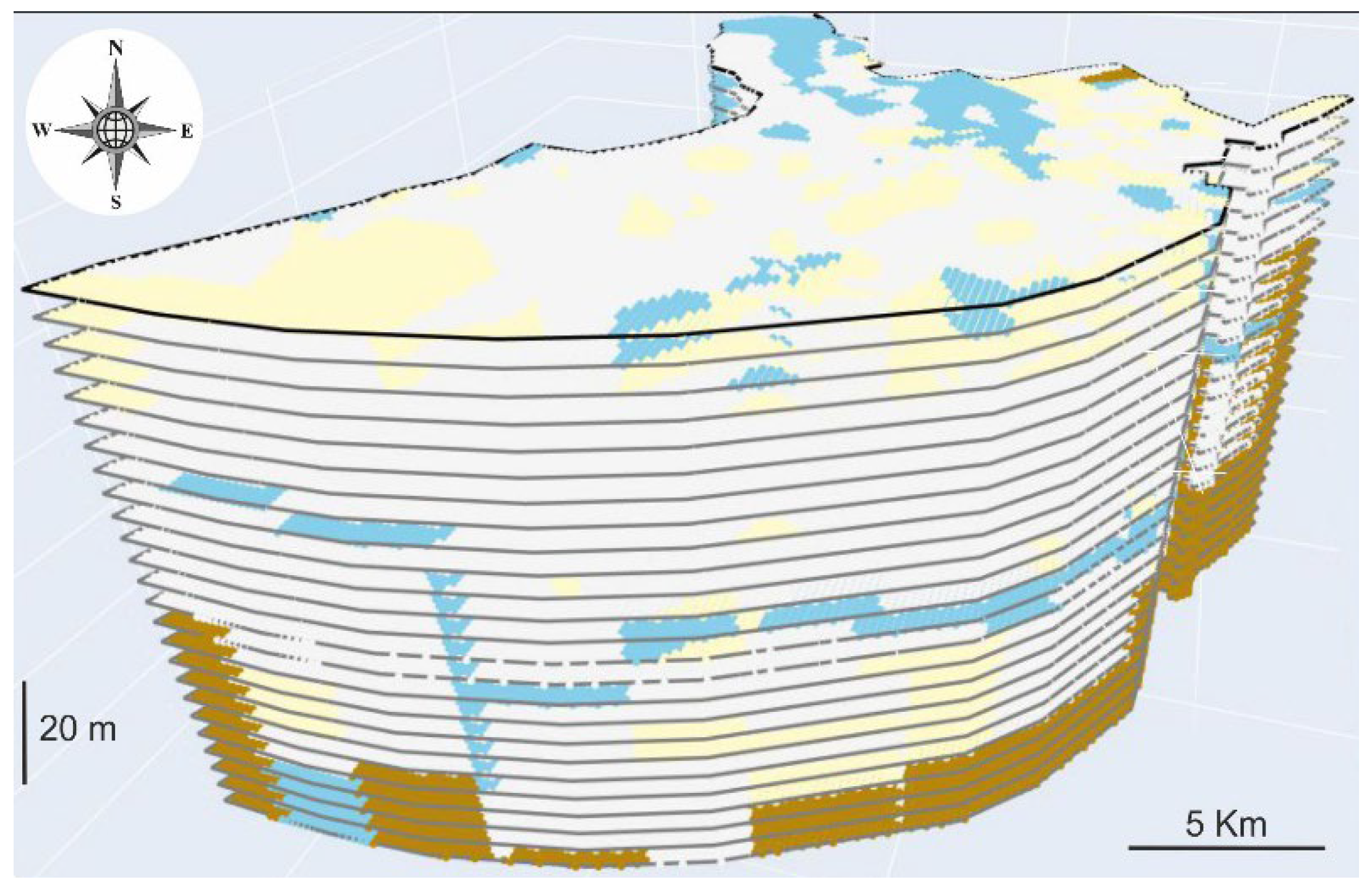
4.1. The 3D Mapping of the Granulometry Horizontal Sections
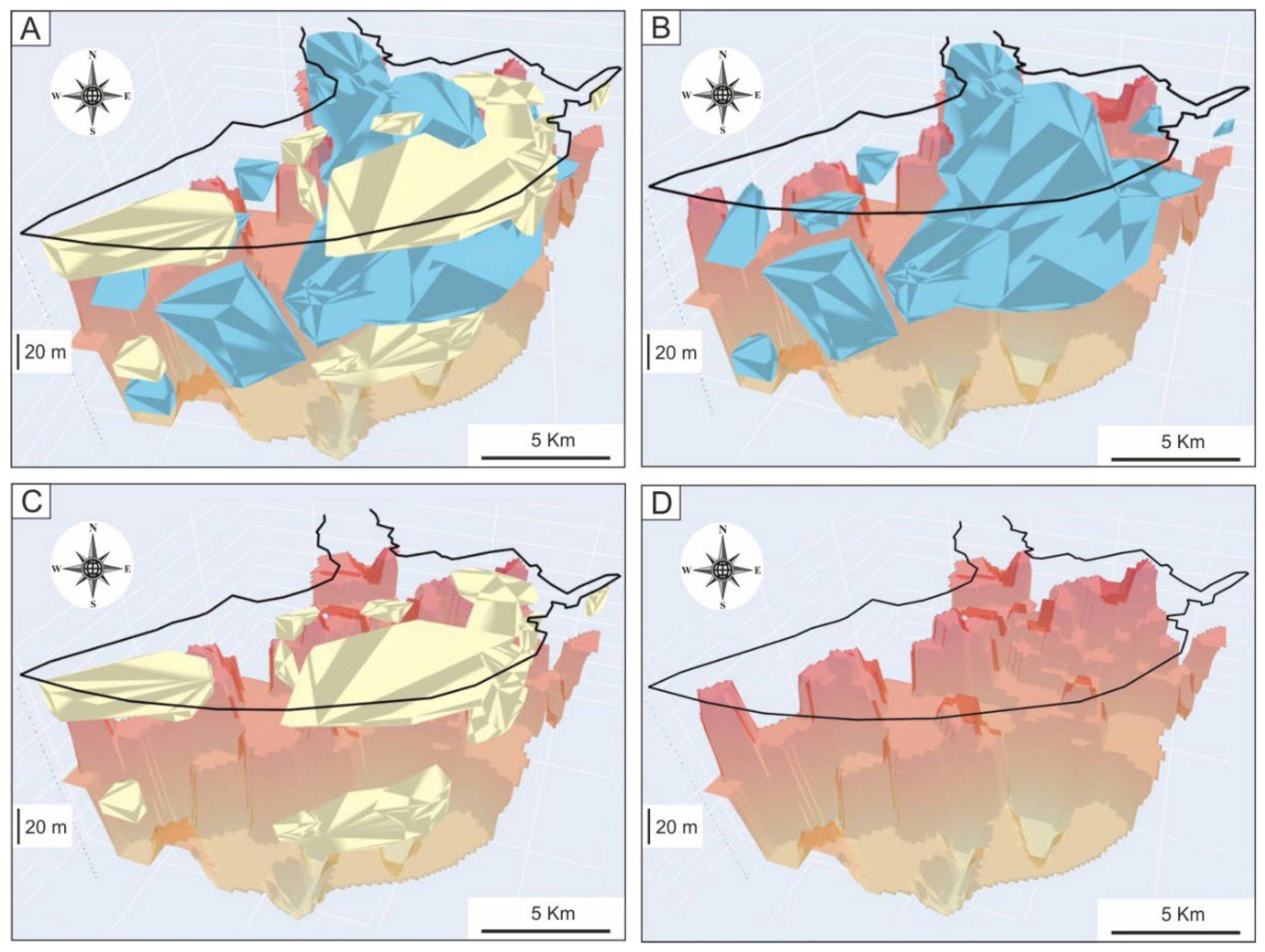
4.2. The 3D Mapping of the Stratigraphic Architecture and Basement Top Surface
5. Discussion and Conclusions
Supplementary Materials
Author Contributions
Funding
Institutional Review Board Statement
Informed Consent Statement
Data Availability Statement
Acknowledgments
Conflicts of Interest
References
- Jessell, M. Three-dimensional geological modelling of potential-field data. Comput. Geosci. 2001, 27, 455–465. [Google Scholar] [CrossRef]
- Wycisk, P.; Hubert, T.; Gossel, W.; Neumann, C. High-resolution 3D spatial modelling of complex geological structures for an environmental risk assessment of abundant mining and industrial megasites. Comput. Geosci. 2009, 35, 165–182. [Google Scholar] [CrossRef]
- Ford, J.; Mathers, S.; Royse, K.; Aldiss, D.; Morgan, D.J.R. Geological 3D modelling: Scientific discovery and enhanced understanding of the subsurface, with examples from the UK. Z. Dtsch. Ges. Geowiss. 2010, 161, 205–218. [Google Scholar] [CrossRef] [Green Version]
- Rohmer, O.; Bertrand, E.; Mercerat, E.D.; Régnier, J.; Pernoud, M.; Langlaude, P.; Alvarez, M. Combining borehole log-stratigraphies and ambient vibration data to build a 3D Model of the Lower Var Valley, Nice (France). Eng. Geol. 2020, 270, 105588. [Google Scholar] [CrossRef]
- GemPy: Open-Source 3D Geological Modeling. Available online: https://www.gempy.org (accessed on 9 June 2022).
- OSGeo: The Open Source Geospatial Foundation. Available online: https://www.osgeo.org/ (accessed on 9 June 2022).
- GeoPandas. Available online: https://geopandas.org/en/stable (accessed on 9 June 2022).
- Albion: 3D Geological Models in QGIS. Available online: https://gitlab.com/Oslandia/albion (accessed on 9 June 2022).
- GISgeography. 15 Python Libraries for GIS and Mapping. Available online: https://gisgeography.com/python-libraries-gis-mapping (accessed on 9 June 2022).
- Parpoil, B. Open Source and Geology. Available online: https://oslandia.com/en/2020/07/09/geologie-open-source (accessed on 9 June 2022).
- Hobona, G.; James, P.; Fairbairn, D. Web-based visualization of 3D geospatial data using Java3D. IEEE Comput. Graph. Appl. 2006, 26, 28–33. Available online: https://ieeexplore.ieee.org/document/1652923 (accessed on 12 July 2022). [CrossRef]
- Evangelidis, K.; Papadopoulos, T.; Papatheodorou, K.; Mastorokostas, P.; Hilas, C. 3D geospatial visualizations: Animation and motion effects on spatial objects. Comput. Geosci. 2018, 111, 200–212. [Google Scholar] [CrossRef]
- Semmo, A.; Trapp, M.; Jobst, M.; Doellner, J. Cartography-oriented design of 3D geospatial information visualization–overview and techniques. Cartogr. J. 2015, 52, 95–106. [Google Scholar] [CrossRef]
- Miao, R.; Song, J.; Zhu, Y. 3D Geographic Scenes Visualization Based on WebGL. In Proceedings of the 6th International Conference on Agro-Geoinformatics, Fairfax, VA, USA, 7–10 August 2017; IEEE: Fairfax, VA, USA, 2017; Volume 1, pp. 1–6. Available online: https://ieeexplore.ieee.org/stamp/stamp.jsp?tp=&arnumber=8046999 (accessed on 9 June 2022).
- Pyrcz, M. GeostatsGuy Lectures. Available online: https://www.youtube.com/c/GeostatsGuyLectures (accessed on 9 June 2022).
- Bullejos, M.; Cabezas, D.; Martín-Martín, M.; Alcalá, F.J. A Python Application for Visualizing the 3D Stratigraphic Architecture of the Onshore Llobregat River Delta in NE Spain. Water 2022, 14, 1882. Available online: https://www.mdpi.com/2073-4441/14/12/1882 (accessed on 12 July 2022). [CrossRef]
- Custodio, E. Seawater intrusion in the Llobregat Delta near Barcelona (Catalonia, Spain). In Groundwater Problems in the Coastal Areas, Studies and Reports in Hydrology; UNESCO: Paris, France, 1987; Volume 45, pp. 436–463. [Google Scholar]
- Medialdea, J.; Solé-Sabarís, L. Geological Map of Spain, Scale 1:50,000, Sheet n° 448. In El Prat de Llobregat, Memory and Maps; Geological Survey of Spain: Madrid, Spain, 1991; Available online: http://info.igme.es/cartografiadigital/geologica/Magna50Hoja.aspx?language=es&id=448 (accessed on 18 April 2022).
- Alonso, F.; Peón, A.; Rosell, J.; Arrufat, J.; Obrador, A. Geological Map of Spain, Scale 1:50,000, Sheet n° 421. In Barcelona, Memory and Maps; Geological Survey of Spain: Madrid, Spain, 1974; Available online: http://info.igme.es/cartografiadigital/geologica/Magna50Hoja.aspx?language=es&id=421 (accessed on 18 April 2022).
- Gámez, D.; Simó, J.A.; Lobo, F.J.; Barnolas, A.; Carrera, J.; Vázquez-Suñé, E. Onshore–offshore correlation of the Llobregat deltaic system, Spain: Development of deltaic geometries under different relative sea-level and growth fault influences. Sediment. Geol. 2009, 217, 65–84. [Google Scholar] [CrossRef]
- Almera, J. Mapa Geológico y Topográfico De La Provincia De Barcelona: Región Primera o De Contornos de la Capital Detallada, Scale 1:40,000, Memory and Maps, Diputación de Barcelona, Barcelona. 1891. Available online: https://cartotecadigital.icgc.cat/digital/collection/catalunya/id/2174 (accessed on 18 April 2022).
- Abarca, E.; Vázquez-Suñé, E.; Carrera, J.; Capino, B.; Gámez, D.; Batlle, F. Optimal design of measures to correct seawater intrusion. Water Resour. Res. 2006, 42, W09415. [Google Scholar] [CrossRef] [Green Version]
- Vázquez-Suñé, E.; Abarca, E.; Carrera, J.; Capino, B.; Gámez, D.; Pool, M.; Simó, T.; Batlle, F.; Niñerola, J.M.; Ibáñez, X. Groundwater modelling as a tool for the European Water Framework Directive (WFD) application: The Llobregat case. Phys. Chem. Earth 2006, 31, 1015–1029. [Google Scholar] [CrossRef]
- Postigo, C.; Ginebreda, A.; Barbieri, M.V.; Barceló, D.; Martín-Alonso, J.; de la Cal, A.; Boleda, M.R.; Otero, N.; Carrey, R.; Solà, V.; et al. Investigative monitoring of pesticide and nitrogen pollution sources in a complex multi-stressed catchment: The lower Llobregat River basin case study (Barcelona, Spain). Sci. Total Environ. 2021, 755, 142377. [Google Scholar] [CrossRef] [PubMed]
- Resolution 12956/1994. Cooperation Agreement on Infrastructure and Environment in the Llobregat Delta. In Official Journal of Spain; Ministry of Public Works, Transports and Environment: Madrid, Spain; Government of Spain: Madrid, Spain, 1994; Available online: https://www.boe.es/diario_boe/txt.php?id=BOE-A-1994-12956 (accessed on 18 April 2022).
- Official Statement. The Water Authority of Catalonia Creates the Technical Unit of the Llobregat Aquifers. In Official Journal of Catalonia; Department of the Environment and Housing, Government of Catalonia: Barcelona, Spain, 2004; Available online: https://govern.cat/salapremsa/notes-premsa/68710/agencia-catalana-aigua-crea-mesa-tecnica-dels-aqueifers-del-llobregat (accessed on 18 April 2022).
- Medialdea, J.; Solé-Sabarís, L. Geological Map of Spain, Scale 1:50,000, Sheet n° 420. In Hospitalet de Llobregat, Memory and Maps; Geological Survey of Spain: Madrid, Spain, 1973; Available online: http://info.igme.es/cartografiadigital/geologica/Magna50Hoja.aspx?language=es&id=420 (accessed on 18 April 2022).
- Llopis, N. Tectomorfología del Macizo del Tibidabo y valle inferior del Llobregat. Estud. Geogr. 1942, 3, 321–383. [Google Scholar]
- Solé-Sabarís, L. Ensayo de interpretación del Cuaternario Barcelonés. Misc. Barcinonensia 1963, 2, 7–54. [Google Scholar]
- Marqués, M.A. Les Formacions Quaternàries del Delta del Llobregat; Institut d’Estudis Catalans: Barcelona, Spain, 1984. [Google Scholar]
- Manzano, M. Estudio Sedimentológico del Prodelta Holoceno del Llobregat. Master’s Thesis, University of Barcelona, Barcelona, Spain, 1986. [Google Scholar]
- IGME. Geological Map of the Spanish Continental Shelf and Adjacent Areas, Scale 1:200,000, Sheet n° 42E. In Barcelona, Memory and Maps; Geological Survey of Spain: Madrid, Spain, 1989; Available online: https://info.igme.es/cartografiadigital/tematica/Fomar200Hoja.aspx?language=es&id=42E (accessed on 18 April 2022).
- IGME. Geological Map of the Spanish Continental Shelf and Adjacent Areas, Scale 1:200,000, Sheet n° 42. In Tarragona, Memory and Maps; Geological Survey of Spain: Madrid, Spain, 1986; Available online: https://info.igme.es/cartografiadigital/tematica/Fomar200Hoja.aspx?language=es&id=42 (accessed on 18 April 2022).
- Serra, J.; Verdaguer, A. La Plataforma Holocena en el Prodelta del Llobregat. In X Congreso Nacional de Sedimentología; Obrador, A., Ed.; University of Barcelona: Barcelona, Spain, 1983; Volume 2, pp. 49–51. [Google Scholar]
- Iribar, V.; Carrera, J.; Custodio, E.; Medina, A. Inverse modelling of seawater intrusion in the Llobregat delta deep aquifer. J. Hydrol. 1997, 198, 226–247. [Google Scholar] [CrossRef]
- Alcalá-García, F.J.; Miró, J.; García-Ruz, A. Sobre la intrusión marina en el sector oriental del acuífero profundo del delta del Llobregat (Barcelona, España). Breve descripción histórica y evolución actual. Bol. Real Soc. Española Hist. Nat. 2002, 97, 42–49. [Google Scholar]
- Alcalá-García, F.J.; Miró, J.; Rodríguez, P.; Rojas-Martín, I.; Martín-Martín, M. Actualización Geológica del Delta del Llobregat (Barcelona, España). Implicaciones Geológicas e Hidrogeológicas. In Tecnología de la Intrusión de Agua de Mar en Acuíferos Costeros: Países Mediterráneos; López-Geta, J.A., de la Orden, J.A., Gómez, J.D., Ramos, G., Mejías, M., Rodríguez, L., Eds.; Geological Survey of Spain: Madrid, Spain, 2003; Volume 1, pp. 45–52. [Google Scholar]
- Alcalá-García, F.J.; Miró, J.; Rodríguez, P.; Rojas-Martín, I.; Martín-Martín, M. Características estructurales y estratigráficas del substrato Plioceno del Delta de Llobregat (Barcelona, España)—Aplicación a los estudios hidrogeológicos. Rev. Geotemas 2003, 5, 23–26. [Google Scholar]
- Simó, J.A.; Gàmez, D.; Salvany, J.M.; Vàzquez-Suñé, E.; Carrera, J.; Barnolas, A.; Alcalá, F.J. Arquitectura de facies de los deltas cuaternarios del río Llobregat, Barcelona, España. Geogaceta 2005, 38, 171–174. [Google Scholar]
- Font, J.; Julia, A.; Rovira, J.; Salat, J.; Sanchez-Pardo, J. Circulación marina en la plataforma continental del Ebro determinada a partir de la distribución de masas de agua y los microcontaminantes orgánicos en el sedimento. Acta Geol. Hisp. 1987, 21, 483–489. [Google Scholar]
- Chiocci, F.L.; Ercilla, G.; Torres, J. Stratal architecture of Western Mediterranean Margins as the result of the stacking of Quaternary lowstand deposits below ‘glacio-eustatic fluctuation base-level’. Sediment. Geol. 1997, 112, 195–217. [Google Scholar] [CrossRef]
- Alcalá, F.J.; Martín-Martín, M.; García-Ruz, A. A lithology database from historical 457 boreholes in the Llobregat River Delta aquifers in northeastern Spain. Figshare Dataset 2020. [Google Scholar] [CrossRef]
- Python Programming Language. Available online: https://www.python.org (accessed on 9 June 2022).
- Numpy. Available online: https://numpy.org (accessed on 13 June 2022).
- Pandas. Available online: https://pandas.pydata.org/ (accessed on 13 June 2022).
- Plotly. Available online: https://plotly.com (accessed on 9 June 2022).
- Scipy. Available online: https://scipy.org (accessed on 13 June 2022).
- Scikit-learn. Available online: https://scikit-learn.org/stable/install.html#installation-instructions (accessed on 13 June 2022).
- GEODOSE. Available online: https://www.geodose.com/2019/09/3d-terrain-modelling-in-python.html (accessed on 13 June 2022).
- Gou, J.; Ma, H.; Ou, W.; Zeng, S.; Rao, Y.; Yang, H. A generalized mean distance-based k-nearest neighbor classifier. Expert Syst. Appl. 2019, 115, 356–372. [Google Scholar] [CrossRef]
- Pratama, H. Machine Learning: Using Optimized KNN (K-Nearest Neighbors) to Predict the Facies Classifications. In Proceedings of the 13th SEGJ International Symposium, Tokyo, Japan, 12–14 November 2018; Society of Exploration Geophysicists of Japan: Tokyo, Japan, 2018; Volume 1, pp. 538–541. [Google Scholar] [CrossRef]
- Wang, X.; Yang, S.; Zhao, Y.; Wang, Y. Lithology identification using an optimized KNN clustering method based on entropy-weighed co-sine distance in Mesozoic strata of Gaoqing field, Jiyang depression. J. Pet. Sci. Eng. 2018, 166, 157–174. [Google Scholar] [CrossRef]
- Huang, S.; Huang, M.; Lyu, Y. An Improved KNN-Based Slope Stability Prediction Model. Adv. Civ. Eng. 2020, 2020, 8894109. [Google Scholar] [CrossRef]
- Convex Hull Algorithm. Available online: https://docs.scipy.org/doc/scipy/reference/generated/scipy.spatial.ConvexHull.html (accessed on 9 June 2022).
- Parcerisa, D.; Gámez, D.; Gómez-Gras, D.; Usera, J.; Simó, J.A.; Carrera, J. Estratigrafía y petrología del subsuelo precuaternario del sector SW de la depresión de Barcelona (Cadenas Costeras Catalanas, NE de Iberia). Rev. Soc. Geol. España 2008, 21, 93–109. [Google Scholar]
- Salvany, J.M.; Aguirre, J. The Neogene and Quaternary deposits of the Barcelona city through the high-speed train line. Geol. Acta 2020, 18, 1–19. [Google Scholar] [CrossRef]
- Payton, R.L.; Chiarella, D.; Kingdon, A. The influence of grain shape and size on the relationship between porosity and permeability in sandstone: A digital approach. Sci. Rep. 2022, 12, 7531. [Google Scholar] [CrossRef]
- Boadu, F.K. Hydraulic conductivity of soils from grain-size distribution: New models. J. Geotech. Geoenviron. Eng. 2000, 126, 739–746. [Google Scholar] [CrossRef]
- Torskaya, T.; Shabro, V.; Torres-Verdín, C.; Salazar-Tio, R.; Revil, A. Grain shape effects on permeability, formation factor, and capillary pressure from pore-scale modeling. Transp. Porous Media 2014, 102, 71–90. [Google Scholar] [CrossRef]
- Nabawy, B.S. Estimating porosity and permeability using Digital Image Analysis (DIA) technique for highly porous sandstones. Arab. J. Geosci. 2014, 7, 889–898. [Google Scholar] [CrossRef]
- De Lima, O.A.; Sri, N. Estimation of hydraulic parameters of shaly sandstone aquifers from geoelectrical measurements. J. Hydrol. 2000, 235, 12–26. [Google Scholar] [CrossRef]
- Paz, C.; Alcalá, F.J.; Carvalho, J.M.; Ribeiro, L. Current uses of ground penetrating radar in groundwater-dependent ecosystems research. Sci. Total Environ. 2017, 595, 868–885. [Google Scholar] [CrossRef] [PubMed]
- Paz, C.; Alcalá, F.J.; Ribeiro, L. Ground penetrating radar attenuation expressions in shallow groundwater research. J. Environ. Eng. Geophys. 2020, 25, 153–160. [Google Scholar] [CrossRef]


Publisher’s Note: MDPI stays neutral with regard to jurisdictional claims in published maps and institutional affiliations. |
© 2022 by the authors. Licensee MDPI, Basel, Switzerland. This article is an open access article distributed under the terms and conditions of the Creative Commons Attribution (CC BY) license (https://creativecommons.org/licenses/by/4.0/).
Share and Cite
Bullejos, M.; Cabezas, D.; Martín-Martín, M.; Alcalá, F.J. A K-Nearest Neighbors Algorithm in Python for Visualizing the 3D Stratigraphic Architecture of the Llobregat River Delta in NE Spain. J. Mar. Sci. Eng. 2022, 10, 986. https://doi.org/10.3390/jmse10070986
Bullejos M, Cabezas D, Martín-Martín M, Alcalá FJ. A K-Nearest Neighbors Algorithm in Python for Visualizing the 3D Stratigraphic Architecture of the Llobregat River Delta in NE Spain. Journal of Marine Science and Engineering. 2022; 10(7):986. https://doi.org/10.3390/jmse10070986
Chicago/Turabian StyleBullejos, Manuel, David Cabezas, Manuel Martín-Martín, and Francisco Javier Alcalá. 2022. "A K-Nearest Neighbors Algorithm in Python for Visualizing the 3D Stratigraphic Architecture of the Llobregat River Delta in NE Spain" Journal of Marine Science and Engineering 10, no. 7: 986. https://doi.org/10.3390/jmse10070986