Article

Simulation Study on the Performance and Emission Parameters of a Marine Diesel Engine

1
College of Marine Engineering, Dalian Maritime University, Dalian 116206, China
2
Yangtze Delta Region Institute, Tsinghua University, Jiaxing 314006, China
*
Authors to whom correspondence should be addressed.
J. Mar. Sci. Eng. 2022, 10(7), 985; https://doi.org/10.3390/jmse10070985
Submission received: 27 June 2022 / Revised: 13 July 2022 / Accepted: 14 July 2022 / Published: 19 July 2022
(This article belongs to the Section Ocean Engineering)

Abstract

:
Development of intelligent ships requires marine diesel engine simulation models of high accuracy and fast response. In addition, with advent of tighter shipping air emissions regulations, such models are required to have emission prediction capabilities. In this article, such a model was developed and validated for a 30,000-ton bulk carrier main engine using MATLAB/Simulink. The simulation is based on mean value model, which predicts both the steady-state and dynamic performance of the engine. The results show that the steady-state performance parameters of the main engine are predicted within 2.2% error, and the exhaust emissions parameters are predicted within 7% error as compared to the bench test data from the engine manufacturer. The Maximum Continuous Rating (MCR) points at 100%, 75%, 50% and 25% of the E3 duty cycle were investigated with emphasis according to the diesel propulsion characteristics. In dynamic simulation, it is found that the compressor pressure fluctuation is greater than that of the exhaust pressure with the load variation. Furthermore, the compressor and the exhaust pipe have a similar temperature drop value (about 60 K) when the engine load changes from 100% to 50% MCR, and the exhaust pipe temperature fluctuation is more significant when the load varies from 50% to 25% MCR. The above results show the model’s good transient capability in simulating the dynamic characteristics of the engine. This model can be used especially for the development and control of marine diesel engines in intelligent ships as well as training-oriented marine engine and ship simulators.

1. Introduction

As the worldwide shipping activities are continuously growing, higher requirements are put forth towards the green shipping in order to limit the environmental impacts of maritime industry. The International Maritime Organization (IMO) has established a series of regulatory frameworks for the limitation of both the air pollutants, such as nitrogen oxides (NOx), and greenhouse gaseous emissions, primarily CO2 [1,2,3]. Especially, Annex IV of MARPOL Convention defines the Energy Efficiency Design Index (EEDI) for new ships, the Energy Efficiency for Existing Ship Index (EEXI), the Ship Energy Efficiency Management Plan (SEEMP), ship fuel oil Data Collection System (DCN) and the Carbon Intensity Indicator (CII) and CII Rating [4,5]. These regulations together focus on the reduction of both CO2 emissions and fuel consumption throughout the ship’s lifetime including ship design and ship operation.
On-board marine diesel engines are the main source of the above emissions and thus the reduction of shipping air emissions is highly influenced by design and operation of such engines. A good marine diesel engine needs to not only keep good steady-state and dynamic characteristics, but also improve fuel economy and minimize the emissions. To support this process, modeling techniques are used in order to realistically simulate the diesel engine. In order to meet these requirements, it is necessary for the marine diesel engine model to predict its performance and emissions at different loads and speeds. Moreover, the simulation of dynamic performance of diesel engine has a great significance for validating and optimizing the performance of diesel engine itself, for whole ship simulation and developing marine engine simulators for crew training.
For the above applications, the premise of ensuring the accuracy of the simulation results of the engine model together fast simulation speed should be selected. In 1989, E. Hendricks combined the advantages of the quasi-steady-state model and the volume method model to build a Mean Value Engine Model (MVEM) [6]. This work in this paper is based on the MVEM development principle and uses PID algorithm control to simulate the working process of the engine dynamically. It can observe the pressure and temperature vary with load in some key units, such as scavenge box, exhaust pipe and compressor.
In the MVEM, the diesel engine is normally divided into several relatively independent units, such as scavenging box, diesel cylinder, exhaust manifold, turbocharger, inter-cooler and governor. Various types of MVEM have been used in the past for the simulation of marine engines and the ship propulsion system under steady-state and transient conditions. A detailed description of the MVEM was given by Theotokatos [7]. The engine cylinder flow process was considered to take place continuously in this cycle mean value model, thus neglecting the intermittent nature of the engine cylinder processes. As a result, the engine cycle averaged temporal evolution of the engine operating parameters could be provided by this model, while the changes of in-cycle variation (e.g., per degree of crank angle) cannot be calculated. Wang [8] established a mean value model of the 6S60MC engine and added scavenging coefficients in the scavenging box modeling to make the prediction of the scavenging pressure variation with crank angle higher accuracy. Traditional MVEM could not simulate the working process of the cylinders dynamically, and the simulation and calculation of the volumetric model could be time consuming and error prone. Cao [9] established a new model that combined volumetric model and mean value model methods and used open-loop control to simulate the working process of the cylinder dynamically. This model could reflect not only some average parameters, but also pressure and temperature of cylinder in real time under different load.
In addition, in order to comply with the development of intelligent ships and emission management regulations, it is necessary to simulate the exhaust emission of diesel engines [10,11]. Charles [12] established a chemical kinetic model of high-temperature hydrocarbon oxidation in combustion, and the coefficients were validated by comparison with data from a wide range of experimental regimes. In Wetenberg’ study [13], the kinetics of NO formation and CO conversion in lean, premixed, hydrocarbon-air flames were discussed in terms of the elementary reactions involved. With the assumption of constant temperature and equilibrium O and OH concentrations, it was shown that simple, analytic solutions for NO and CO as a function of time would be derived. Through experimentation and Taguchi approach, Muqeem et al. [14] got the optimum combination of the input parameters of diesel engine including compression ratio, fuel injection timing, air temperature and air pressure to decrease hydrocarbon emission and smoke opacity under no load, half load and full load conditions. The above research works included multiple input parameters of diesel engine, a large number of experimental data and complex fuel oxidation reaction kinetics, so that these models could not rapidly reflect the variation of marine diesel engine exhaust emissions with load. They could not meet the requirements of future intelligent ship simulation model.
The MVEM techniques used in this research take a shorter execution time. The method is faster because it ignores detailed in-cylinder and crank angle-based calculations. Additionally, this modeling technique does not depend on the detail type of engine. In this article, the first-order differential equations were used for calculating some key working parameters of diesel engine, such as engine speed and scavenge box pressure, to reduce the simulation time. On the basis of analyzing the experimental data of engines, MVEM also used the empirical formula containing the indicated thermal efficiency to calculate the indicated torque and exhaust temperature, ignoring the complex working process in the cylinder. The engine exhaust gas carbon dioxide (CO2) emission was calculated using the approach of perfect combustion in excess air, whereas the nitrogen oxide (NOx) emission was estimated by calculating the nitric oxide (NO) instantaneous concentration. The way of calculating some incomplete combustion products such as carbon monoxide (CO) and hydrocarbon (HC) was based on the empirical formula method. The final amount of the incomplete combustion products can be calculated by subtracting the oxidized amount from the initially generated amount. The new approach for the engine propulsion characteristic modeling and exhaust emission description is adopted to instead of the traditional one (based on the actual cycle in-cylinders calculation model). It strongly reduced the engine transient computation time and made it possible to transform the simulation model into a real-time executable application. This simulation model can be used for the development and control of intelligent marine diesel engines, subsequently used as part of development of intelligent ships and also as part of training-oriented marine engine and ship simulators.

2. Model of Marine Diesel Engine

2.1. Overview of the Mean Value Engine Model (MVEM)

MVEM was established based on the laws of mass, energy conservation and ideal gas state equation. Combining with the character of quasi-static model and volumetric model, the engine was divided into several relatively independent volume units. Figure 1 shows the schematic diagram of a diesel engine. According to the characteristics of the thermal system of the marine turbocharged diesel engine in this article, the diesel engine was divided into several relatively independent instantaneous balance systems, and it was assumed that the gas composition, temperature and pressure at each point in each system were uniform.
Under steady-state operating conditions, the turbine is driven by exhaust gas and supplies energy to compressor pressurizing the air from atmosphere. The compressed air passes through the intercooler and enters the scavenging box for storage and supplying to engine cylinders. After entering the cylinders, the fresh air is mixed with the fuel and undergoes combustion reaction in the combustion chamber. The piston is pushed by high temperature and pressure mixture and drives the crankshaft, which means output work of the engine is transferred to propeller for ship propulsion. The exhaust gas is discharged into the atmospheric environment after the exhaust manifold and the exhaust turbine.
The block diagram of mean value model shown in Figure 1 was implemented in the MATLAB/Simulink as depicted in Figure 2. It included Proportion Integration Differentiation (PID) speed regulation module, compressor, scavenging box, cylinder, turbine and other subsystems. In order to avoid the emergence of algebraic ring, some memory modules were used to store the value in the current calculation step and calculate the next step.
For the simulation of the ship main engine, various input data are used. These include the engine geometric data, the compressor and turbine performance data, the engine ambient conditions and the empirical parameters for engine modelling. This model can observe (i.e., predict/estimate) many process parameters in the operation of diesel engine. In this paper, engine speed, scavenge pressure, scavenge temperature, exhaust pressure, exhaust temperature, compressor outlet temperature and mass flow of each part were selected as the observation objects. Using these parameters, the key performance parameters of diesel engine, such as output power and brake specific fuel consumption (BSFC), were calculated.

2.2. Engine Simulated

The 6RT-flex58T-D large two-stroke low-speed marine diesel engine produced by Wartsila company was chosen as the object for the simulation, which is the main engine of a 30,000-ton bulk carrier. The engine crankshaft is directly connected to the ship fixed pitch propeller via the ship shafting system. Information relating to engine geometry and other engine components is shown in Table 1, and fuel characteristics are shown in Table 2 and Table 3.

2.3. Mean Value Engine Model

2.3.1. Turbocharger

According to the pressure ratio π c and the speed of the turbocharger rotor n t c , the flow of the compressor q c and the isentropic efficiency of the compressor η c can be obtained from the characteristic map of the compressor [15,16,17]. Figure 3 is the compressor flow characteristic curve obtained by transforming two-dimensional map.
Then the compressor outlet temperature T c and the torque M c can be obtained through Equations (1) and (2):
T c = T b [ 1 + 1 η c ( π c k 1 k 1 ) ]    
M c = 30 π q c c p T b n t c η c ( π c k 1 k 1 )
where c p is the constant pressure specific heat capacity of air; k is the adiabatic coefficient of air, which is related to temperature; and T b is the outlet temperature of the filter, which can be directly used as the ambient temperature T a t m .
Similar to the compressor, the turbine also uses the static data look-up table to calculate the dynamic data. Different from the compressor, the turbine is generally simplified as a nozzle [18,19], and the engine exhaust mass flow q t is calculated by the following formula:
q t = μ t F T A φ 2 P e m ρ t          
where   μ t   is the flow coefficient, F T A   is the equivalent cross-sectional area of turbine nozzle,   φ   is a flow function including exhaust adiabatic index and expand rate and   ρ t   is the gas density in front of the turbine; P e m is the exhaust manifold pressure, which can be regarded as the inlet pressure of the turbine.
The torque generated by the turbine M t   and supplied to the compressor is calculated using the following formula:
M t = 30 π q t c p e T e m η t n t c [ 1 ( P t P e m ) k e 1 k e ]
where c p e is the constant pressure specific heat capacity of exhaust gas, T e m is the turbine inlet temperature, η t is the isentropic efficiency of the turbine, k e is the adiabatic coefficient of exhaust gas and P t is the backpressure of the turbine.
According to Newton’s second law of motion, the speed of turbocharger n t c can be obtained as follows:
d n t c d t = 30 π η m M t M c J t c
where η m is the mechanical efficiency of the rotor and J t c is the polar moment of inertia of the turbocharger rotor.

2.3.2. Intercooler

The air outlet temperature of the intercooler T i c is calculated by introducing a simplified method of cooling coefficient according to Formula (6):
T i c = T c η i c ( T c T c w )            
where η i c   is the cooling coefficient of the intercooler. The cooling efficiency of intercooler of marine large two-stroke diesel engine is very high [20], generally above 0.9. T c w is the cooling water temperature. The air pressure drop Δ P i n t across the intercooler can be calculated by the following formula:
Δ P i n t = 0.682 q c 2 44.53 q c + 88.61

2.3.3. Scavenging Box

In this model, the scavenging box is regarded as a container. According to the law of conservation of mass and energy and the ideal gas state equation, and ignoring the heat dissipation effect in the scavenging box, the change of pressure Δ P s c can be calculated by the following formula:
Δ P s c = k R V s c ( q c T i c q a T s c )
where V s c is the volume of scavenging box and q a is the compressed air flow into the cylinder, which can only represent the average mass flow. T s c is the temperature of compressed air in scavenging box and R   is the ideal gas constant.

2.3.4. Excess Air Coefficient

The excess air coefficient λ refers to the ratio of the actual amount of air supplied for combustion to the amount of air required q f for the complete combustion of theoretical fuel. The accuracy of the excess air coefficient has a vital impact on the accuracy of the MVEM. The calculation of excess air coefficient is shown in Formula (9):
λ = q a q f L 0      
where L 0 represents the theoretical air mass required for complete combustion of 1 kg fuel, which is 14.3 in this model. In this paper, the average mass flow of compressed air entering the cylinder can be calculated by the following formula [21,22]:
q a = N c y l η v n e 60 P s c V d R T s c
where N c y l is the number of cylinders, V d is the working volume of cylinder, n e is the speed of diesel engine and η v is the volumetric efficiency of the cylinder, which refers to the ratio of the actual intake volume of the cylinder to the cylinder volume during the intake stroke.

2.3.5. Indicated Torque and Exhaust Temperature

The indicated thermal efficiency η i of large low-speed diesel engine is a function of the excess air coefficient [23]. In order to avoid increasing model complexity, the model uses experimental data for calculation:
η i = 0.7844 λ 2 + 7.131 λ + 36.16 100
The indicated torque M i of diesel engine can be calculated according to the indicated thermal efficiency.
M i = 30 π η i q f H u n e
where H u is the calorific value of fuel. The exhaust temperature T e x of diesel engine is an important factor to determine the working state of turbocharger. The exhaust temperature can be calculated by the following formula:
T e x = T s c + ( 1 ε w η i ) H u ( 1 + λ L 0 ) c p e
where ε w is the cooling efficiency, which is corrected in this model. The cooling efficiency will decrease with the decrease of rotating speed.
Moreover, the modeling method of exhaust manifold is similar to that of scavenge box, the change of pressure Δ P e m across exhaust manifold can be calculated by the following formula:
Δ P e m = k e R V e m ( q t T e x q t T e m )
where V e m is total volume of exhaust manifold.

2.3.6. Friction Torque and Load Torque

According to the propeller characteristics, the load torque M L for this model is calculated using the following formula:
M L = K Q ρ n e 2 D 5
where D   is the diameter of the propeller and the propeller diameter used in this model is 6.7m, K Q is the torque coefficient and ρ is the seawater density. According to the average friction loss pressure P f and the working volume of the cylinder, the average friction loss power can be calculated, and then according to the relationship between torque, power and speed, the calculation formula of average friction torque M f is obtained as follows:
M f = 30 P f V d n e  
According to Newton’s second law of motion, the change in speed of diesel engine with time can be obtained:
d n e d t = 30 π M i M f M L J e + J s + J p
where J e , J s and J p are the moment of inertia of diesel engine, shafting and propeller, respectively.

2.3.7. Governor

For a large-scale two-stroke diesel engine, the speed regulating mechanism is generally modeled by PID algorithm [24]. The module control algorithm in this paper is shown below:
q f   = K p [ e ( t ) + 1 T i 0 t e ( t ) d t ]
The input of the module e ( t ) is the difference between the set speed and the actual speed. K p and T i are the proportional term coefficient and integral term coefficient of PID, respectively. In order to simplify the calculation, the calculation link of throttle control fuel supply is omitted, and the output result is the average mass flow of fuel q f . The power and BSFC of the engine are calculated through Formulas (19) and (20).
P = n e ( W i W f ) 9549
B S F C = q f ( t ) P
where P is the output power of the engine, W f is the average friction loss power and W i is the indicated power.

2.4. Pollutant Emission Calculation Model

2.4.1. Calculation Model of CO2

Assuming the molecular formula of the fuel is CaHbOcNdSe (where the coefficients c, d and e are generally close to 0). The actual number of air moles required can be calculated by introducing an excess air coefficient (the volume fraction of oxygen in the air under this condition is 21%).
n a i r = λ ( a + e + b 4 c 2 )   0.21  
The number of moles of exhaust gas n e x is calculated in Formula (22):
n e x = λ ( a + e + b 4 c 2 ) 0.21 + b 4 + d 2  
The average molar mass of exhaust gas M e x can be calculated by the following formula:
M e x = n a i r M a i r + 1 n e x
In addition to complete combustion of fuel, the proportion of substances produced by other products, such as CO, HC and NOx, in the volume of exhaust gas is less than 0.5% [25]. Therefore, when calculating the mass flow q C O 2 of complete combustion products such as CO2, it can be regarded as the complete combustion of fuel in excess air, which can be directly calculated by Equation (24):
q C O 2 = q t a n e x M C O 2 M e x
where M C O 2 is molar mass of CO2.

2.4.2. Calculation Model of NOX

The main component of NOx is NO, and the content reaches between 90% and 95%. Therefore, the NOx emission model of diesel engine mainly needs to calculate the generation of NO.
In this article, the simplified model proposed by previous research [26,27,28] is used to calculate the N O generation rate. In this model, only the instantaneous concentration is used for calculation, and the equilibrium concentration of N O and N is not assumed. Under this condition, the generation rate of N O is deduced as follows:
d ( N O ) d t = 2 k a 1 ( O ) ( N 2 ) k 1
k 1 = 1 ( N O ) 2 k 2 ( O 2 ) ( N 2 ) 1 + k b 1 ( N O ) k a 2 ( O 2 ) + k a 3 ( O H )
k 2 = k a 1 k a 2 k b 1 k b 2
where k a i and k b i   (i = 1,2,3) are the chemical reaction rate constants, which are related to the temperature in the cylinder. The concentration of oxygen and nitrogen is estimated by the concentration in the exhaust gas, and the concentration of O atom is calculated by Equation (28):
( O ) = 0.397 T 0.5 ( O 2 ) 0.5 e x p ( 31090 T )
The concentration of O H is calculated by using the formula:
( O H ) = 2.129 × 10 4 T 0.57 ( O 2 ) 0.5 ( H 2 O ) 0.5 e x p ( 4595 T )
The concentration of O 2 , H 2 O and N 2 is estimated by the concentration in the exhaust gas.

2.4.3. Calculation Model of CO

After combustion, the carbon in the fuel is discharged as the mixture of CO, HC and C O 2 . The way of calculating C O final generation is to subtract the amount of oxidized C O from the amount of initially generated C O . The calculation formulas of C O initial generation and oxidation are compiled based on the empirical formulas:
d m C O d t = d m C O i d t d m C O o x d t
where m C O is the final production mass of C O , m C O i is the initial production mass of C O and m C O o x is the oxidation mass of C O .
d m C O i d t = A C O i m f i P z B C O 1 e ( 12000 T z )
where m f i is the total mass of fuel injected into the cylinder.
d m C O o x d t = B C O 2 e ( T z 1102 )
where P z is the pressure in the cylinder, T z is the temperature in the cylinder and A C O i , B C O 1 , B C O 2 are the empirical coefficients, respectively, which depend on the diesel engine type and working condition. The calibration results of primary parameters are presented in Table 4.
There are some empirical formulars in the CO and HC emission model and calibration has to be carried out to correct these parameters in models. The result of calibration directly affects the accuracy of the model, and high predicting accuracy can be obtained within limited test data. In this paper, the ambient and gaseous emission data in the parent engine test report will be used for calibration. As the parent engine test method was selected as E3 cycle according to the propulsion characteristics, this 100% MCR point is calibrated first and used as the reference point for the other load. The diesel model has been calibrated in various load according to the test report of the parent diesel engine.

2.4.4. Calculation Model of HC

In this paper, the method of calculating the final generation of H C is similar to the method of calculating C O . In this calculation model, the total amount of fuel injected into the combustion chamber and evaporated is taken as the initial total amount of H C . The final generation of H C is calculated by subtracting the amount of oxidized H C during combustion [12,29,30].
d m H C o x d t = A H C o x m O 2 P z B H C o x T z 5 e ( E H C o x R z T z )            
where m H C o x is the oxidation mass of H C and m O 2 is the mass of oxygen.
m H C = m f 0 t d m H C o x d t  
where m H C is the final production mass of H C and m f is the total mass of fuel volatized in the combustion chamber, meaning the initial total amount of H C ; R z is the gas constant in the cylinder and E H C o x is 1.5576 × 10⁵ kJ/kmol. A H C o x and B H C o x are the empirical coefficients, which depend on the diesel engine type and working condition. The calibration results of primary parameters are presented in Table 4.

3. Result and Discussion

3.1. Propulsion Performance Simulation

3.1.1. Steady-State Simulation

For the sake of completeness, the modeling approach was validated by comparing simulation results and experimental data from the parent engine test report including power, BSCF and exhaust gas temperature. The technical sheet carried out 12 working condition points test of diesel engine propulsion characteristics at 110%, 100%, 95%, 90%, 85%, 80%, 75%, 70%, 60%, 50%, 40% and 25% of MCR in turn.
In the speed setting module, the speed is set according to 110%, 100%, 95%, 90%, 85%, 80%, 75%, 70%, 60%, 50%, 40% and 25% of MCR, respectively. The results and relative errors are shown in Figure 4a–c. It can be seen that relative error of the output power remains between −1.13 and 0.21%, and the relative error of Break-Specific Fuel Consumption (BSFC) is between −1.35 and 1.97%, which verifies the correctness of the model. Due to some corrections in the modeling of cooling efficiency, the relative error of exhaust temperature is between −2.2 and 0.2%, which can meet the requirements of the simulation accuracy.

3.1.2. Dynamic Simulation

This dynamic simulation is mainly to observe the transient response ability of the model under the condition of sudden increase and decrease of the set speed. The dynamic simulation model in this paper chose four working points shown in Table 5 to examine the model ability to capture the engine transient response at different load conditions.
In the case (1), changes in the engine speed setpoint from 105 rpm to 95.4 rpm and from 95.4 rpm to 105 rpm are applied at the 10th and 70th second of the run, respectively. The results of dynamic simulation runs are given in Figure 5a,b. In the case (2), the simulation runs are applying to engine load changing from 75% to 50% MCR at the 10th second and from 50% to 75% MCR at the 70th second. Meanwhile, the engine speed changes from 95.4 rpm to 83.3 rpm during the unloading period and then from 83.3 rpm to 95.4 rpm during the loading period. The results of dynamic simulation are given in Figure 5c,d. For further investigating the engine model prediction capability at the low load, the engine operation from 50% to 25% MCR is simulated, and the results are presented in Figure 5e,f in the case (3).
For the case (1), the point A corresponds to the simulation starting point (100% load), and the engine load changes to the point B at the 10th second. The compressor pressure drops from 4.56 bar to 2.92 bar and the exhaust pressure drops from 4.25 bar to 2.72 bar, which means more pressure drop happens in the compressor. In addition, a similar temperature decreasing amount happens in the compressor and the exhaust pipe, which is about 60 K. The case (2) simulates the engine transient operation with load changes 75–50–75%. The compressor pressure drops from 2.92 bar to 1.86 bar from the point B to the point C, and the exhaust pressure drops to the same pressure value with the compressor at the point C. The compressor has a more pressure drop amount than the exhaust pipe about 0.21 bar in the unloading period. Meanwhile, the compressor temperature drops from 425K to 365 K and the exhaust temperature drops from 645 K to 598 K, the temperature drop amount of the compressor is more than the exhaust pipe about 13 K. For further investigating the engine model prediction capability at low loads, a transient engine operation from 50% load to 25% load is simulated in the case (3). The result shows that the compressor pressure drops from 1.86 bar to 1.26 bar and the exhaust pressure drops from 1.87 bar to 1.43 bar. The exhaust pipe has a higher pressure value than the compressor at the point D about 0.16 bar. The compressor temperature drops from 365 K to 321 K and the exhaust temperature drops from 598 K to 460 K, the temperature drop amount of the exhaust pipe is more than the compressor about 94K from the point C to the point D.
In summary, the cylinder pressure difference is calculated to be positive (compressor pressure is greater than the exhaust pressure) when the diesel engine load is more than 50%. When the diesel engine load is below 50% of MCR, the cylinder pressure difference is calculated to be negative (compressor pressure is lower than the exhaust pressure). This illustrates that the compressor pressure fluctuation is greater than that of the exhaust pressure with the load variation. Moreover, the compressor and the exhaust pipe have a similar temperature drop value when the engine load changes from 100% to 50% MCR, but the exhaust pipe temperature fluctuation is more significant when the load varies from 50% to 25% MCR.

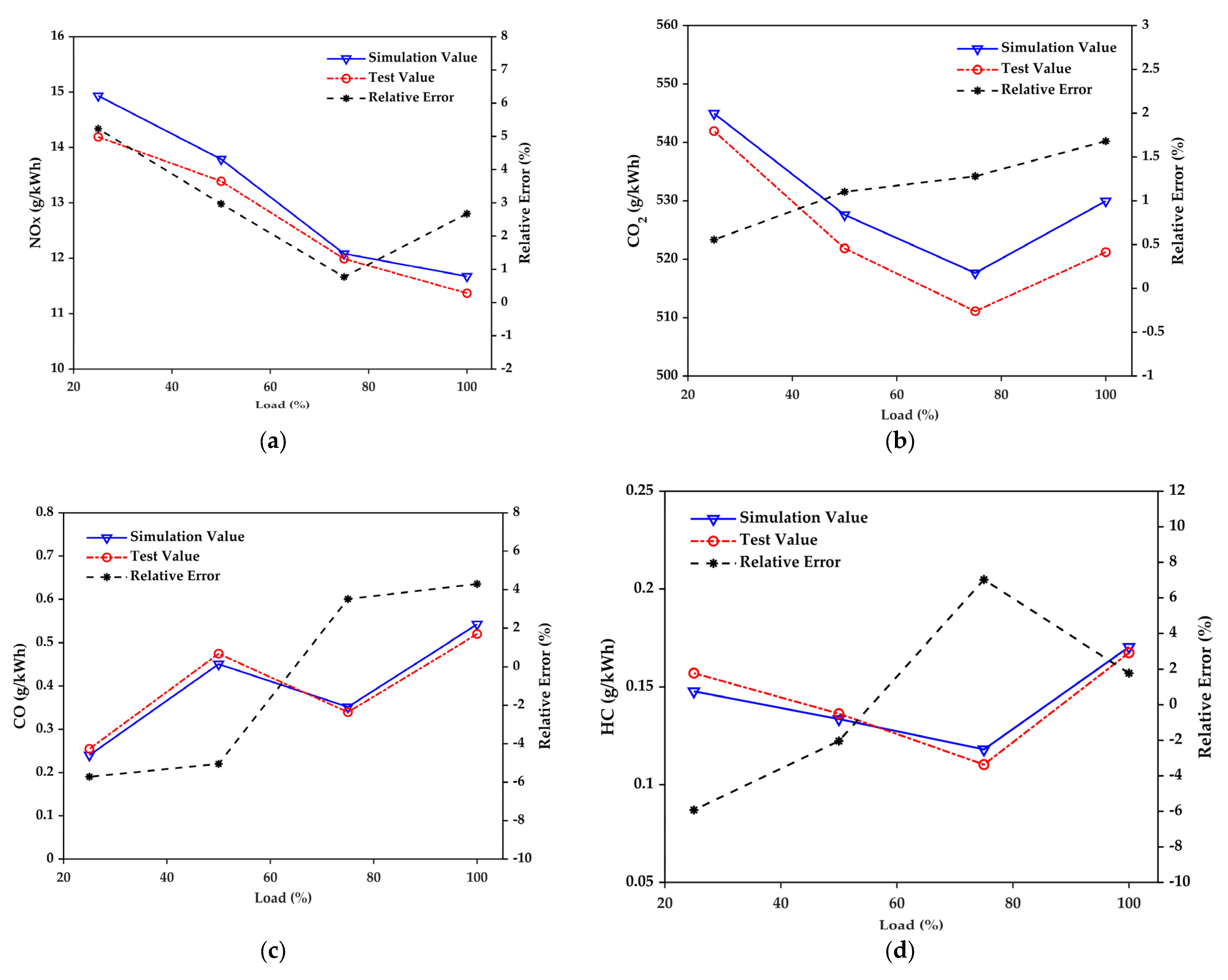
3.2. Emission Simulation

Marine engine emission gas analysis system was supplied by Dalian Guangming Special Gas Ch Research Institute using the HORIBA AIA-240, FAC-246 and IMA-241 Analyzer. This system could analysis the compositions of diesel engine exhaust gas including NOx, O2, CO2, CO and HC. The system inserted the sampling pipe into the exhaust pipe, which is 12 m away from the outlet of diesel engine cylinders and measured the exhaust gas with error below 0.79% according to the parent engine test report. The parent engine test method was selected as E3 duty cycle according to the propulsion characteristics, so that the technical sheet carried out four working condition points (100%, 75%, 50%, 25% of MCR) exhaust emission test results, which is the same as shown in Table 5. The simulation result of excess air coefficient is shown in Figure 6, which has a significant effect on diesel engine emissions.
For the marine main engine in this article, the NOx specific mass flow shows a decreasing trend with the increase of load in Figure 7a. At these four loads, the calculated and measured values show the same change trend, and the relative errors at 25%, 50%, 75% and 100% load are 5.23%, 2.97%, 0.77% and 2.67%, respectively.
According to Figure 7b, the difference between the simulated specific mass flow of CO2 and the test mass flow is very slight and maintain good consistency with the trend of BSFC in Figure 4b, which proves the reliability of complete combustion product emission model. The relative errors at 25%, 50%, 75% and 100% load are 0.56%, 1.10%,1.28% and 1.68%, respectively. The specific emission of CO2 decreases firstly and then increases with the increase of load. This is mainly due to excess air coefficient decreasing firstly and then increasing with the increase of load, which is the key parameter affecting the emission of CO2.
After being injected into the combustion chamber at high pressure, the fuel directly forms a combustible mixture with excess air in the cylinder and burns quickly. Due to the excess air coefficient being between 1.5 and 3 under most operating conditions of the diesel engine, the emissions of CO and HC from the marine engine are slight.
The emission of CO is largely determined by the excess air coefficient. In Figure 7c, the trend of CO is opposite to that of excess air coefficient when the load is below 75% of MCR. The fuel and air of diesel engine are mixed unevenly, so that there are always areas with less air and low temperature in the combustion chamber. Moreover, the residence time of reactants in the combustion area is short, which is not enough to complete the combustion process and generate CO emission. At high loads (>75% MCR), the maximum reaction temperature in the cylinder reaches more than 1600 K and the excess air coefficient is less than 3, as shown in Figure 6. As combustion products, CO2 and H2O will undergo pyrolysis reaction to produce CO under high cylinder temperature. Furthermore, a large amount of soot is generated in the oil-rich and lean oxygen area of mixture combustion, and the soot is oxidized to generate CO with excess oxygen. As a result, the specific mass flow of CO is increasing with a high load of the diesel engine. As the simulation result, the relative errors of CO emission model at 25%, 50%, 75% and 100% load are −5.72%, −5.05%, 3.51% and 4.30%, respectively.
As shown in Figure 7d, the simulation errors of HC emission at 25%, 50%, 75% and 100% load are −5.92%, −2.04%, 7% and 1.77%, respectively, and the specific flow of HC decreases with the load increasing from 25% to 75% of MCR. Due to the low temperature of the mixture gases near the cylinder wall, there is a thin boundary layer (quenching layer) nearby the cylinder wall maintaining a temperature below the spontaneous combustion temperature of the mixture, and the flames will be extinguished being close to the cylinder wall. The mixture gases containing HC in the quenching layer directly enters the exhaust without complete combustion. Especially at low load, the temperature of the combustion chamber wall is particularly low, causing the quenching layer to be thick and the mixture gas to have a low temperature. As a result of that, more HC will be generated at a low load.
In addition, there are various narrow gaps in the diesel engine combustion chamber, such as the gap between the piston bank and the cylinder wall, the sealing belt slit formed by the exhaust valve and the valve seat surface, etc. The flames cannot enter these gaps, which are small to a certain extent, so that some amount of HC in the gaps cannot be oxidized. During the compression and combustion stroke, more mixture gases will be squeezed into these gaps due to the pressure rising in the cylinders. After the piston passing the Top Dead Center (TDC), the mixture gases in gaps will return to the cylinders. Nevertheless, the oxygen concentration and temperature in the cylinder is decreased, so that the reoxidation proportion of the mixture flowing back to the cylinder is small.
At high load (>75% load), a large amount of soot will be produced from the oil-rich and lean oxygen area of mixture combustion. However, there are areas with the temperature lower than the soot generation temperature in the over concentrated mixture, which will generate liquid HC and be further volatilized out of the cylinder. Therefore, the specific flow of HC will increase rapidly at high load.

4. Conclusions

In this article, a mean value engine model (MVEM) of a ship’s main diesel engine was developed in MATLAB/Simulink with high accuracy and fast dynamic performance, which is especially helpful when used for more advanced intelligent ships. The model consists of two main parts: the engine power performance and the emissions. The model was then validated with experimental data. When applied to a two-stroke low-speed marine diesel engine of a 30,000-ton bulk carrier, the main conclusions are as follows:
  • When compared against the engine’s actual performance data, the relative error of major parameters from this model in steady-state simulation is within 2.2%, indicating a decent high accuracy.
  • The exhaust emissions models of CO2, CO, HC and NOX are established as a function of the load, and the relative error is found to be within 7%.
  • Three particular dynamic processes with sudden increase and decrease of the engine load at corresponding engine’s speed are simulated. The pressure of the compressor varies more greatly than that at the exhaust pipe under load variations and the exhaust pipe temperature fluctuation is more significant when the load varies from 50% to 25% MCR.
Due to the satisfying prediction capability as well as fast performance, the marine diesel engine model presented in this article can be used for a number of purposes including (1) as part of ship simulators for training purposes and (2) as part of an entire ship model voyage and operation simulation. In addition, the transient characteristics of the main engine can be obtained from this model, which can be used to study the interaction between hull, engine and propeller or to design the control strategy of marine diesel engines.

Author Contributions

Conceptualization, R.X. and Y.J.; methodology, R.X. and C.L.; software, R.X. and C.L.; validation, R.X. and C.L.; formal analysis, R.X.; investigation, R.X. and Z.W.; resources, R.X. and J.Z. (Jinguo Zhai); data curation, J.Z. (Jinguo Zhai) and C.L.; writing—original draft preparation, R.X.; writing—review and editing, Z.W., J.Z. (Jifeng Zhang), Y.J. and Z.B.; visualization, Z.W. and Z.B.; supervision, Y.J.; project administration, Z.W.; funding acquisition, Y.J. All authors have read and agreed to the published version of the manuscript.

Funding

This research was funded by National Key Research and Development Program of China (Grant No.: SQ2019YFE011597), China Postdoctoral Science Foundation (Grant No.: 2021M690496, 2020M670724), National Natural Science Foundation of China (Grant No.: 51876019, 52106225), the Dalian Outstanding Scientific and Technological Talents Program (Grant No.: 2020RJ03), and the Fundamental Research Funds for the Central Universities of China (Grant No.: 3132019331).

Institutional Review Board Statement

Not applicable.

Informed Consent Statement

Not applicable.

Data Availability Statement

Not applicable.

Acknowledgments

The authors thank Dalian Maritime University and Yangtze Delta Region Institute of Tsinghua University for their support.

Conflicts of Interest

The authors declare no conflict of interest. The founding sponsors had no role in the design of the study; in the collection, analyses, or interpretation of data; in the writing of the manuscript, and in the decision to publish the results.

References

  1. Yuan, Y.; Wang, J.; Yan, X.; Shen, B.; Long, T. A review of multi-energy hybrid power system for ships. Renew. Sust. Energ. Rev. 2020, 132, 110081. [Google Scholar] [CrossRef]
  2. Inal, O.B.; Charpentier, J.; Deniz, C. Hybrid power and propulsion systems for ships: Current status and future challenges. Renew. Sust. Energ. Rev. 2022, 156, 111965. [Google Scholar] [CrossRef]
  3. Third IMO Greenhouse Gas Study 2014. Available online: https://www.imo.org/en/OurWork/Environment/Pages/Greenhouse-Gas-Studies-2014.aspx (accessed on 1 July 2014).
  4. IMO MEPC.328 Full MARPOL Annex VI. Available online: https://imorules.com/MEPCRES_328.75.html (accessed on 17 June 2021).
  5. Resolution MEPC.304 Initial IMO Strategy on Reduction of GHG Emissions from Ships. Available online: https://wwwcdn.imo.org/localresources/en/KnowledgeCentre/IndexofIMOResolutions/MEPCDocuments/MEPC.304(72).pdf (accessed on 13 April 2018).
  6. Hendricks, E. Mean Value Modeling of Large Turbo-charged Two-Stroke Diesel Engines. SAE 1989, 890564. Available online: https://www.sae.org/publications/technical-papers/content/890564/ (accessed on 13 July 2022).
  7. Theotokatos, G. On the cycle mean value modelling of a large two-stroke marine diesel engine. Proc. Inst. Mech. Eng. Part M J. Eng. Marit. Environ. 2010, 224, 193–205. [Google Scholar] [CrossRef]
  8. Haiyan, W.; Ren, G.; Zhang, J. Dynamic Modeling of Large Two-Stroke Marine Diesel Engine. Trans. CSICE 2006, 24, 452–458. [Google Scholar]
  9. Hui, C.; Peili, W.; Jundong, Z. Modeling and Simulation of Working Process of Marine Diesel Engine with a Comprehensive Method. Int. J. Comput. Inform. Syst. and Ind. Manage. Appl. 2013, 5, 480–487. [Google Scholar]
  10. Han, Z.; Zou, T.; Wang, J.; Dong, J.; Deng, Y.; Pan, X. A Novel Method for Simultaneous Removal of NO and SO2 from Marine Exhaust Gas via In-Site Combination of Ozone Oxidation and Wet Scrubbing Absorption. J. Mar. Sci. Eng. 2020, 8, 943. [Google Scholar] [CrossRef]
  11. Yusuf, A.A.; Inambao, F.L.; Ampah, J.D. Evaluation of biodiesel on speciated PM2.5, organic compound, ultrafine particle and gaseous emissions from a low-speed EPA Tier II marine diesel engine coupled with DPF, DEP and SCR filter at various loads. Energy 2022, 239, 121837. [Google Scholar] [CrossRef]
  12. Charles, K.W.; Frederick, L.D. Chemical kinetic modeling of hydrocarbon combustion. Prog. Energy Combust. Sci. 1984, 10, 1–57. [Google Scholar]
  13. Westenberg, A.A. Kinetics of NO and CO in Lean, Premixed Hydrocarbon-Air Flames. Combust. Sci. Technol. 1971, 4, 59–64. [Google Scholar] [CrossRef]
  14. Muqeem, M.; Sherwani, A.F.; Ahmad, M.; Khan, Z.A. Optimization of diesel engine input parameters for reducing hydrocarbon emission and smoke opacity using Taguchi method and analysis of variance. Energ. Environ. 2018, 29, 410–431. [Google Scholar] [CrossRef]
  15. Altosole, M.; Campora, U.; Figari, M.; Laviola, M.; Martelli, M. A Diesel Engine Modelling Approach for Ship Propulsion Real-Time Simulators. J. Mar. Sci. Eng. 2019, 7, 138. [Google Scholar] [CrossRef] [Green Version]
  16. Taburri, M.; Chiara, F.; Canova, M.; Wang, Y. A model-based methodology to predict the compressor behavior for the simulation of turbocharged engines. Proc. Inst. Mech. Eng. Part D J. Auto. Eng. 2012, 226, 560–574. [Google Scholar] [CrossRef]
  17. Guan, C.; Theotokatos, G.; Zhou, P.; Chen, H. Computational investigation of a large containership propulsion engine operation at slow steaming conditions. Appl. Energy 2014, 130, 370–383. [Google Scholar] [CrossRef] [Green Version]
  18. Hountalas, D.T.; Kouremenos, D.A.; Sideris, M. A Diagnostic Method for Heavy-Duty Diesel Engines Used in Stationary Applications. Trans. ASME 2004, 126, 886–898. [Google Scholar] [CrossRef]
  19. Ernst, E.S.; Gary, L.B. Mathematical Simulation of a Large Turbocharged Two-Stroke Diesel Engine. SAE 1971, 710176, 733–768. [Google Scholar]
  20. Zhu, J. Modeling and Simulating of Container Ship’s Main Diesel Engine. Proc. IMECS 2008, 2, 19–21. [Google Scholar]
  21. Piero, A.; Giorgio, M.; Davide, M. Air-Fuel Ratio Control for a High Performance Engine using Throttle Angle Information. SAE 1999, 1999-01-1169. Available online: https://www.sae.org/publications/technical-papers/content/1999-01-1169/?PC=DL2BUY (accessed on 13 July 2022).
  22. John, R.; Wagner, D.M.; Dawson, L. Nonlinear Air-to-Fuel Ratio and Engine Speed Control for Hybrid Vehicles. IEEE Trans. Veh. Technol. 2003, 52, 184–195. [Google Scholar]
  23. Jensen, J.P.; Kristensen, A.F.; Sorenson, S.C.; Houbak, N.; Hendricks, E. Mean Value Modeling of a Small Turbocharged Diesel Engine. SAE 1991, 910070. Available online: https://saemobilus.sae.org/content/910070 (accessed on 13 July 2022).
  24. Damir, R.; Asgeir, J.S.; Tor, A.J. Inertial Control of Marine Engines and Propellers. IFAC Proc. Vol. 2007, 40, 323–328. [Google Scholar]
  25. Theotokatos, G.; Tzelepis, V.A. computational study on the performance and emission parameters mapping of a ship propulsion system. Proc. Inst. Mech. Eng. Part M J. Eng. Marit. Environ. 2015, 229, 58–76. [Google Scholar] [CrossRef] [Green Version]
  26. Roberto, F.; Ezio, S. A real time zero-dimensional diagnostic model for the calculation of in-cylinder temperatures, HRR and nitrogen oxides in diesel engines. Energ. Convers. Manag. 2014, 79, 498–510. [Google Scholar]
  27. Psota, M.A.; Mellor, A.M. Dynamic Application of a Skeletal Mechanism for DI Diesel NOx Emissions. SAE 2001, 2001-01-1984. [Google Scholar]
  28. Mellor, A.M.; Mello, J.P.; Duffy, K.P.; Easley, W.L.; Faulkner, J.C. Skeletal Mechanism for NOx Chemistry in Diesel Engines. SAE 1998, 981450. Available online: https://www.jstor.org/stable/44746494 (accessed on 13 July 2022).
  29. Meng, Z.; Yang, D.; Yan, Y. Study of carbon black oxidation behavior under different heating rates. J. Therm. Anal. Calorim. 2014, 118, 551–559. [Google Scholar] [CrossRef]
  30. Hiroyasu, H.; Kadota, T. Models for Combustion and Formation of Nitric Oxide and Soot in Direct Injection Diesel Engines. SAE 1976, 760129, 513–526. [Google Scholar]
Figure 1. Schematic diagram of modeled diesel engine.
Jmse 10 00985 g001
Figure 2. Simulation diagram of diesel engine in Simulink.
Jmse 10 00985 g002
Figure 3. Character flow curve of compressor.
Jmse 10 00985 g003
Figure 4. Comparison of simulation results to experimental data in steady-state performance: (a) power variation trend with load, (b) BSFC variation trend with load and (c) exhaust temperature variation trend with load.
Jmse 10 00985 g004
Figure 5. Transient response of the engine performance parameters with the change of setting speed: (a) pressure curves of the compressor and the exhaust pipe in case (1), (b) temperature curves of the compressor and the exhaust pipe in case (1), (c) pressure curves of the compressor and the exhaust pipe in case (2), (d) temperature curves of the compressor and the exhaust pipe in case (2), (e) pressure curves of the compressor and the exhaust pipe in case (3) and (f) temperature curves of the compressor and the exhaust pipe in case (3).
Jmse 10 00985 g005aJmse 10 00985 g005b
Figure 6. Excess air coefficient variation trend with load.
Jmse 10 00985 g006
Figure 7. Comparison of simulation results to experimental data in steady-state performance: (a) emissions of NOX variation trend with load, (b) emissions of CO2 variation trend with load, (c) emissions of CO variation trend with load and (d) emissions of HC variation trend with load.
Jmse 10 00985 g007
Table 1. Technical parameters of the parent engine.
NameParameter
Engine type6RT-flex58T-D
Number of cylinders6
MCR power [kW]10,850
MCR BSFC [g/kWh]162
MCR speed [r/min]105
Bore [mm]580
Stroke [mm]2416
Compression ratio15
Maximum cylinder pressure [bar]155.2
Mean effective pressure [bar]16.2
Turbocharger2 × A165-L34
Air cooler2 × SAC245F
Table 2. Fuel characteristics of diesel oil.
NameValue
Fuel oil specification0# DMA (GB 19147-2013)
LHV [MJ/kg]42.7625
Density [kg/m3] at 15 °C841.7
Viscosity [cSt] at 40 °C3.02
Table 3. Elemental analysis of diesel oil.
ComponentContent
C85.89 wt%
H12.97 wt%
N0.41 wt%
O0.28 wt%
S0.008 wt%
Table 4. Calibration results of primary parameter of model.
ParametersLower BoundUpper BoundCalibrated Value (Load)
25%50%75%1005
A C O i 2.052.472.472.372.292.05
B C O 1 0.500.620.620.550.500.50
B C O 2 0.0390.0440.0400.0390.0420.044
B H C o x 1.802.282.282.12.011.80
A H C o x 4.35 × 10−263.65 × 10−264.35 × 10−263.65 × 10−264.18 × 10−263.89 × 10⁻²⁶
Table 5. Parameters of the diesel engine operating points.
NamePoint APoint BPoint CPoint D
Load percentage100%75%50%25%
Load [kW]10850.08137.55425.02712.5
Speed percentage100%91%80%63%
Speed [r/min]10595.483.366.1
Publisher’s Note: MDPI stays neutral with regard to jurisdictional claims in published maps and institutional affiliations.

