Underwater Single-Image Restoration with Transmission Estimation Using Color Constancy

Abstract

The issue of underwater image restoration was investigated in this paper. Specifically, the color constancy of a single image was used to estimate the transmission map (TM), which can be used in the image formation model to restore the underwater image. First, the illumination component based on color constancy was used to estimate the refined TM without performing the guided filter or soft matting operation. Second, the statistical property of the pixel was used to fine-tune the color unbalance of underwater images. Finally, both qualitative and quantitative experimental results showed that the proposed method can not only obtain better restoration results, but also improve the real-time performance in different underwater scenes compared with other underwater image restoration methods.

1. Introduction

In recent years, ocean science and technology have gradually attracted the attention of researchers from all over the world [1,2,3,4,5,6], such as underwater robots [7,8], underwater rescue [9], sea organism monitoring [10], marine geological survey, and real-time navigation [11,12]. Images, which play an important role in this research, can provide rich information (e.g., color, dynamic change, texture, and shape) for scene visualization and are widely used in target recognition and tracking, navigation, and other applications. The exponential attenuation phenomenon in the underwater light propagation process causes the contrast, color distortion, and blurred edge problems of underwater images and consequently limits the application of vision-based underwater detection and recognition technology [13]. Therefore, underwater image restoration methods have been receiving more and more research attention.

To acquire high-quality underwater images, a large number of restoration methods based on the image formation model (IFM) have been proposed. The IFM considers the propagation characteristics of light and the scattering of suspended particles in the water and explains the degradation mechanism of underwater images. In the IFM-based methods, the correct estimations of the background light (BL) and the transmission map (TM) are the keys to acquiring undegraded underwater images. Since He et al. [14] proposed the dark channel prior (DCP) method, multiple variants of the DCP method have been used for underwater image restoration [15,16,17,18,19]. Liu et al. [15] directly applied the dark channel prior (DCP) method to underwater scenes, but the results showed that the methodology does not work for underwater images due to the severe attenuation of red light. Therefore, the underwater dark channel prior (UDCP) method was proposed by Drews et al. [16]. Unlike the DCP method, the UDCP method basically considered that the blue and green color channels are the underwater visual information source. However, the TM estimated using the UDCP method is biased owning to the exclusion of the red channel information, especially for images in shallow water. Galdran et al. [17] used the inverse of the red channel to construct the DCP method and estimated the TM of the red channel, blue channel, and green channel, respectively. However, the assumption of Equation (8) of the DCP method could not be satisfied in [17]. Peng et al. [18] proposed a generalized DCP that exploits the dependence of depth and color to estimate the BL and the TM. They estimated the BL using depth-dependent color changes and estimated the TM by calculating the background light differential. Moreover, Hou et al. [19] established a DCP-based underwater total variation (UTV) model and designed the data item and smooth item of the unified variational model. However, these DCP-based underwater image restoration methods generally have poor performance in many underwater scenes due to binding assumptions and insufficient utilization of the initial image information, e.g., the lack of the red channel information in [16]. In addition, guided filtering [20] or soft matting [21] is used to refine the estimated TM by these methods, which increases the complexity of the methods.

To solve the above problems and to obtain high-quality underwater images, this paper proposes an underwater image restoration method with the TM estimation using color constancy. The TM is directly derived by calculating the illumination components of the red channel, blue channel, and green channel of the initial image. The estimated TM is more refined without performing guided filtering or soft matting in this paper. The restored images obtained by the proposed method in this paper have better evaluation metrics and real-time performance compared to other state-of-the-art underwater image restoration methods. Moreover, the image matching experiment based on the scale-invariant feature transform (SIFT) was conducted to illustrate the effectiveness of the proposed underwater image restoration method. To summarize, the main contributions of this paper are as follows:

• A single-image underwater restoration method based on color constancy is proposed in this paper, which uses the illumination component of the initial image to estimate the TM;
• Rather than estimating the transmission map directly using DCP-based methods, the proposed underwater image restoration method can obtain the refined TM without by performing guided filtering or soft matting, which improves the real-time performance of the algorithm;
• Compared with other state-of-the-art underwater image restoration methods, the proposed method can achieve a good performance on dehazing and evaluation metrics and real-time performance.

The rest of this paper is organized as follows. The background and related work are introduced in Section 1. Section 2 presents the proposed underwater image restoration method in this paper. The experiments, results, and analyses are given in Section 3. Finally, Section 4 provides the conclusions.

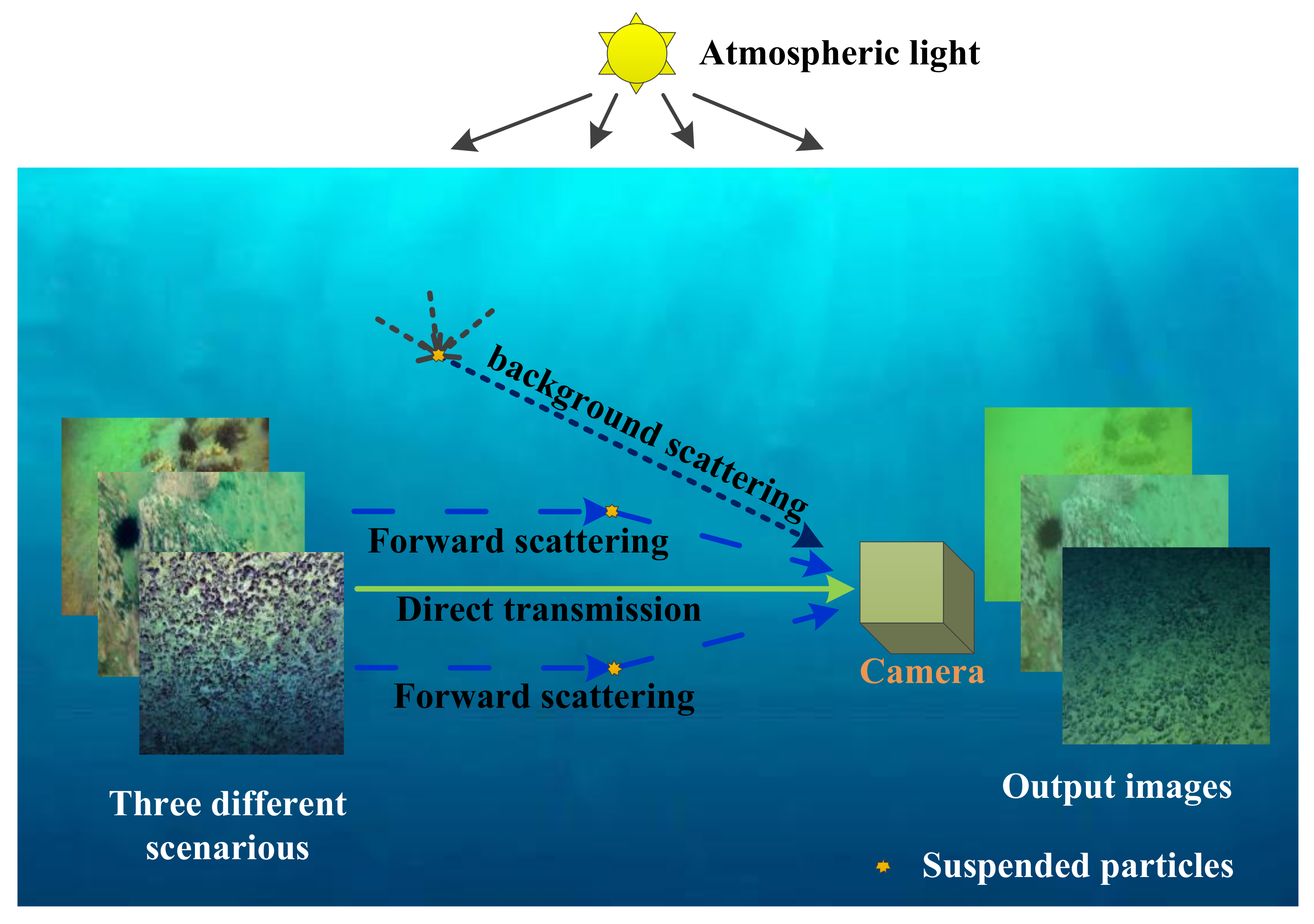
2. Background and Related Work

This section surveys the underwater imaging formation model and reviews the main methods that have been proposed to estimate the TM. The Jaffee–McGlamery model, as an underwater imaging formation model, was proposed in [22,23], and the corresponding underwater optical imaging process is shown in Figure 1. This model considers that the total irradiance ($E_T$) of the image is composed of three components: direct transmission ($E_d$), forward scattering ($E_{fs}$), and background scattering ($E_{bs}$). The model is given as:

$$E_T=E_d+E_{fs}+E_{bs}$$

(1)

where $E_d$ is the light that directly enters the camera after being reflected by the scene, $E_{fs}$ is the light that is scattered by the suspended particles after being reflected by the scene, and $E_{bs}$ represents the background light that enters the camera after being scattered by suspended particles and organics.

According to the Lambert–Beer law, the propagation of light in the medium decays exponentially. Hence, the TM ($t^c$) of light in the water can be written as:

$$t^c=e^{-a_{c}d}{e}^{-b_{c}d}=e^{-(a_c+b_c)d}=e^{-{\eta }_{c}d},c\in (R,G,B)$$

(2)

where $a_c$ and $b_c$ are respectively the absorption coefficient and the scattering coefficient, ${\eta }_c$ represents the attenuation coefficient of seawater on different channels, d is the distance from the point in the scene to the camera, and c is one of the red, green, or blue channels.

Following the nomenclature used in [24,25], $E_d$, $E_{fs}$, and $E_{bs}$ are respectively written as:

$$E_d=J^c{e}^{-{\eta }_{c}d}=J{t}^c$$

(3)

$$E_{fs}=E_d*g_d$$

(4)

$$E_{bs}=A^c(1-e^{-{\eta }_{c}d})=A^c(1-t^c)$$

(5)

where $J^c$, $g_d$, and $A^c$ are the undegraded image, point spread function, and global light, respectively; “*” represents the convolution operation. Since the distance between the camera and the underwater scene is relatively short, the degradation of underwater image caused by forward scattering can be ignored. The underwater imaging model (1) can be simplified as:

$$I^c\left(x\right)=J^c\left(x\right)t^c\left(x\right)+A^c(1-t^c\left(x\right))$$

(6)

where $I=E_T$ is the image obtained under the water and x represents the coordinates of each pixel in the image. This simplified model (6) is valid under the assumption that the medium is homogeneous. The undegraded image $J^c$ can be expressed as:

$$J^c\left(x\right)=\frac{I^c\left(x\right)-A^c}{t^c\left(x\right)}+A^c$$

(7)

From Equation (7), the undegraded image $J^c$ can be restored from $I^c$ when global light $A^c$ and $t^c$ are known.

Many methods for estimating the TM have been proposed [18,26,27,28], among which the DCP method is the most widely used method. The DCP method is a statistical prior, which is based on the observation that haze-free outdoor images have a very low intensity (close to zero) in at least one color channel in a square patch. The formulation of the dark channel image $J^{dark}$ can be defined as:

$$J^{dark}\left(x\right)=\underset{y\in \mathsf{\Omega }\left(x\right)}{min}(\underset{c\in (R,G,B)}{min}{J}^c\left(y\right))\to 0$$

(8)

where $\mathsf{\Omega }\left(x\right)$ is a local patch centered at pixel x. Taking the minimum operation of Equation (6), the TM can be expressed as:

$$\tilde{t}\left(x\right)=1-\underset{y\in \mathsf{\Omega }\left(x\right)}{min}(\underset{c\in (R,G,B)}{min}\frac{I^c\left(y\right)}{A^c})$$

(9)

During the propagation of light in water, the attenuation of red light becomes serious with the increase of the water depth. If the dark channel is directly used to estimate the TM, the red color channel will then be most likely used as the dark channel, and the expected effect cannot be achieved. After analyzing the characteristics of underwater images, some TM estimate methods were proposed for underwater images. Paulo et al. [16] basically considered that the blue and green color channels were the underwater visual information source, which means changing $c\in (R,G,B)$ in Equation (9) to $c\in (G,B)$. The TM can be estimated by Equation (10). This method seems sound and can produce good results. However, the assumption of Equation (8) will not hold due to the exclusion of the red color channel. In [17], Galdran et al. applied the inverse of the red color channel to estimate the TM of the red color channel. Meanwhile, the TM of the blue color channel and the green color channel were estimated by Equation (2), respectively. Furthermore, the paper [29,30] estimated the TM of different channels from the perspective of light attenuation. However, since the estimated TM has block-like artifacts using the above methods, it needs to be fine-tunedby guided filtering [20] or soft matting [21]. The fine-tuningoperation of those methods results in a large calculation cost. Hence, this paper proposes an underwater image restoration method with transmission estimation using color constancy, which directly derives the TM by calculating the illumination component of the red channel, blue channel, and green channel of the initial image, respectively. The results of the underwater image restoration using the above methods are shown in Figure 2.

It can be seen from Figure 2 that the underwater image restoration methods developed in [16,28,29] have a certain degree of restoration performance on the second row of images, but they are basically ineffective for images with bluish-green tones (the first row). Compared with these methods, the proposed method in Section 2 of this paper can adapt to the two different underwater scenes. Later in this paper, Section 3 will present other examples and methods and quantitatively analyze the restoration performances of these methods on underwater images.

$$\tilde{t}\left(x\right)=1-\underset{y\in \mathsf{\Omega }\left(x\right)}{min}(\underset{c\in (G,B)}{min}\frac{I^c\left(y\right)}{A^c})$$

(10)

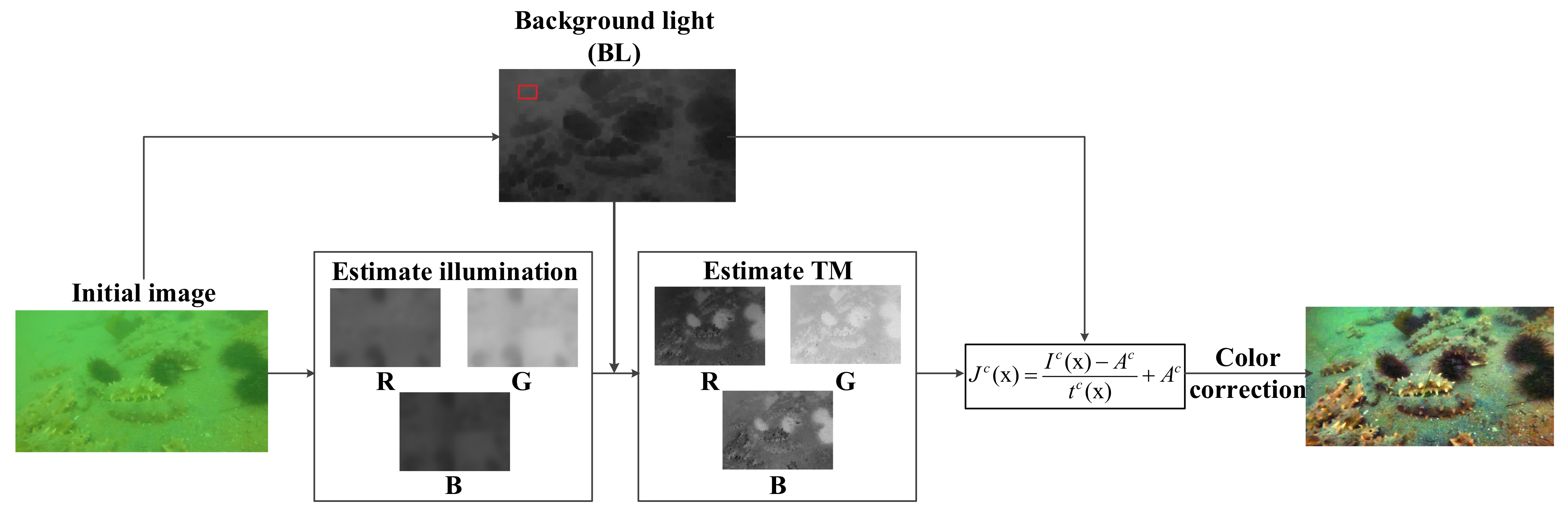
3. The Color-Constancy-Based Underwater Image Restoration Method

To suppress the color distortion and blurring of underwater images, this paper proposes a new underwater image restoration method with TM estimation using color constancy. The proposed underwater restoration method involves four main steps: estimate the BL, estimate the illumination, estimate the TM with color constancy, and color correction. The flowchart of the proposed underwater image restoration method is shown in Figure 3. The estimation method of background light (A) in the proposed method comes from the UDCP method, which first picks the top 0.1% brightest pixels in the dark channel of the blue and green channels, and then, the highest intensity of these pixels in the raw image is selected as the background light.

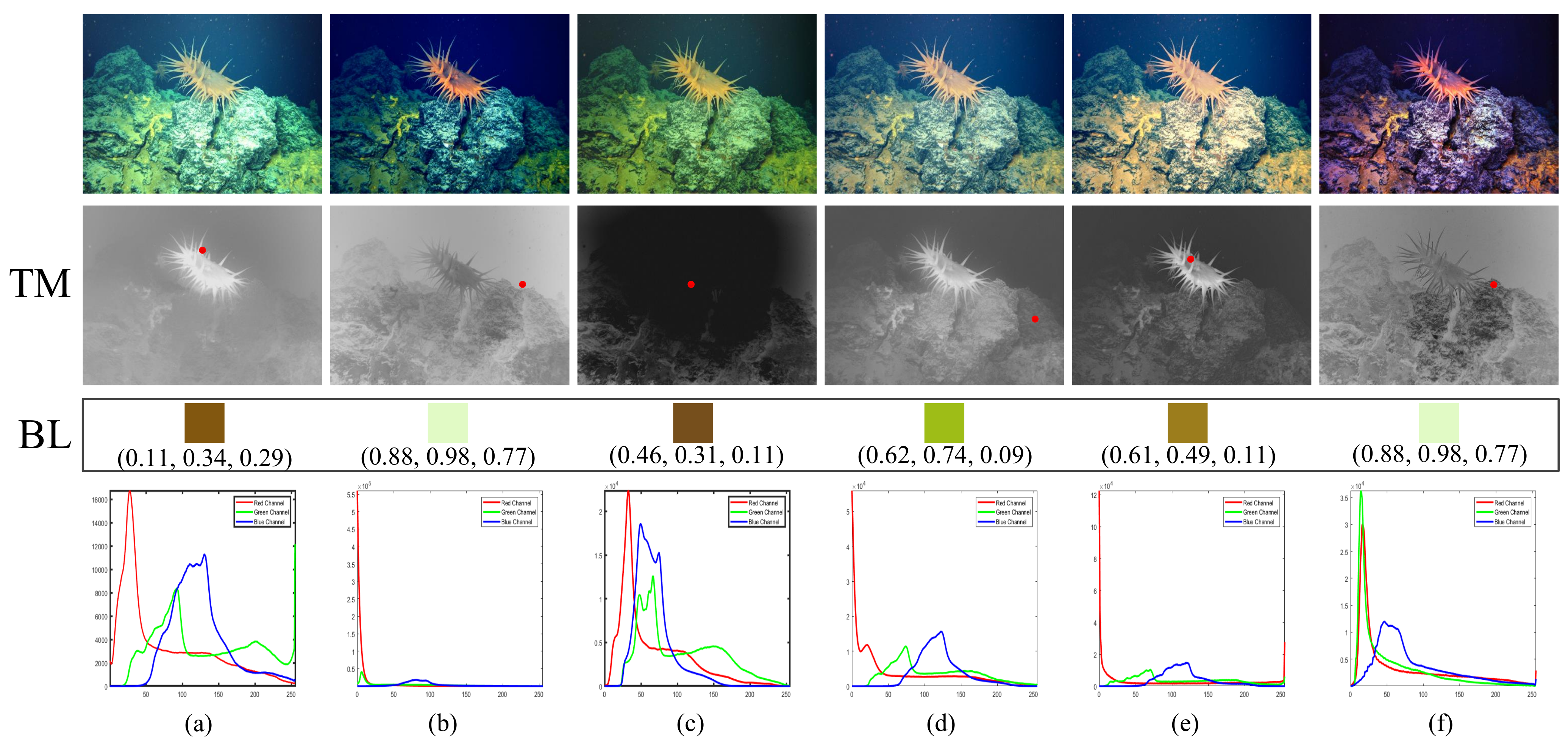
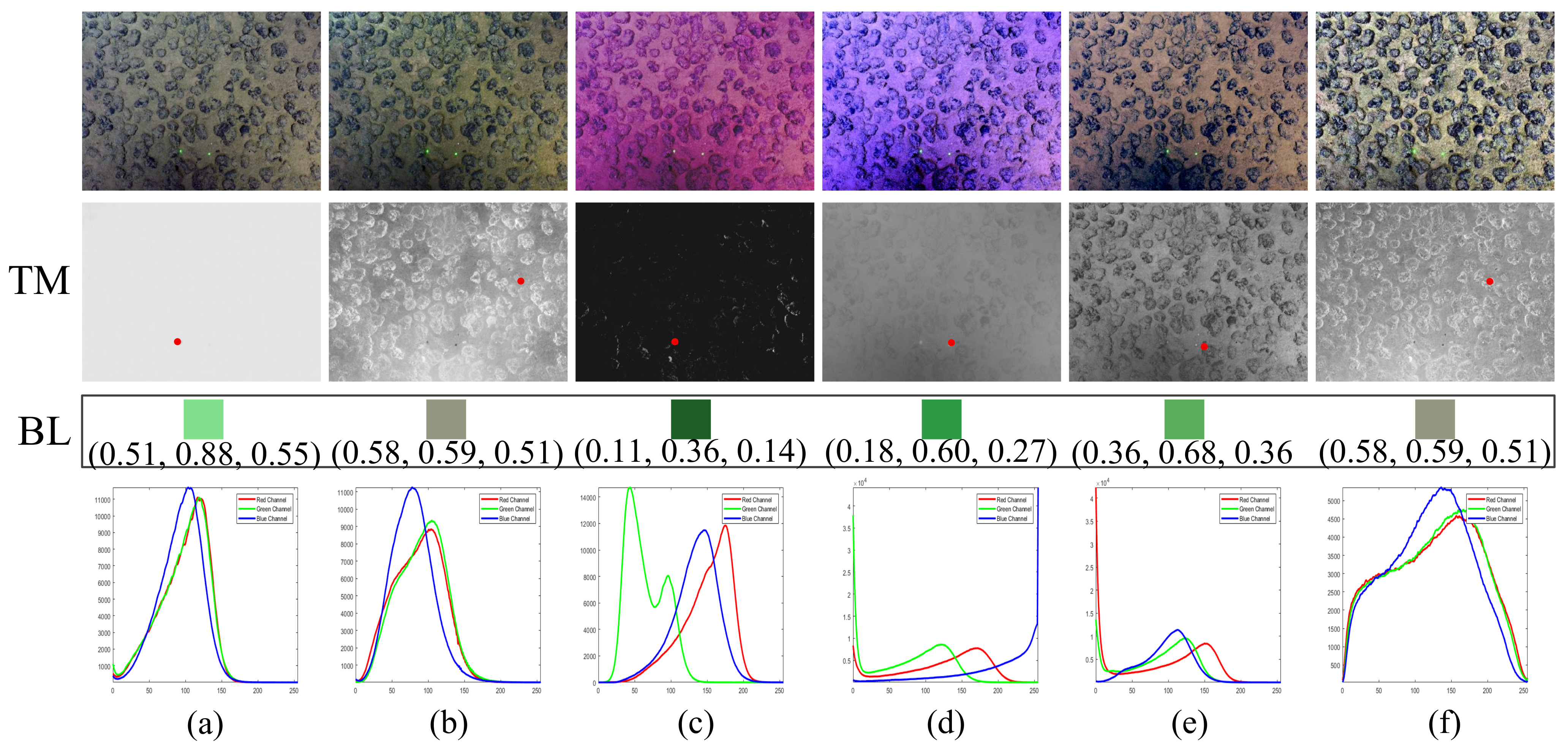
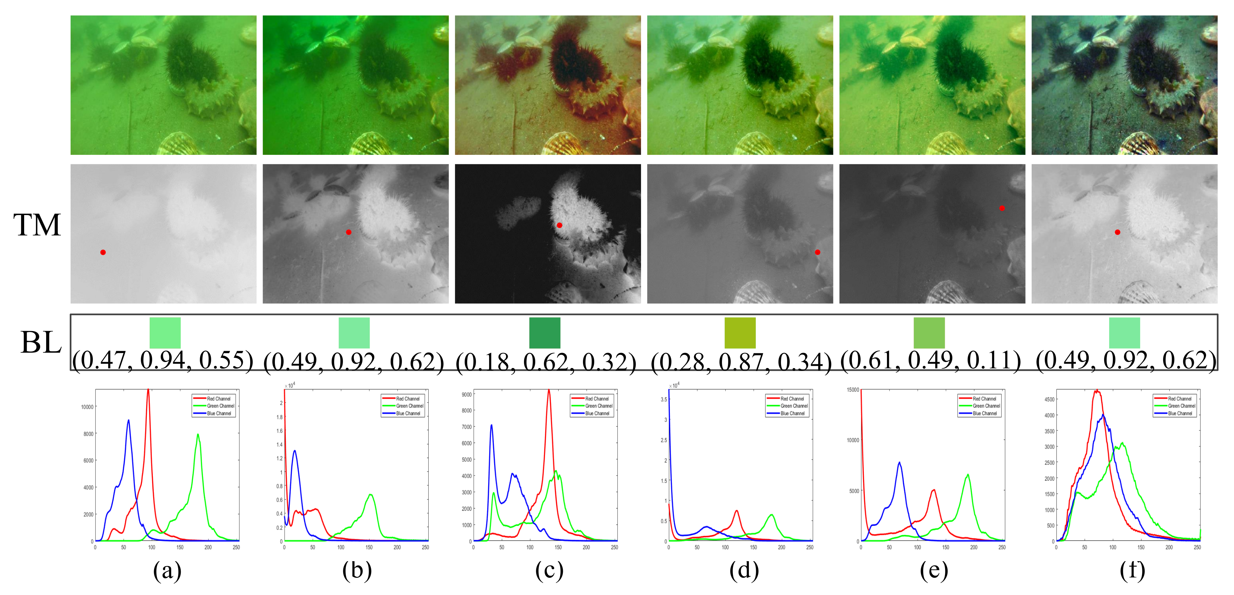
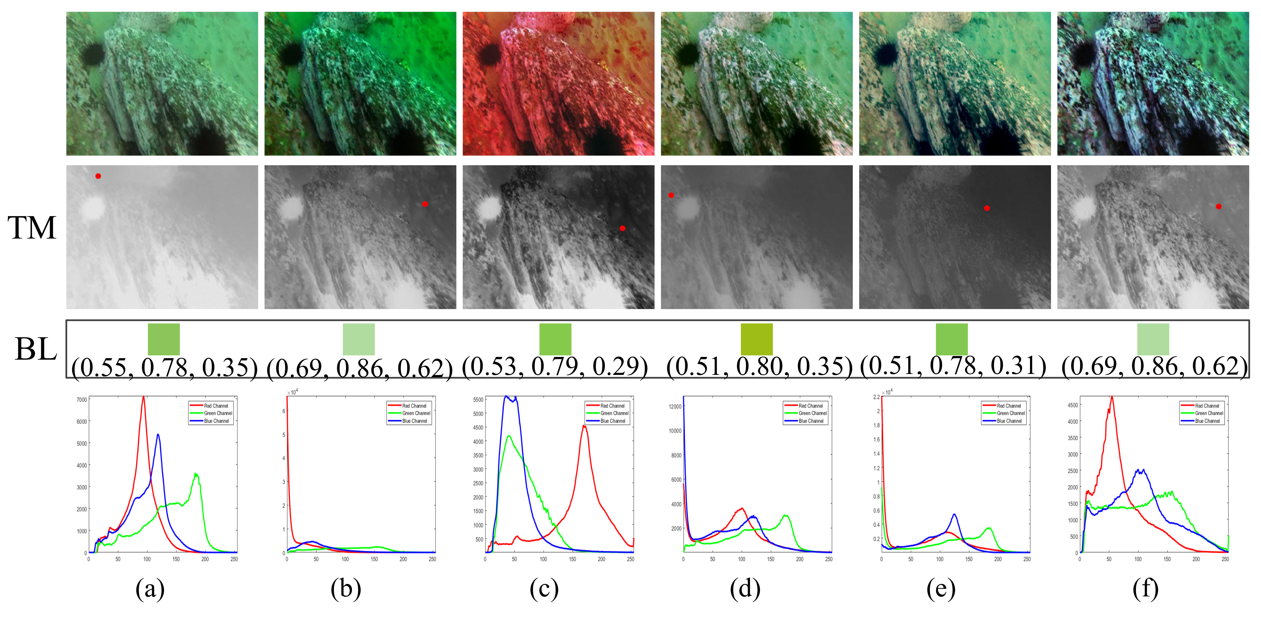
3.1. The Spatial Distribution of the Source Illumination Based on Color Constancy

According to Land’s retinex theory, the object color is determined by its own reflection ability and cannot be affected by the uneven illumination, which is called the color constancy. The spatial distribution of the illumination of each channel can be estimated by calculating the weighted average of a pixel point and the pixel points in its surrounding area in the image. The spatial distribution of the source illumination is described as:

$$L^c\left(x\right)=I^c\left(x\right)*F(m,n,\sigma )$$

(11)

where I is the image obtained under water and $x=(m,n)$ represents the coordinates of an individual image pixel, where m and n respectively represent the vertical and horizontal coordinates of the pixel, L is the spatial distribution of the source illumination, “*” represents the convolution operation, c presents one of the red, green, or blue channels, and $F(m,n,\sigma )$ is the Gaussian surround function, defined in the following way:

$$F(m,n,\sigma )=\lambda e^{(-(m^2+n^2)/2{\sigma }^2)}$$

(12)

$\lambda$ is the normalization scale so that $\int \int F(m,n,\sigma )dmdn=1$ and $\sigma$ is the Gaussian surround scale. The value of $\sigma$ has different effects on the contrast and color distortion of the restored images. The details of the dark area in the image can be better enhanced by the small value of $\sigma$, and the chroma consistency of the image is better kept by the large value of $\sigma$. To this end, in this section, inspired by [31], the multi-scale Gaussian surround function is used to acquire the spatial distribution of the source illumination. Hence, Equation (11) can be written as:

$$L^c\left(x\right)={\displaystyle \sum _{k=1}^{N_k}}{\omega }_k{I}^c\left(x\right)*F(m,n,{\sigma }_k)$$

(13)

where $N_k$ is the number of scales and ${\omega }_k$ represents the weight coefficient of the scale, which needs to satisfy ${\displaystyle \sum _{k=1}^{N_k}}{\omega }_k=1$. The general parameter settings are as follows: $N_k=3$, ${\omega }_1=0.5$, ${\omega }_2=0.4$, ${\omega }_3=0.1$, ${\sigma }_1=15$, ${\sigma }_2=80$, and ${\sigma }_3=200$.

3.2. TM Estimation with the Illumination Spatial Distribution Color Constancy

From Section 1, the TM estimation of some DCP-based methods (e.g., [16,17]) will not hold the assumption of Equation (8). In order to ensure the validity of the assumption of Equation (8), in this section, the estimation of the TM with the illumination spatial distribution using the color constancy is performed.

In retinex, the illumination spatial distribution is used to compute the reflected image of the scene. The retinex model can be described as:

$$I^c\left(x\right)=R^c\left(x\right)L^c\left(x\right)$$

(14)

where $R\left(x\right)$ is the reflected image of the scene, which represents the undegraded image. $I\left(x\right)$ represents the initial image. Meanwhile, $J\left(x\right)$ also represents the undegraded image in Equation (6). Therefore, it is reasonable to assume that $R\left(x\right)=J\left(x\right)$. Combining Equations (6) and (14), a novel underwater optical imaging model can be written as:

$$I^c\left(x\right)=\frac{A^c(1-L^c\left(x\right))t^c\left(x\right)}{L^c\left(x\right)-t^c\left(x\right)}+A^c$$

(15)

The TM (i.e., $t^c\left(x\right)$) can be accurately estimated from $I^c\left(x\right)$ when the BL (i.e., $A^c$) and the spatial distribution of the source illumination (i.e., $L^c\left(x\right)$) are known. Therefore, the TM can be derived as:

$$t^c\left(x\right)=\frac{(I^c\left(x\right)-A^c)L^c\left(x\right)}{I^c\left(x\right)-A^c{L}^c\left(x\right)}$$

(16)

With the TM (i.e., $t^c\left(x\right)$) of each channel of the initial image $I\left(x\right)$, the undegraded image $J\left(x\right)$ can be obtained according to Equation (7).

3.3. Color Correction

Typically, the distribution of pixels is severely unbalanced in different channels of the underwater images. When transmitting through the water, the long-wavelength light is absorbed faster than the short-wavelength light. Due to the light propagation characteristics in the water, the underwater images are always dominated by the cyan tone. Although the image restoration method proposed in this section suppresses the color shift to a great extent, there is still a lack of sufficient overall brightness. Moreover, the pixel values of the restored image do not satisfy 0–255. Therefore, one color correction algorithm was designed to fine-tune the color unbalance of the underwater images based on the statistical property of the pixel. The color correction algorithm is given as follows:

$$J^c\left(x\right)=\frac{J^c\left(x\right)-min\left(J^c\left(x\right)\right)}{max(J^c\left(x\right)-min\left(J^c\left(x\right)\right))},c\in (R,G,B)$$

(17)

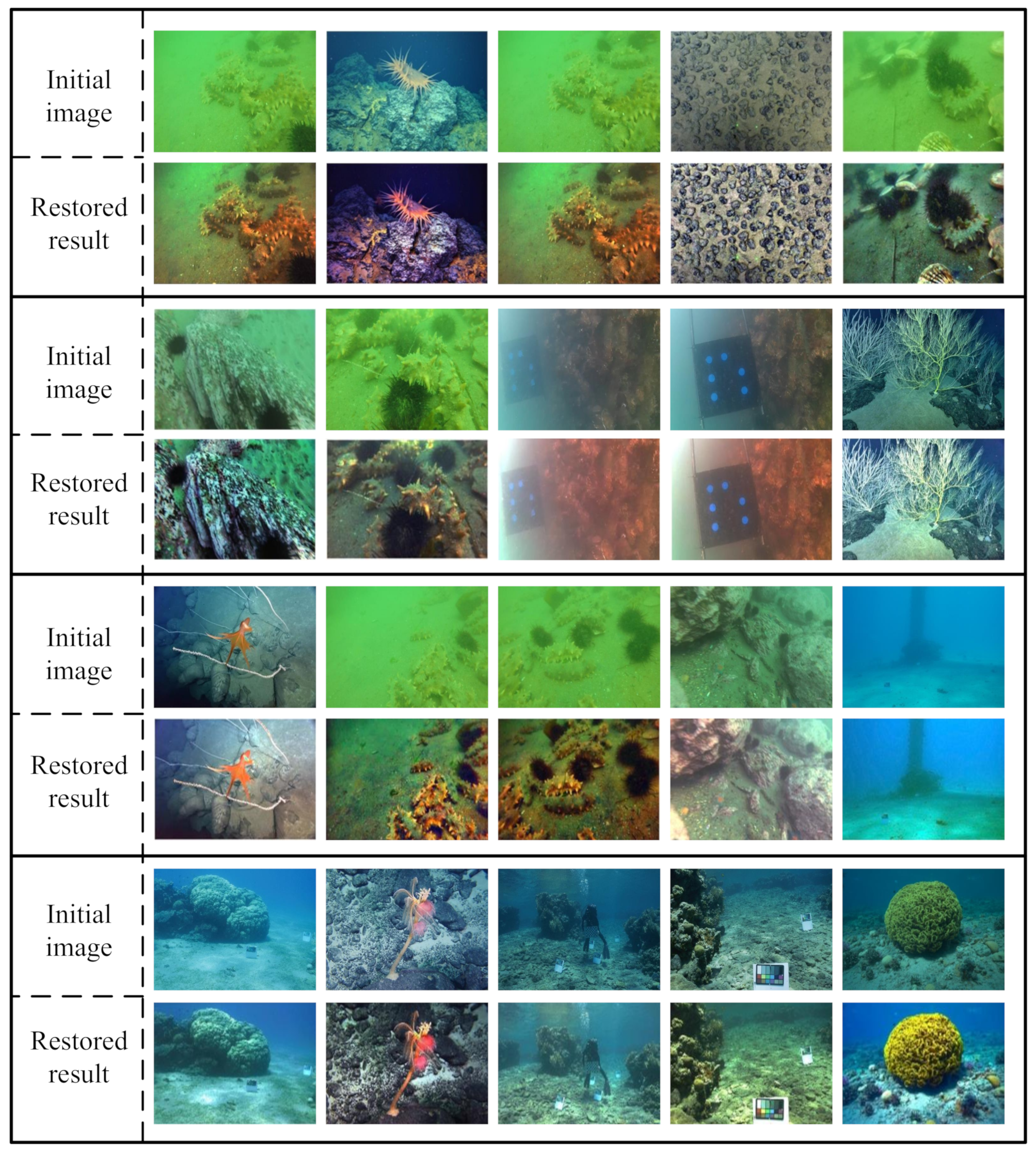
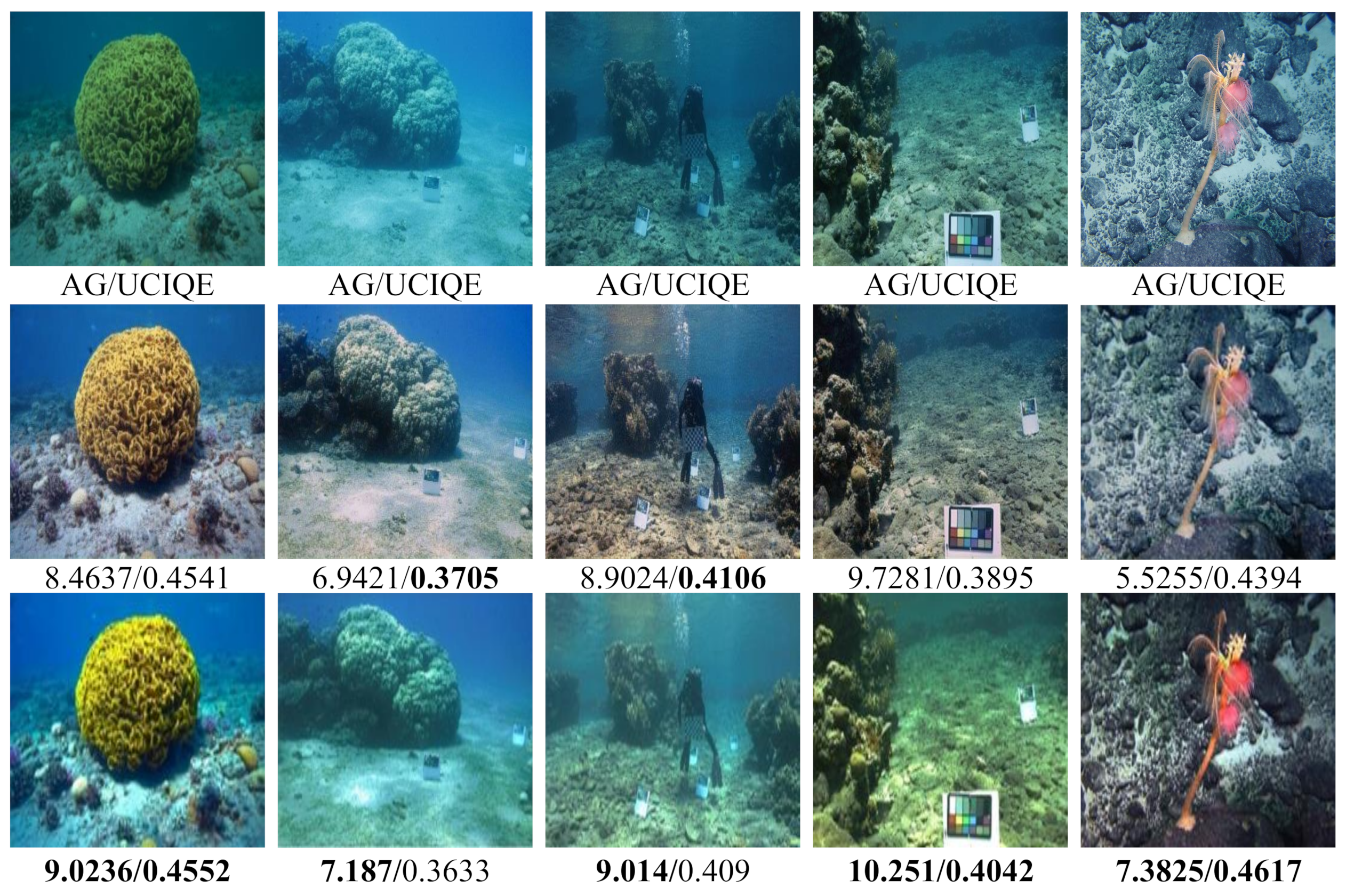
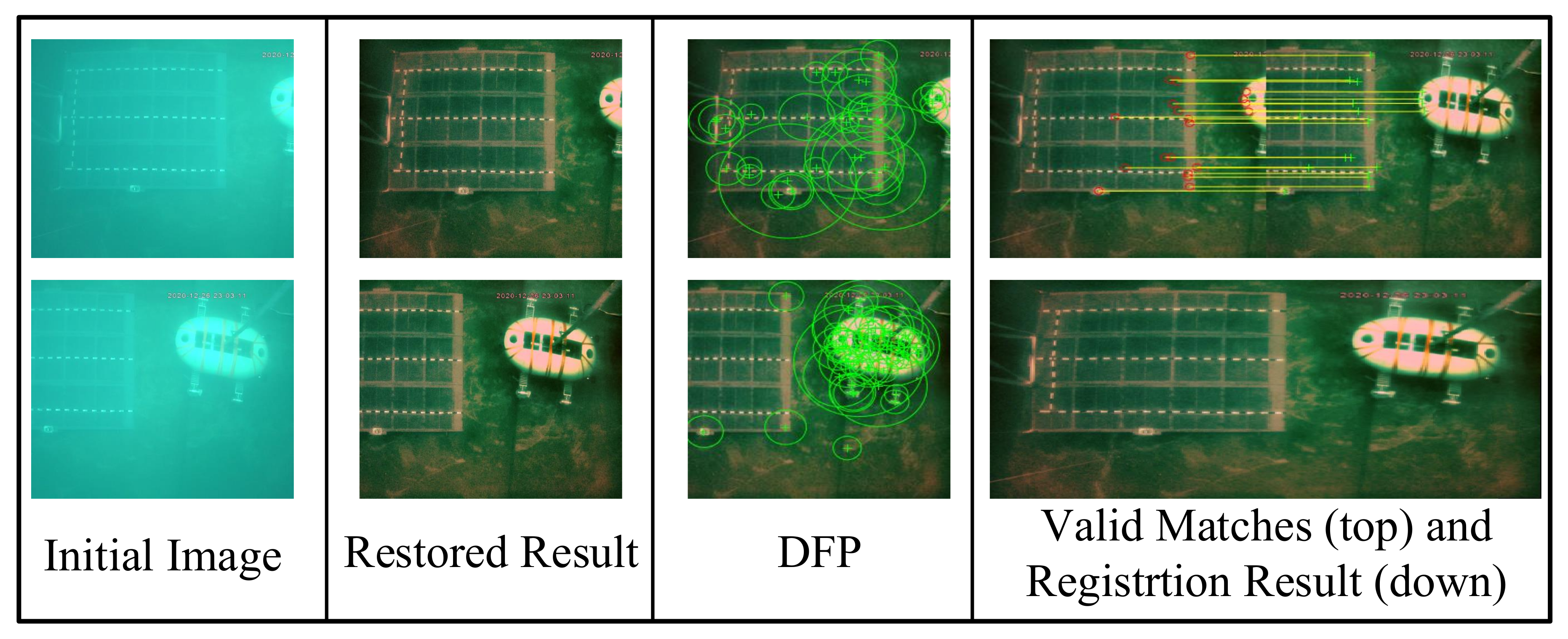
4. Experimental Results

In this section, in order to verify the efficiency of the proposed algorithm in this paper, the qualitative comparison and the quantitative comparison are implemented, respectively. There are four underwater images with different scenes shown in Figure 4 to be use for testing. These images mainly came from two places: real underwater images of the Western Pacific (Figure 4a,b) and the dataset of the China 2019 Underwater Object Detection Algorithm Contest (Figure 4c,d). All experiments were performed using MATLAB 2016b on a Windows 7 PC with Intel(R) Core(TM) i5-3210M CPU at 2.50 GHz and 4.00 GB RAM.

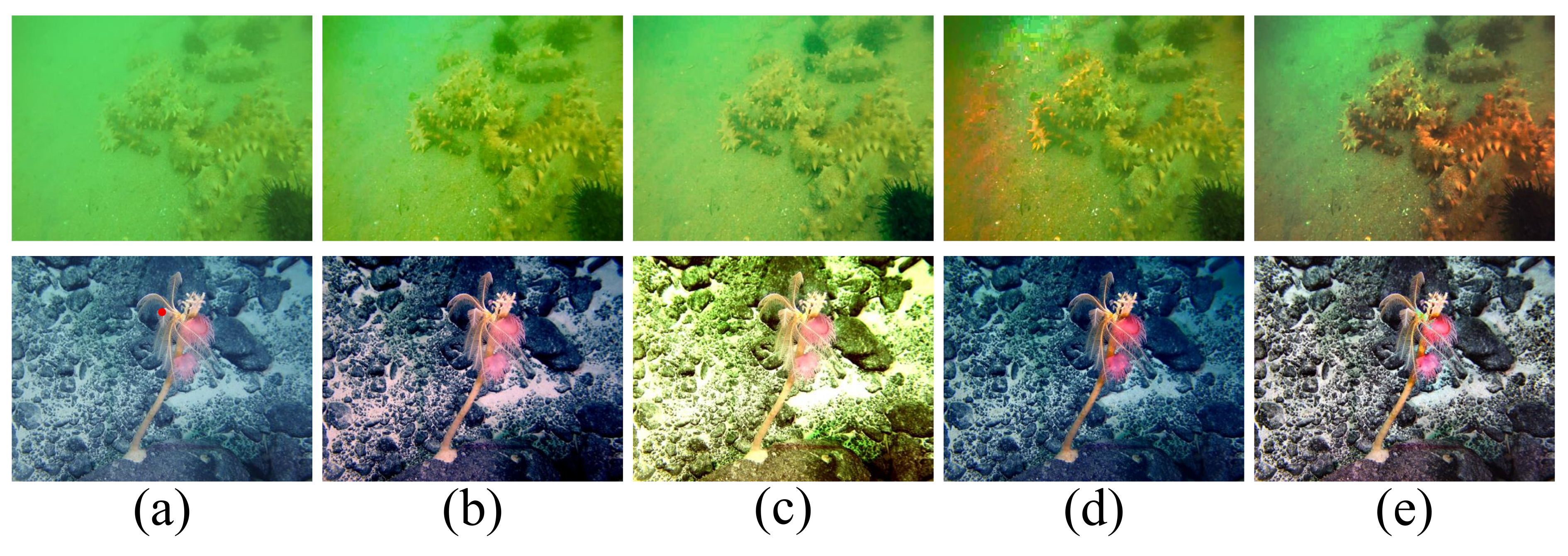
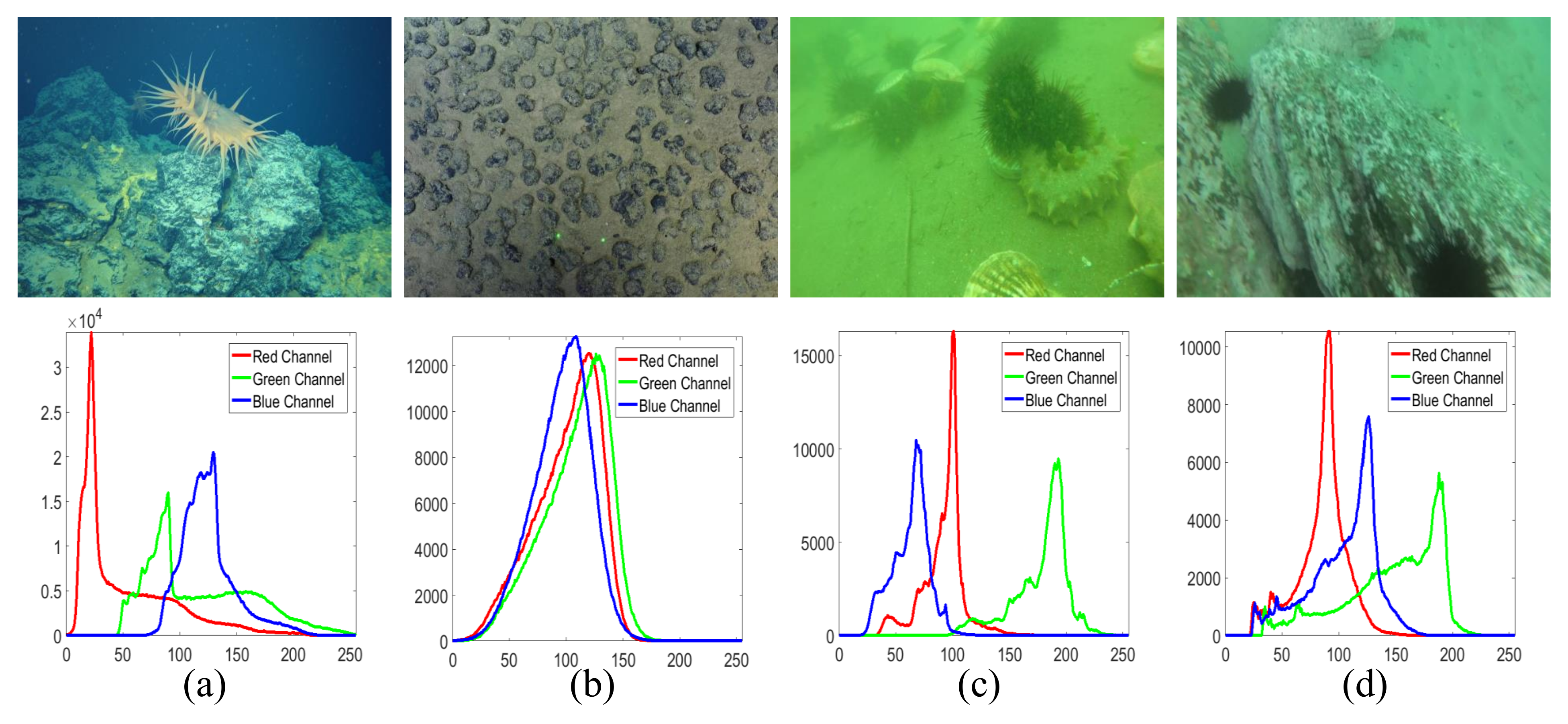
4.1. Qualitative Comparison

In this part, the proposed underwater image restoration method is compared with other state-of-the-art methods including the maximum intensity prior (MIP) method [28], the underwater dark channel prior (UDCP) method [16], Li’s method [32], Peng’s method (IBLA) [29], and the underwater light attenuation prior (ULAP) method [30].

In Figure 5, the light distribution is uneven in the initial image (Figure 4), which has some bright pixels in the foreground and dark pixels in the background. The restoration result based on the MIP method had local overexposure, which was caused by the large TM. The TM was estimated by the difference between the maximum red channel intensity and the maximum intensity of the green and blue channels. Even though the TM was properly estimated based on the UDCP method, the restoration result was unsatisfactory because the brighter foreground made the BL detected on a rock. The wrong BL and incorrect TM estimated by the hierarchical searching technology depending on the degraded channel led to the failure of Li’s method for this case. The results from the IBLA and ULAP methods looked more significant, which indicates that the non-uniform illumination underwater image can be restored well using the light attenuation prior and the blurred information of the original image. The proposed method estimated a proper TM in this case, but gave an overall dimmer restoration result due to the fact that the brighter foreground caused the wrong estimation of the BL. However, the proposed method can better reflect the real tones of the object in terrestrial images, such as the color of stones being black instead of blue or green.

In contrast, the initial image in Figure 4b is dimly lit and has two distinct green spots. It can be seen from the comparison results in Figure 6 that the above methods cannot work for this case except the ULAP and the proposed method. The results from the MIP method, the IBLA method, and Li’s method look insignificantly restored because of the incorrect TM and wrong BL estimation. Furthermore, the red channel is used in Li’s method to perform color correction, and consequently, the restored image had a red tone. The BL and TM estimated by the image blur was insufficient for this case; therefore, the restored image had a color shift using the IBLA method (the restored image showed a purple tone). The UDCP method can restore the initial image to a certain extent, but the background of the restored image was darker due to the lack of the red channel information. For the ULAP method, even though the TM was correctly estimated, it had an unsatisfactory restoration result due to the Wang estimation of the BL. Compared with the ULAP method, the restoration result obtained by the proposed method had better contrast, saturation, and brightness.

Figure 7 gives the result of restoring a greenish underwater image, whose red channel is severely attenuated. The restored image obtained by the MIP method and the UDCP method hardly was affected because they only estimate one single TM without considering different attenuation levels for the RGB channels, although they can correctly estimate the BL. Li’s method not only selected the wrong BL, but estimated an incorrect TM and failed to restore the image. The fogging phenomenon and the scene edge can be improved to a certain extent by the IBLA and ULAP methods, but the restored images were still bluish in tone due to the darkness of the estimated TM. For this case, the method proposed in this paper estimated the BL and TM more accurately, which enhanced the details of the scene edge while eliminating the color distortion.

Lastly, Figure 8 demonstrates the result of restoring the bluish underwater image shown in Figure 4d. All methods worked well for this case except Li’s method, and the obtained images all looked restored and enhanced, although some color differences existed. The reason for the red distortion in the restored image from Li’s method was because of the red channel color correction based on adoption of the gray world hypothesis. From the comparison results of the above methods in this case, the proposed method can obtain more accurate BL and TM, and the restored image had a satisfactory recovery effect.

Furthermore, the distribution histograms of the R, G, and B channels of four initial underwater images of Figure 4 presented in the last row of Figure 4 and the corresponding results after using the MIP [28], UDCP [16], Li’s method [32], IBLA [29], ULAP [30], and the proposed method are displayed in order in the last row of Figure 5, Figure 6, Figure 7 and Figure 8 (the x-axis represents the signal levels; the y-axis represents the normalized frequency). As shown in these distribution histograms, the histogram distribution of the RGB channels of the restored images using the proposed method were wider and more uniform. Combined with the restoration results, the proposed underwater image restoration method can obtain restored images with higher contrast and clearer details.

4.2. Quantitative Comparison

In order to further verify the efficiency of the underwater image restoration method proposed in this paper, this section compares the proposed method with aforementioned methods using several objective metrics to conduct a quantitative analysis. Considering the aspects of the information richness, naturalness, sharpness, and overall index of contrast, chroma, and saturation, four evaluation metrics, namely the average gradient (AG), the entropy, the contrast restoration, and the underwater color image quality evaluation metric (UCIQE), were chosen to comprehensively evaluate the restoration effect. The AG was used to assess the image clarity, where a larger value of the AG means a clearer image. The entropy represents the amount of information contained in the image, which can reflect the resolution of the scene details. The higher the entropy value, the better the quality of the image will be and the clearer the image will be. The contrast can represent the restored quality of the contrast after employing the underwater image restoration method. The bigger the value is, the better the dehazing is. The UCIQE was developed to reflect the quality of underwater color images, and it is calculated a a linear model of the contrast of the image brightness, the standard deviation of the image chromaticity, and the average of the image saturation in the CIE-Lab color space. The UCIQE is a comprehensive evaluation index. The larger the UCIQE value is, the better the underwater color image quality will be. The value of these metrics is respectively defined as Equation (18):

$$\begin{gathered} \left\{\begin{array}{c}AG=\frac{1}{M\times N}\sum _{x,y}\sqrt{(d{I}_x^2+d{I}_y^2)/\phantom{(d{I}_x^2+d{I}_y^2)2}2}\\ \\ Entropy=-{\displaystyle \sum _{i=0}^L}{p}_i{log}_2{p}_i\\ \\ Contract=\sum _{\delta }{\delta }_{(i,j)}^2{p}_{\delta (i,j)}\\ \\ UCIQE=c_1\times {\sigma }_c+c_2\times co{n}_l+c_3\times {\mu }_s\end{array}\right. \end{gathered}$$

(18)

. where $(x,y)$ represents the pixel coordinates of the image, $d{I}_x$ and $d{I}_y$ are respectively the partial derivatives of x and y, $M\times N$ is the size of the image, $p_i$ is the normalized frequency of the gray value i, $L=255$ represents the gray level, ${\delta }_{(x,y)}$ is the grayscale difference between adjacent pixels, $p_{\delta (x,y)}$ represents the probability of the pixel distribution that the grayscale difference between adjacent pixels is $\delta$, ${\sigma }_c$, $co{n}_l$, and ${\mu }_s$ represent the standard deviation of the image chromaticity, the contract of the image brightness, and the average of the image saturation, respectively, and $c_1$, $c_2$, and $c_3$ are three constant coefficients, typically taken as $c_1=0.4680$, $c_2=0.2745$, and $c_3=0.2576$.

Table 1. Quantitative analysis of the restoration results based on different methods (the bold values express the best metric values).

Initial Images	MIP [28]				UDCP [16]				Li’s Method [32]
	AG	Entropy	Contrast	UCIQE	AG	Entropy	Contrast	UCIQE	AG	Entropy	Contrast	UCIQE
$\left(a\right)$	7.8452	16.3016	50.9766	0.4197	6.4357	14.1648	31.9105	0.5167	5.6237	15.1937	36.1423	0.4171
$\left(b\right)$	8.4506	13.9274	23.8966	0.3196	8.8771	15.7372	24.3995	0.3073	8.0575	15.5760	22.0549	0.3406
$\left(c\right)$	1.7832	12.6811	16.4860	0.3450	1.8808	14.4660	12.6179	0.4129	2.8828	14.6900	27.8984	0.3909
$\left(d\right)$	4.0887	14.6109	28.5579	0.3334	4.7030	15.8857	25.0513	0.4542	4.9687	15.2902	24.0916	0.5078
Average	5.5419	14.3802	19.9792	0.3544	5.4742	15.0634	23.4948	0.4228	5.3832	15.1875	27.5468	0.4141

and

Table 2. Quantitative analysis of the restoration results based on different methods (the bold values express the best metric values).

Initial Images	IBLA [29]				ULAP [30]				The Proposed Method
	AG	Entropy	Contrast	UCIQE	AG	Entropy	Contrast	UCIQE	AG	Entropy	Contrast	UCIQE
$\left(a\right)$	6.6599	15.7478	44.1143	0.4152	8.4623	15.8384	56.6435	0.4617	9.7705	16.7100	37.4011	0.5085
$\left(b\right)$	13.0467	16.0884	36.0871	0.4281	11.2939	14.9631	34.5920	0.4436	20.6358	17.7885	49.8168	0.4172
$\left(c\right)$	2.7248	14.3524	26.4115	0.4224	2.7956	14.2086	26.8171	0.4018	4.6639	16.1528	26.7410	0.3879
$\left(d\right)$	6.1937	15.9053	37.2614	0.3972	6.1703	15.6731	39.9646	0.4031	8.5353	16.8028	39.7184	0.4331
Average	7.1563	15.5235	35.9686	0.4157	7.1805	15.1708	39.5043	0.4276	10.9014	16.8635	38.4193	0.4367

show the AG, entropy, contract, and UCIQE values of the restored images of the above methods. The best results are highlighted in bold. The AG and entropy values of the proposed method were generally higher than those of the restored images by other methods. This suggests that the proposed method can improve the information abundance and sharpness contained in the image. Although the contrast of the restoration images of Figure 4c and the UICQE values of the restoration images of Figure 4d obtained by Li’s method were the highest, the restored images appeared unnatural, according to Figure 7c and Figure 8c. This was because the restored images obtained by Li’s method had the highest standard deviation of image chromaticity. These restored images had high metrics using the IBLA method, but the restoration result in Figure 4b is obviously poor, which was caused by a lack of brightness in the initial image. The ULAP method obtained relatively higher score of some metrics and achieved good image restoration in some scenes. By contrast, although the UCIQE metric of the proposed method was not the highest in each image in Figure 4, the average value of the UCIQE metric reached by the method proposed in this paper was the highest. This shows that the proposed method in this paper has better average performance.

Meanwhile, we selected 150 underwater test images with a size of $720\times 450$ from several datasets for statistical analysis. Their average processing time and standard deviation are presented in

Table 3. The average processing time and standard deviation of different methods (the bold values express the best metric values).

Methods	MIP [28]	UDCP [16]	Li’s Method [32]	IBLA [29]	ULAP [30]	The Proposed Method
Processing time(s)	13.2412	17.5264	21.3852	43.0186	4.3546	4.1124
Standard Deviation	0.2152	0.3354	0.2541	0.2285	0.2737	0.2017

.

Table 4. Average values of 4 quantitative evaluation metrics for the 150 underwater test images (the bold values express the best metric values.)

Methods	MIP [28]	UDCP [16]	Li’s Method [32]	IBLA [29]	ULAP [30]	The Proposed Method
AG	6.3825	6.1311	5.0623	9.2365	9.4357	11.9822
Entropy	13.7691	15.4799	15.3824	16.0378	15.9395	16.3776
Contrast	37.4366	21.1347	26.1455	39.4728	42.1598	41.7541
UCIQE	0.3123	0.3977	0.4035	0.4157	0.4266	0.4314

reports the statistical results of different methods in terms of the AG, entropy, contrast, and UCIQE for the 150 underwater test images. From Table 3, it can be seen that the average processing time for the IBLA reached 43.0186 s, which is obviously not suitable for real-time underwater applications. The average processing time of the proposed method in this paper was 4.1124 s, which is basically the same as the processing times of the ULAP method. Meanwhile, the standard deviation of the proposed method was relatively small. It can be seen from Table 4 that all metrics obtained by the proposed method in this paper except the contrast were improved to varying degrees. Although the contrast of the proposed method was not the highest, it reached the second highest of all the methods. Besides, the restoration results of the 20 underwater test images (randomly selected from the 150 underwater test images) by the proposed method are shown in Figure 9. Combining Figure 9 and Table 4, we can conclude that the proposed method in this paper can reduce the processing time while ensuring the image restoration effect.

Furthermore, to further analyze the effectiveness of the method proposed in this paper, we compared it with DUIENet [33], which is a CNN-based underwater image restoration method. Figure 10 shows some test results. The AG and UCIQE were chosen to comprehensively evaluate the restoration effect. As can be seen from Figure 10, compared with DUIENet, the method proposed in this paper had a good effect in suppressing blur and color distortion and had better index parameters.

Local feature point matching is a fundamental task in many computer vision applications [34]. The scale-invariant feature transform (SIFT) is a scale-invariant local feature descriptor that can detect key points in the images. To prove the effectiveness of the proposed method in this paper for image matching tasks, the SIFT operator was applied to compute the keypoints. The local feature point matching results of a pair of underwater images and that of the corresponding pair of images restored by the proposed underwater image restoration method are displayed in Figure 11. The promising results presented in Figure 11 demonstrate that the restored images using the proposed method in this paper had an increased number of matched pairs of feature points. This is very helpful for underwater image recognition and matching tasks.

5. Conclusions

This paper proposed a new underwater image restoration method with transmission estimation using color constancy. The transmission map was estimated by using the illumination component of the initial image instead of using the DCP or MIP, which can avoid the large processing time caused by guided filtering or soft matting and can improve the real-time performance. Furthermore, the statistical properties of the pixels were used to fine-tune the pixel distribution of each channel because of the uneven distribution of the pixel values in the restored image. Both the qualitative and quantitative experimental results showed that the proposed underwater image restoration method in this paper can obtain better restoration performances in different underwater scenes compared to other underwater image restoration methods.

References

1. Lu, H.; Wang, D.; Li, Y.; Li, J. CONet: A Cognitive Ocean Network. IEEE Wirel. Commun. 2019, 26, 90–96. [Google Scholar]
2. Inoue, Y.; Hisano, D.; Maruta, K.; Hara-Azumi, Y.; Nakayama, Y. Deep Joint Source-Channel Coding and Modulation for Underwater Acoustic Communication. In Proceedings of the 2021 IEEE Global Communications Conference (GLOBECOM), Madrid, Spain, 7–11 December 2021; pp. 1–7. [Google Scholar]
3. Al-Zhrani, S.; Bedaiwi, N.M.; El-Ramli, I.; Barasheed, A. Underwater Optical Communications: A Brief Overview and Recent Developments. Eng. Sci. 2021, 16, 146–186. [Google Scholar]
4. Esmaiel, H.; Qasem, Z.A.H.; Sun, H.; Wang, J.; Junejo, N.U.R. Underwater image transmission using spatial modulation unequal error protection for internet of underwater things. Sensors 2019, 19, 5271. [Google Scholar]
5. Esmaiel, H.; Jiang, D. SPIHT coded image transmission over underwater acoustic channel with unequal error protection using HQAM. In Proceedings of the 2013 IEEE Third International Conference on Information Science and Technology (ICIST), Yangzhou, China, 23–25 March 2013; pp. 1365–1371. [Google Scholar]
6. Esmaiel, H.; Jiang, D. Progressive ZP-OFDM for Image Transmission Over Underwater Time-Dispersive Fading Channels. In Proceedings of the 2018 International Conference on Computing, Electronics and Communications Engineering (iCCECE), Southend, UK, 16–17 August 2018; pp. 226–229. [Google Scholar]
7. Farhad, G.; Aria, A.; Hassan, S.; Hashemi, M.; Shahbazi, M. Model identification of a Marine robot in presence of IMU-DVL misalignment using TUKF. Ocean Eng. 2020, 206, 107344. [Google Scholar]
8. Mousavian, S.H.; Koofigar, H.R. Identification-Based Robust Motion Control of an AUV: Optimized by Particle Swarm Optimization Algorithm. J. Intell. Robot. Syst. 2017, 85, 331–352. [Google Scholar]
9. Chen, W.; Gu, K.; Lin, W.; Yuan, F.; Cheng, E. Statistical and Structural Information Backed Full-Reference Quality Measure of Compressed Sonar Images. IEEE Trans. Circuits Syst. Video Technol. 2020, 30, 334–348. [Google Scholar]
10. Lu, H.; Uemura, T.; Wang, D.; Zhu, J.; Huang, Z.; Kim, H. Deep-Sea Organisms Tracking Using Dehazing and Deep Learning. Mob. Netw. Appl. 2018, 6, 1008–1015. [Google Scholar]
11. Chen, L.; Zhou, J.; Zhao, W. A Real-Time Vehicle Navigation Algorithm in Sensor Network Environments. IEEE Trans. Intell. Transp. Syst. 2012, 13, 1657–1666. [Google Scholar]
12. Qin, H.; Yu, X.; Zhu, Z.; Deng, Z. An Expectation-Maximization Based Single-Beacon Underwater Navigation Method with Unknown ESV. Neurocomputing 2020, 378, 295–303. [Google Scholar]
13. Hou, G.; Pan, Z.; Wang, G.; Yang, H.; Duan, J. An efficient nonlocal variational method with application to underwater image restoration. Neurocomputing 2019, 369, 106–121. [Google Scholar]
14. He, K.; Sun, J.; Tang, X. Single Image Haze Removal Using Dark Channel Prior. IEEE Trans. Pattern Anal. Mach. Intell. 2011, 33, 2341–2353. [Google Scholar] [PubMed]
15. Chao, L.; Wang, M. Removal of water scattering. In Proceedings of the 2010 2nd International Conference on Computer Engineering and Technology, Chengdu, China, 16–18 April 2010; pp. 35–39. [Google Scholar]
16. Paulo, D., Jr.; Nascimento, E.; Moraes, F.; Botelho, S.; Campos, M. Transmission Estimation in Underwater Single Images. In Proceedings of the IEEE International Conference on Computer Vision (ICCV) Workshops, Sydney, Australia, 2–3 December 2013; pp. 825–830. [Google Scholar]
17. Galdran, A.; Pardo, D.; Picón, A.; Alvarez-Gila, A. Automatic Red-Channel underwater image restoration. J. Vis. Commun. Image Represent. 2015, 26, 132–145. [Google Scholar]
18. Peng, Y.; Cao, K.; Cosman, P.C. Generalization of the Dark Channel Prior for Single Image Restoration. IEEE Trans. Image Process. 2018, 27, 2856–2868. [Google Scholar] [PubMed]
19. Hou, G.; Li, J.; Wang, G.; Yang, H.; Huang, B.; Pan, Z. A novel dark channel prior guided variational framework for underwater image restoration. J. Vis. Commun. Image Represent. 2020, 66, 102732. [Google Scholar]
20. He, K.; Sun, J.; Tang, X. Guided Image Filtering. J. Vis. Commun. Image Represent. 2013, 35, 1397–1409. [Google Scholar]
21. Levin, A.; Lischinski, D.; Weiss, Y. A Closed-Form Solution to Natural Image Matting. IEEE Trans. Pattern Anal. Mach. Intell. 2007, 30, 228–242. [Google Scholar]
22. Mcglamery, B.L. A Computer Model For Underwater Camera Systems. Proc. Spie 1980, 208, 1–10. [Google Scholar]
23. Jaffee, J.S. Computer modeling and the design of optimal underwater imaging systems. Ocean. Eng. 1990, 15, 101–111. [Google Scholar]
24. Zhang, M.; Peng, J. Underwater Image Restoration Based on A New Underwater Image Formation Model. IEEE Access 2018, 6, 58634–58644. [Google Scholar]
25. Wang, N.; Qi, L.; Dong, J.; Fan, H.; Chen, X.; Yu, H. Two-Stage Underwater Image Restoration Based on a Physical Model. In Proceedings of the Eighth International Conference on Graphic and Image Processing (ICGIP), Tokyo, Japan, 29–31 October 2016; pp. 10–16. [Google Scholar]
26. Peng, Y.T.; Zhao, X.; Cosman, P.C. Single underwater image enhancement using depth estimation based on blurriness. In Proceedings of the 2015 IEEE International Conference on Image Processing (ICIP), Quebec City, QC, Canada, 27–30 September 2015; pp. 4952–4956. [Google Scholar]
27. Wang, Y.; Song, W.; Fortino, G.; Qi, L.; Zhang, W.; Liotta, A. An Experimental-Based Review of Image Enhancement and Image Restoration Methods for Underwater Imaging. IEEE Access 2019, 76, 140233–140251. [Google Scholar]
28. Nicholas, C.B.; Anush, M.; Eustice, R.M. Initial Results in Underwater Single Image Dehazing. In Proceedings of the OCEANS 2010 MTS/IEEE Seattle, Seattle, WA, USA, 20–23 September 2010; pp. 1–8. [Google Scholar]
29. Peng, Y.T.; Cosman, P.C. Underwater Image Restoration Based on Image Blurriness and Light Absorption. IEEE Trans. Image Process. 2017, 26, 1579–1594. [Google Scholar] [PubMed]
30. Song, W.; Wang, Y.; Huang, D.; Tjondronegoro, D. A rapid scene depth estimation model based on underwater light attenuation prior for underwater image restoration. Adv. Multimed. Inf. Process. 2018, 6, 678–688. [Google Scholar]
31. Rahman, Z.U.; Woodell, G.A. Multi-scale retinex for color image enhancement. In Proceedings of the 3rd IEEE International Conference on Image Processing, Lausanne, Switzerland, 19 September 1996; pp. 1003–1006. [Google Scholar]
32. Li, C.; Quo, J.; Pang, Y.; Chen, S.; Wang, J. Single underwater image restoration by blue-green channels dehazing and red channel correction. In Proceedings of the 2016 IEEE International Conference on Acoustics, Speech and Signal Processing (ICASSP), Shanghai, China, 20–25 March 2016; pp. 1731–1735. [Google Scholar]
33. Li, C.; Guo, C.; Ren, W.; Cong, R.; Hou, J.; Kwong, S.; Tao, D. An Underwater Image Enhancement Benchmark Dataset and Beyond. IEEE Trans. Image Process. 2020, 29, 4376–4389. [Google Scholar]
34. Lowe, D.G. Distinctive Image Features from Scale-Invariant Keypoints. Int. J. Comput. Vis. 2004, 60, 91–110. [Google Scholar]
Figure 1. Underwater optical imaging process based on the Jaffe–McGlamery model.
Jmse 10 00430 g001
Figure 2. The results of different underwater images restoration methods. The first column (a) is the initial images. Columns 2–4 (bd) show the results from [16,28,29], respectively. The final column (e) shows the results from the method proposed in Section 2 of this paper.
Jmse 10 00430 g002
Figure 3. The overall framework of the proposed underwater image restoration method.
Jmse 10 00430 g003
Figure 4. The initial images from different scenes. The initial images (a,b) came from the real underwater images of the Western Pacific; (c,d) are from the dataset of the China 2019 Underwater Object Detection Algorithm Contest. The last row represents the corresponding distribution histograms of the R, G, and B channels of the initial images; the x-axis represents the signal levels; the y-axis represents the normalized frequency.
Jmse 10 00430 g004
Figure 5. The result of restoring a non-uniform illumination underwater image (Figure 4a). The TM and BL (marked with a red dot) obtained based on the MIP method, the UDCP method, Li’s method, the IBLA method, the ULAP method, and the proposed method are in the first (a), second (b), third (c), fourth (d), fifth (e), and sixth (f) rows, respectively. The last row represents the corresponding distribution histograms of the R, G, and B channels of the restored images; the x-axis represents the signal levels; the y-axis represents the normalized frequency.
Jmse 10 00430 g005
Figure 6. The result of restoring an underwater image with dim lit (Figure 4b). The TM and BL (marked with a red dot) obtained based on the MIP method, the UDCP method, Li’s method, the IBLA method, the ULAP method, and the proposed method are in the first (a), second (b), third (c), fourth (d), fifth (e), and sixth (f) rows, respectively. The last row represents the corresponding distribution histograms of the R, G, and B channels of the restored images; the x-axis represents the signal levels; the y-axis represents the normalized frequency.
Jmse 10 00430 g006
Figure 7. The result of restoring a greenish underwater image with dim lit (Figure 4c). The TM and BL (marked with a red dot) obtained based on the MIP method, the UDCP method, Li’s method, the IBLA method, the ULAP method, and the proposed method are in the first (a), second (b), third (c), fourth (d), fifth (e), and sixth (f) rows, respectively. The last row represents the corresponding distribution histograms of the R, G, and B channels of the restored images; the x-axis represents the signal levels; the y-axis represents the normalized frequency.
Jmse 10 00430 g007
Figure 8. The result of restoring a bluish underwater image (Figure 4d). The TM and BL (marked with a red dot) obtained based on the MIP method, the UDCP method, Li’s method, the IBLA method, the ULAP method, and the proposed method are in the first (a), second (b), third (c), fourth (d), fifth (e), and sixth (f) rows, respectively. The last row represents the corresponding distribution histograms of the R, G, and B channels of the restored images; the x-axis represents the signal levels; the y-axis represents the normalized frequency.
Jmse 10 00430 g008
Figure 9. The restoration results of the 20 underwater test images by the proposed method.
Jmse 10 00430 g009
Figure 10. The comparison results with DUIENet. Top row: initial images. Middle row: the restoration results of DUIENet. Bottom row: the restoration results of the proposed method.
Jmse 10 00430 g010
Figure 11. Local feature point detection and matching. SIFT finds no valid matches (detected feature points (DFPs): 0) when applied on the initial image. There are 21 valid matches (DFPs: 127) by SIFT for the image restored from this paper.
Jmse 10 00430 g011