Article

Model Development for Off-Road Traction Control: A Linear Parameter-Varying Approach

1
Department of Control for Transportation and Vehicle Systems, Faculty of Transportation Engineering and Vehicle Engineering, Budapest University of Technology and Economics, Műegyetem rkp. 3., H-1111 Budapest, Hungary
2
Institute of Technology, Department of Vehicle Technology, Hungarian University of Agriculture and Life Sciences, Páter Károly u. 1., H-2100 Gödöllő, Hungary
*
Author to whom correspondence should be addressed.
Agriculture 2024, 14(3), 499; https://doi.org/10.3390/agriculture14030499
Submission received: 19 February 2024 / Revised: 14 March 2024 / Accepted: 18 March 2024 / Published: 19 March 2024
(This article belongs to the Special Issue Design, Optimization and Analysis of Agricultural Machinery)

Abstract

:
The number of highly automated machines in the agricultural sector has increased rapidly in recent years. To reduce their fuel consumption, and thus their emission and operational cost, the performance of such machines must be optimized. The running gear–terrain interaction heavily affects the behavior of the vehicle; therefore, off-road traction control algorithms must effectively handle this nonlinear phenomenon. This paper proposes a linear parameter-varying model that retains the generality of semiempirical models while supporting the development of real-time state observers and control algorithms. First, the model is derived from the Bekker–Wong model for the theoretical case of a single wheel; then, it is generalized to describe the behavior of vehicles with an arbitrary number of wheels. The proposed model is validated using an open-source multiphysics simulation engine and experimental measurements. According to the validated results, it performs satisfactorily overall in terms of model complexity, calculation cost, and accuracy, confirming its applicability.

1. Introduction

Modeling terrain–machinery interaction and terrain–vehicle interactions in real-time applications has become one of the main challenges of terramechanics in the last three decades. Related research has focused on two main topics: real-time dynamic simulation and real-time controller design. These algorithms enable the advanced control of off-road vehicles, such as through the online traction control of intelligent tractors [1]. Due to increasing energy prices and tightening emission standards, increasing the efficiency of agricultural vehicles has become crucial [2]. The higher level of automation reduces operational costs and energy consumption and increases overall productivity and safety [3].
Off-road vehicle dynamics are heavily affected by the interaction between the running gear and soft soil; hence, typical solutions developed for on-road vehicles are not applicable. Models that describe the wheel–terrain interaction range from purely analytical to purely empirical models. Empirical models are based on large amounts of experimental data and utilize different dimensionless parameters to describe the wheel–terrain interaction. Thus, their applicability is limited to the vehicle and soil type used during the measurements [4]. On the other hand, discrete element and finite element methods (DEM and FEM) are increasing in popularity in simulators due to their high accuracy [5,6] and the increase in the computational power of computers; yet, their computational cost still prevents their widespread application in control-oriented models and real-time tasks. Semiempirical models like the Bekker–Wong model [7] utilize experimental data and theoretical analysis to offer a good trade-off between accuracy and computational cost. Hence, they are attractive for real-time simulation purposes. An extensive literature review of the developed and applied techniques is presented in [8]. In the case of real-time controller design, the parameters and states of the vehicle and the terrain are divided into four categories. Some parameters, such as the moisture content in rover applications, are known beforehand. Other parameters can be measured in real time (e.g., slip angle [9]), predicted based on current states [10], or estimated from easily measurable vehicle states [11].
Still, semiempirical models are considered too complex for control-oriented model development [12]. To overcome this issue, several synthesis models have been developed. In [13,14], augmented kinematic models were proposed to incorporate the sliding phenomenon without incorporating the wheel dynamics. The results showed that including the sliding phenomenon in the observer and controller design significantly reduced the lateral deviation. Other researchers used experimental models, such as the empirical Brixius tire model. The conventional Brixius tire model includes wheel sinkage, which is often difficult to estimate; hence, in [15], a modification was proposed to include the soil reaction. In [16], an empirical model was derived from the statistical analysis of soil experiments to achieve maximum slip efficiency on stochastic terrain.
Another solution is adaping the various on-road tire models for off-road applications, such as the Pacejka tire model [17]. In [18], the slip–friction relationship was described using the Pacejka model fitted to the measurement data. Then, it was combined with the traction effectiveness to determine an optimal slip value for the traction controller. Due to the lack of available off-road tire measurement data, ref. [19] estimated the traction performance using the Bekker–Wong model and then derived the Pacejka model coefficients from these results. In [20], an adapted Burckhardt tire model was introduced for model-based control design. The coefficients of the model were derived from the Bekker–Wong model through nonlinear optimization. The model was further improved in [12] to include the antisymmetric off-road feature in a large operating range in longitudinal and lateral modes.

Contributions

Conventional tire models are widely used in controller development and can be successfully adapted to off-road circumstances. In these examples, the model parameters are mainly attained through optimization; therefore, they lose their physical meaning. Furthermore, this optimization must be performed for different terrain types and vehicle parameters.
This paper presents the development of a linear parameter-varying (LPV) model for off-road vehicles that can be utilized in model-based control design. The model for a single wheel is derived from Bekker–Wong theory. It explicitly includes the terrain and vehicle parameters, thus ensuring its generality.
Next, it is augmented for vehicles with an arbitrary number of wheels. The results of the model were verified using the Project Chrono 8.0 simulator. At last, the model was validated against experimental measurements.
The paper is organized as follows: Section 2 introduces the theory of LPV models and details the derivation of the proposed control-oriented model. Section 3 presents the verification and validation of the model. Section 4 summarizes the results, and Section 5 contains some concluding remarks.

2. Materials and Methods

2.1. Introduction to Linear Parameter-Varying Models

The LPV approach is widely used to model and control a subclass of nonlinear systems. It has many applications related to on-road vehicles, for example, controlling active [21] and semiactive [22] suspension systems, lateral vehicle control [23] and longitudinal vehicle control, such as adaptive cruise control (ACC) [24], antilock braking systems (ABS) [25], and the and the integrated control of driver assistance systems (DAS) [26,27].
Linear parameter-varying systems are time-varying state-space models written as follows:
x ˙ ( t ) y ( t ) = A ( ρ ( t ) ) B ( ρ ( t ) ) C ( ρ ( t ) ) D ( ρ ( t ) ) x ( t ) u ( t )
where x ( t ) is the state vector, y ( t ) is the output vector, u ( t ) is the input vector, ρ ( t ) is the vector of scheduling parameters, and A, B, C, and D are parameter-dependent matrices of the state-space representation.
The dynamics of the system heavily depend on a set of time-varying parameters described by ρ ( t ) , which must be well known and measurable in real-time. Parameter uncertainty is a major challenge for semiempirical approaches, as terrain parameters depend heavily on several other parameters, such as moisture content or grouser height [28]. These parameters are either exogenous variables modeling the nonstationary behavior of a system or endogenous variables representing nonlinear system dynamics, also called quasi-LPV (qLPV) systems.
Several representations are available to describe the parameter dependence of LPV systems. Linear fractional representation (LFR) models use linear fractional transformation (LFT) to separate the nonlinearities of the system from the nominal model. Such nonlinearities often include time-varying parameters and uncertainties, but LFR models can be used only for rational parameter dependence. Several equations used in semiempirical models include irrational parameter dependence, limiting the applicability of LFR models. Affine LPV models are usually described using polytopic models, where the vector of parameters evolves inside a polytope. Thus, it is written as a complex combination of the polytope’s vertices. Affine LPV models deal with smooth and continuous parameter variation and are sensitive to measurement errors in the scheduling parameters. In the case of a grid-based representation, the linear dynamics can be defined at each grid point of the model. Grid-based LPV models capture the parameter dependence of the system implicitly; therefore, they can handle any parameter representation. They offer certain robustness advantages over affine LPV models in the presence of measurement errors in the scheduling parameters, which is advantageous in dealing with the uncertainty of terrain parameters. Considering the semiempirical nature of the models describing wheel–terrain interactions, grid-based LPV models are a reasonable choice for modeling the phenomena.

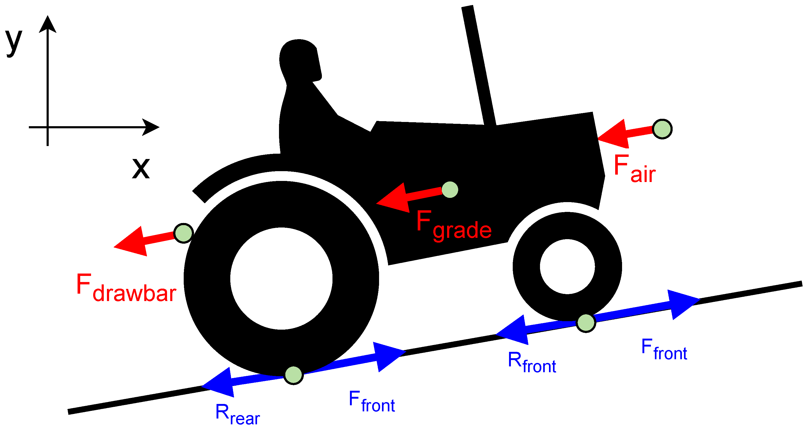
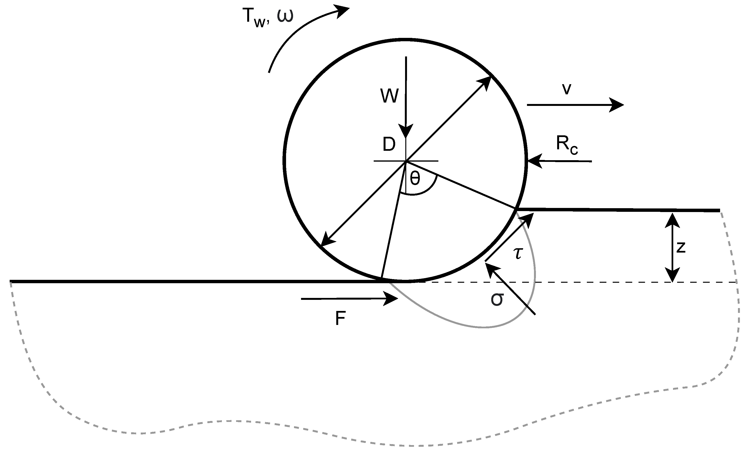
2.2. Model Development

The forces acting on a vehicle moving over an inclined terrain are shown in Figure 1. The longitudinal dynamics can be calculated according to the following force balance equation:
v ˙ = F R F a i r F g r a d e F d r a w b a r m
where F is the sum of the tractive efforts acting on the wheels, R is the sum of the motion resistances acting on the wheels, F a i r is the aerodynamic resistance, F g r a d e is the grade resistance, and F d r a w b a r is the drawbar pull.
The torque balance of the wheel dynamics is written as follows:
ω ˙ = T w T f F r J w
where ω and J w are the angular velocity and inertia of the wheel, T f is the friction, and T w is the input torque of the wheel.
First, some of the forces are neglected to simplify model development. While it significantly affects the behavior of the vehicle at higher velocities, the aerodynamic resistance below 48 km/h can be neglected [29]. Hence, it is omitted from the model. The drawbar pull is the amount of horizontal force available to a vehicle at the drawbar for pulling a load. In our case, the drawbar pull is assumed to be zero, and the remaining force accelerates the vehicle. In Figure 1, the color red notes the neglected forces, while the forces taken into account are blue. Therefore, the nonlinear state-space model describing the movement of a single wheel on a flat terrain is written as follows:
v ˙ ( t ) ω ˙ ( t ) = F R m T w T f F r J
Based on the simplified model of the wheel–soil interaction shown in Figure 2, the equilibrium of the horizontal and vertical forces is written as follows:
R c = b 0 θ 0 σ r sin θ d θ
W = b 0 θ 0 σ r cos θ d θ
where b and r are the smaller dimensions of the contact patch and radius of the wheel, and θ 0 is the contact angle of the wheel.
To predict the performance of a rigid wheel, Bekker [30] assumed that the terrain reaction on the contact patch is purely radial and is equal to the normal pressure beneath a sinkage plate:
σ r sin θ d θ = p d z
σ r cos θ d θ = p d x
where θ and z are the angle and sinkage shown in Figure 2, σ is the radial pressure on the wheel–terrain interface, and p is the normal pressure below a sinkage plate.
Combining (5) and (7), the motion resistance is written as follows:
R c = b 0 z p d z
For homogeneous soils, Bernstein [31] proposed an empirical model to describe their pressure–sinkage relationship:
p = k z n
where k is the sinkage modulus, and n is the sinkage exponent.
Later, Bekker [32] separated the sinkage modulus used by Berstein into two parts to represent both the soil cohesion and the effect of the internal shearing resistance:
p = k c b + k ϕ z n
where k c is the cohesive modulus of deformation, k ϕ is the frictional modulus of deformation, and b is the smaller dimension of the contact patch.
Substituting the pressure–sinkage Equation (11) into (9), the motion resistance is rewritten as:
R c = b t i 0 z r ( k c b + k ϕ ) z n d z
The solution of the definitive integral along the sinkage is the following:
R c = b t i k c b + k ϕ z n + 1 n + 1
For the geometry shown in Figure 2, assuming slight sinkage and expressing the sinkage from (8), the motion resistance of wheeled vehicles can be expressed in a closed form [29]. This solution takes a highly nonlinear form; thus, it is not optimal for state-space models.
According to Bekker, the thrust–slip relationship of a tire can be determined as that of a rigid track. First, the shear stress developed at the running gear–terrain interface must be calculated to calculate the tractive effort. For plastic soils, ref. [33] proposed a modification of Bekker’s equation to describe the shear stress–displacement relationship:
τ τ m a x = 1 e j K
where τ and τ m a x are the shear stress and the maximum shear stress, respectively, j is the shear displacement, and K is the shear deformation parameter.
The maximum shear displacement that the terrain can bear is defined using the Mohr–Coulomb equation:
τ m a x = c + σ tan ϕ
where c is the cohesion, σ is the normal stress below the track, and ϕ is internal angle of friction of the terrain.
The shear displacement is the relative movement between the running gear and the terrain, which causes slip. The slip can be expressed as follows:
i = 1 V r ω = 1 V V t = V t V V t = V j V t
where ω , V, V t , and V j are the rotational speed, actual forward velocity, theoretical forward speed, and slip speed of the running gear, respectively.
At a given point, which is at x distance from the front of the contact patch, the shear displacement can be written as:
j = V j t = V j x V t = i x
where t is the contact time of the point.
Then, assuming uniformly distributed normal pressure below the running gear, the equation describes the shear stress–displacement relationship:
F = b 0 l τ m a x 1 e j K d l
Calculating the definitive integral along the length of the contact patch results in the following equation:
F = A c + W tan ϕ 1 k i l 1 e i l k
where A and l are the area and length of the contact patch, while W is the normal force.
The viscous friction acting on the wheel is calculated as follows:
T f = b f ω
where b f is the viscous friction coefficient.
Substituting (13), (19), and (20) into (4), the nonlinear state-space model takes the following form:
v ˙ ( t ) ω ˙ ( t ) = A c + W tan ϕ 1 k i l 1 e i l K b t i k c b + k ϕ z n + 1 n + 1 m T w b ω A c + W tan ϕ 1 k i l 1 e i l K r J
Next, some simplifications must be made to create an LPV representation from the nonlinear model. While the exponential term e i l K could be handled as one of the scheduling parameters of the model, it rapidly converges to zero at higher slip values. For typical agricultural vehicles, such as tractors, it is negligible above 10% slip. Thus, it can be neglected under normal operational conditions. As a result, the tractive effort is formulated as follows:
F = τ m a x A 1 k i l
Furthermore, substituting Bekker’s pressure–sinkage Equation (11) into the closed form equation of the motion resistance (13) yields:
R c = b t i k c b + k ϕ p k c b + k ϕ z n + 1
As the normal pressure is the product of the normal force and the contact patch area, the equation is rewritten as:
R c = b t i k c b + k ϕ m g k c b + k ϕ A c z n + 1
Then, k c and k ϕ can be simplified from the equation of the motion resistance:
R c = b t i m g ( n + 1 ) A c z
Due to the applied simplification, the nonlinear state-space model takes the following form:
v ˙ ( t ) ω ˙ ( t ) = τ m a x A c 1 K i l b t i m g ( n + 1 ) A c z m T w b ω τ m a x A c 1 K i l r J
As the aim of this model is to support traction control algorithms, the input of the model shall be the motor torque applied at the wheel:
u = T w
Then, the remaining time-dependent variables in the state matrix A and the input matrix B can be collected in the scheduling parameter vector ρ . However, applying Jacobi linearization using the current state and input vector would yield inapt results. The traction force (22) and the motion resistance (25) are independent of both the state vector and the input vector. Eliminating them from the state-space model would result in an unusable model. On the other hand, the traction force is a linear function of the maximum shear stress, while the motion resistance is a linear function of the static sinkage. They must be handled either as states or inputs of the model.
Including them among the states of the system would require their differential equations. Therefore, handling them as uncontrollable system inputs is a more reasonable choice:
u u c = τ m a x z
In agricultural applications, the terrain is usually known; hence, the maximum shear stress of the terrain is usually known beforehand. However, the shear stress of the soil also shows a relationship with its color [34], while online estimators, such as [35], have also been developed. Hence, it can also be determined using vision-based methods. Such methods are also applicable for determining e wheel sinkage [36].
At last, the state equation of the LPV model for a single wheel can be written as follows:
v ˙ ( t ) ω ˙ ( t ) = 0 0 0 b J v ( t ) ω ( t ) + 0 1 J T w + A c K b i m g n + 1 A c K b r i A c J 0 τ m a x z
In the case of an LTI model, the state and input matrices are constants. In (29), several parameters of the state and input matrices vary over time or change based on the inputs or states of the model. These parameters are collected in the vector of scheduling parameters:
ρ = k n A c 1 i
Next, the state-space model must be augmented to describe the behavior of a vehicle with an arbitrary number of wheels. First, v ( t ) shall be the longitudinal speed of the vehicle, and each added wheel shall have its rotational speed as a new state of the model. Then, the traction forces and motion resistances must be summarized for all wheels to determine the longitudinal velocity of the vehicle:
v ˙ ( t ) ω 1 ˙ ( t ) ω 2 ˙ ( t ) ω n ˙ ( t ) = 0 0 0 0 0 b 1 J 1 0 0 0 0 b 2 J 2 0 0 0 0 b n J n v ( t ) ω 1 ( t ) ω 2 ( t ) ω n ( t ) + 0 0 0 0 1 J 1 0 0 0 0 1 J 2 0 0 0 0 0 1 J n T w 1 T w 2 T w n + A c 1 k 1 b 1 i 1 m 1 g cos α 1 n 1 + 1 A c 1 A c 2 k 2 b 2 i 2 m 2 g cos α 2 n 2 + 1 A c 2 A c n k n b n i n m n g cos α n n n + 1 A c n k 1 b 1 r 1 i 1 A c 1 J 1 0 0 0 0 0 0 0 k 2 b 2 r 2 i 2 A c 2 J 2 0 0 0 0 0 0 0 k n b n r n i n A c n J n 0 τ 1 , m a x z 1 τ 2 , m a x z 2 τ n , m a x z n
where the indices 1, 2, and n refer to the states of the corresponding wheel.

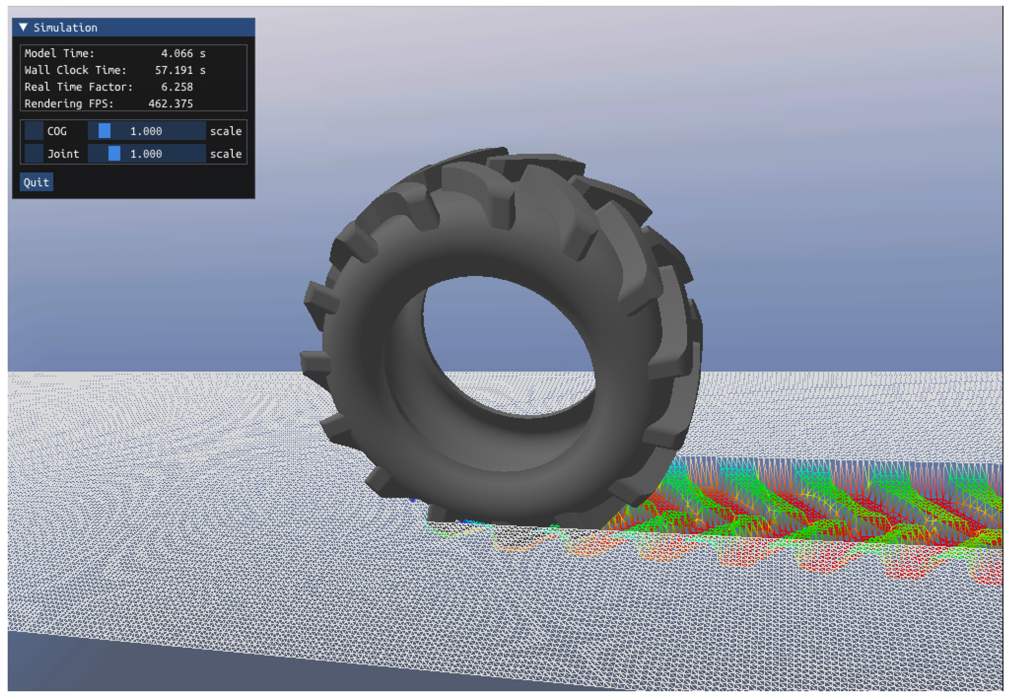
2.3. Implementation Details

The developed model was implemented using a Matlab R2023b function. There were five groups of input arguments for the function:
  • The actual state vector of the model;
  • The model parameters (such as the wheel inertia, assumed to be constant);
  • The inputs of the model over time;
  • The actual scheduling parameter vector;
  • The simulation time.
The function determines the actual inputs of the model based on the simulation time. Thus, variable step solvers can be used for simulation. Using the derived LPV model, the function determines and returns the gradient of the state vector. During simulation, a function handle was created for the function of the state-space model, whose arguments were the simulation time and the state vector. Then, the function handle was passed to the selected ordinary differential equation (ODE) solver. The results presented in this paper qwew attained using a variable-step Runge–Kutta (ODE45) method.

3. Results

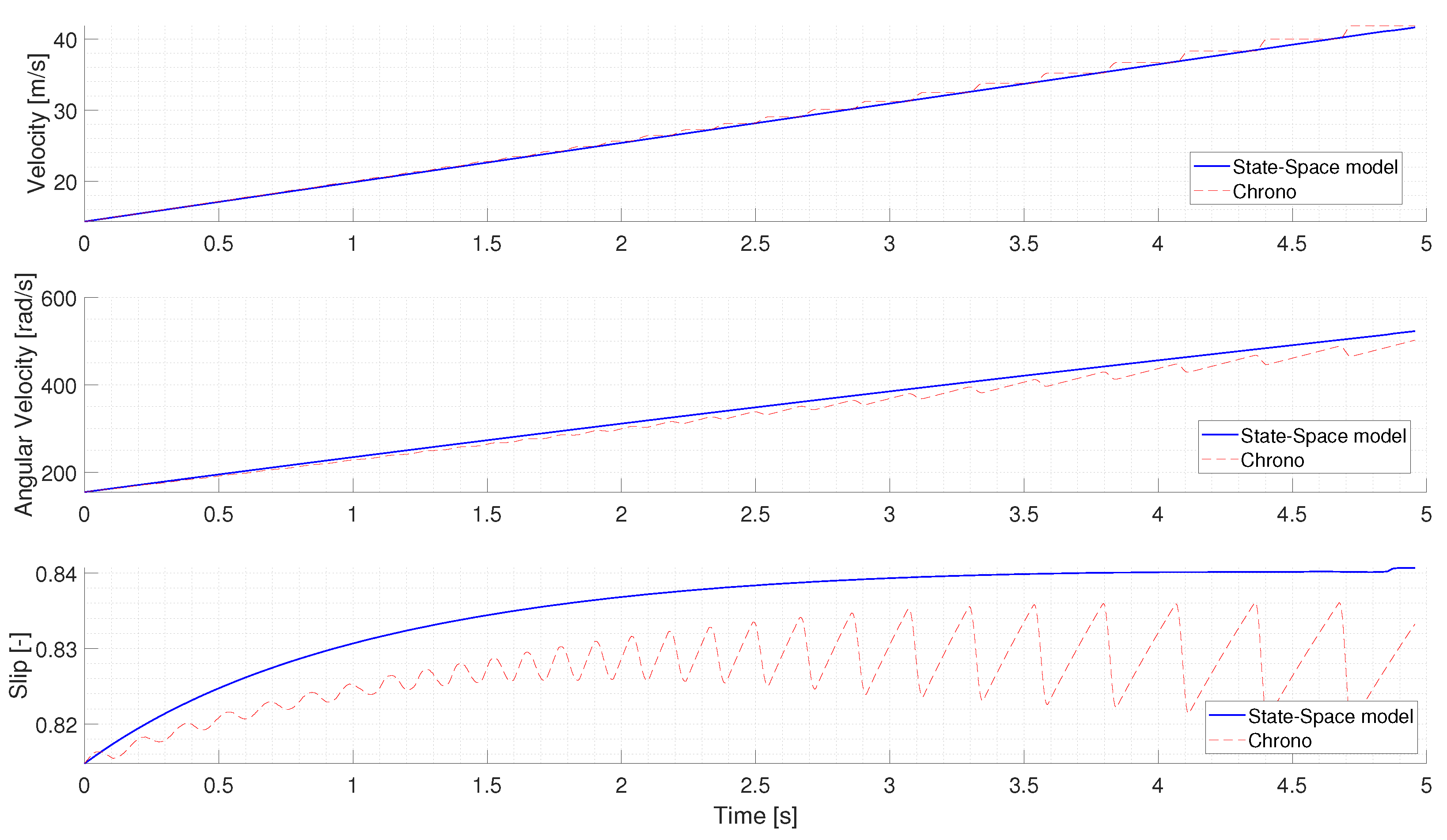
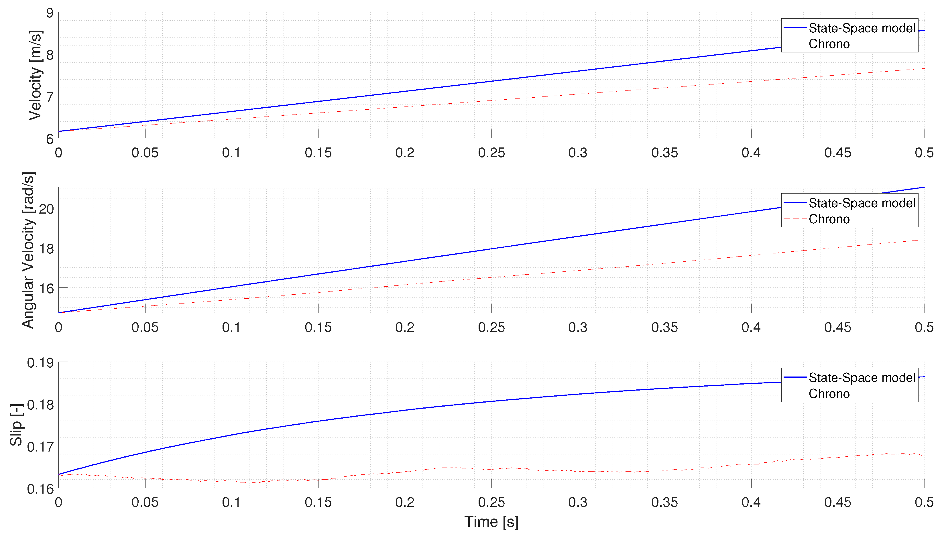
3.1. Simulation Results

First, the developed model was verified using Project Chrono [37], an open-source multiphysics simulation engine. It has various applications, such as vehicle dynamics, terramechanics, granular flows, and seismic engineering. Built upon the Bekker–Wong soil model, it is capable of modeling the operation of wheeled and tracked vehicles on deformable terrain. Custom parameters defining soil types can be assigned to every point of the managed map. The simulator features dynamic models of various wheeled and tracked vehicles with numerous suspension, drivetrain, and steering system configurations. Furthermore, custom vehicle models can also be implemented.
Project Chrono supports multi-ore, distributed computing modes and can harness GPU power for particle motion modeling. It can be faster than real time when using rigid surfaces, although its performance significantly degrades with increasing deformable terrain size. The environment created in Project Chrono is presented in Figure 3. It consisted of flat terrain created using the Soil Contact Model (SCM) deformable terrain class [38], built upon the Bekker–Wong theory, but also taking into account contact kinematics and the pressure distribution in the footprint. The terrain was modeled using a mesh, which could be deformed only in the vertical direction.
On the other hand, the LPV model was a lumped model, which also neglected the velocity of the impact on the sinkage. Hence, for the same soil type, the contact area remained constant. In Project Chrono, the wheel is created slightly above the ground to avoid unintended collision detection and numerical instabilities at the start of the simulation.
After the wheel touches the ground, a constant torque of ca. 3140 Nm is applied to the wheel, which is also used as the input of the state-space model. The comparison consisted of test cases with different terrains. For example, the parameters used to simulate a cohesionless, purely frictional terrain (LETE Sand) are summarized in Table 1.
First, the test case was simulated in Chrono, and the simulated states were exported to a text file. Then, ithey were imported to Matlab to feed the relevant inputs of the simulation to the LPV model and to perform the comparison.
The comparison of the models is presented in Figure 4. The first diagram shows the longitudinal velocity, the second diagram presents the angular velocity, and the third diagram shows the wheel slip. The slip of the LPV model envelops that of the simulator, and the quantitative results are nearly identical; the maximum difference between the calculated slips is below 2%. An increasing oscillation could also be observed in the outputs of the simulator, which was caused by the ideal motor driving the wheel and the spring-like modeling of the contact.
The tests were carried out using different wheel torques. Another example is presented in Figure 5, where the input torque is ca. 1570 Nm. As can be seen, the difference between the two models increases in the case of lower slip values. The LPV model overestimates the angular and longitudinal velocities compared to the Chrono simulation. While there is a difference between the exact values, the main characteristics of the two models are similar. Furthermore, overestimating the values errs on the side of caution.

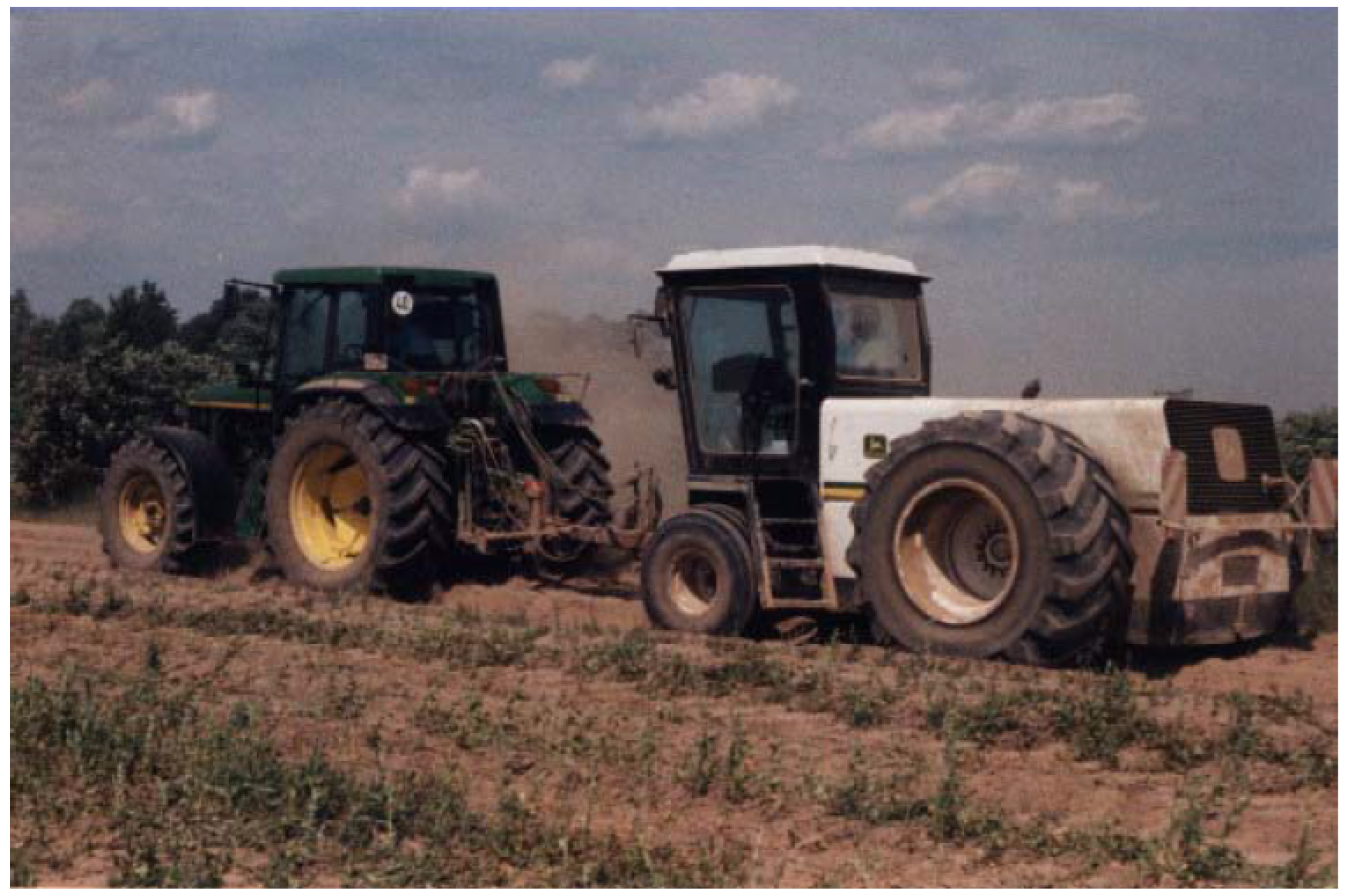
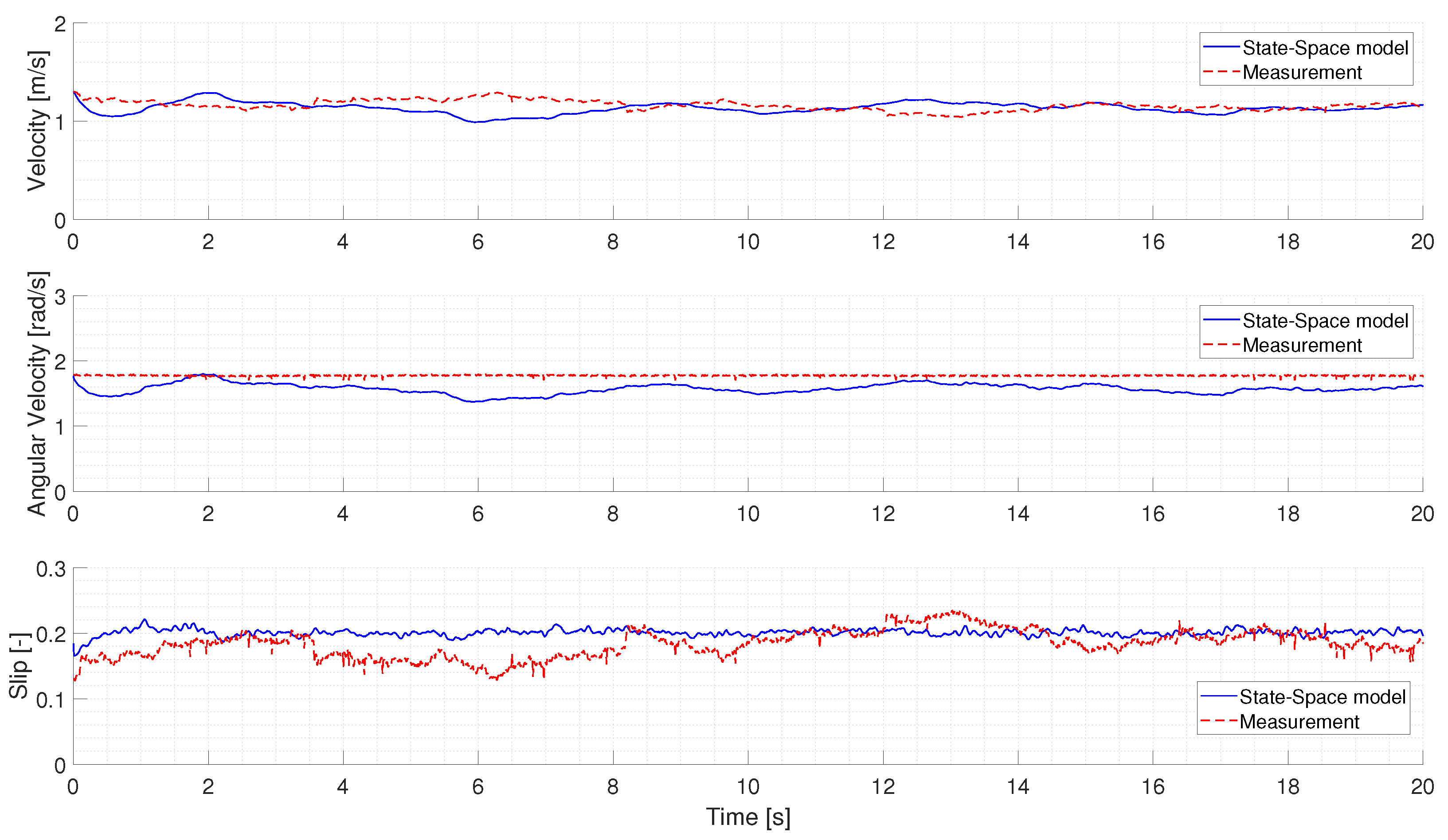
3.2. Experimental Measurements

The model was also validated against experimental measurements. The measurements used to validate the developed model were obtained previously to analyze the energetic balance of tractors. Several studies have presented results regarding the energy balance aspects, such as [39,40].
The measurements were conducted using a John Deere 6600 tractor and a Dyna-Cart dynamometer vehicle shown in Figure 6 on a flat, sandy-clay terrain. The measurements aimed to determine the energy absorption of the terrain; hence, the traction force was nearly constant during the measurements. The original drive shafts were replaced with shafts equipped with strain gauge stamps to determine the torque of the rear wheels. The measurements were conducted on straight sections, with the rear axle differential locked. Therefore, only one measurement point was sufficient to determine the rear wheel speeds, to which an electronic tachometer was used. The longitudinal velocity of the vehicle was measured using a radar.
Each measurement was conducted on virgin, undisturbed track sections to determine vertical soil deformation. The vertical terrain profile was measured in front of the tractor, in the expected wheel path, and behind the tractor, in the remaining wheel path, to determine the vertical soil deformation under the tractor wheels. Soil samples were taken from various parts of the field, and their composition, density, volume weight, water content, and porosity were determined in a laboratory to determine the soil properties of the experimental area. However, the Bekker–Wong terrain parameters of the soil were not determined during the measurement presented in [29,34] for similar types of soils with the same moisture content. The same applies to the inertia of the wheel: the vehicle mass is, in this case, half of the mass on the rear axle of the tractor, which was measured using a weight-bridge. The parameters used for validation are summarized in Table 2.
Figure 7 presents the validation results. As in the case of the verification results, the first diagram shows the longitudinal velocity, the second diagram presents the angular velocity, and the third diagram shows the wheel slip. During the measurements, the total fraction force was nearly constant, although there was a slight oscillation in the torque measured at the wheels, which was used as the input of the model. The oscillation of the torque resulted in a similar behavior in the simulated angular velocity, although it was nearly constant during the measurements, which indicated that the reduced inertia of the wheel and the transmission system was underestimated.
The absolute differences between the simulated and measured velocities are small. The maximum absolute error of the longitudinal velocity is below 0.3 m/s and 0.5 rad/s in the case of the angular velocity. On the other hand, the relative errors are significant due to the low reference values, which is also reflected in the slip, where the absolute error of the model reaches 0.06. While the difference could be caused by both parameter uncertainty and simplifications of the model, it is interesting to note that the errors significantly decrease after 8 seconds.

4. Discussion

The deviation of the LPV model compared to both the Chrono simulators and the experimental measurements are summarized in Table 3. Quantitatively, the most significant deviance can be seen in the case of the angular velocity error during the high-slip simulation, which comes from the sawtooth-like form of the angular velocity simulated in Chrono. The absolute differences are low in all other cases.
According on the results, the proposed model can describe the behavior of off-road vehicles with an accuracy acceptable for control design. Furthermore, it can run in real-time: the simulation of 10 s of driving required approximately 0.0365 s. Yet, the proposed model has some drawbacks, which must be discussed. Due to the applied simplifications, the operating domain of the model was narrowed. As Figure 5 shows, the accuracy of the model decreases in the case of lower slip values, which is caused by neglecting the exponential term in (19). Similarly, its performance degrades in the presence of a significant slope or if the velocity of the vehicle increases.
On the contrary, grid-based LPV models often suffer from the curse of dimensionality. Narrowing the operation domain of the model reduces the number of grid points, simplifying control synthesis. Depending on the requirements of the control design, it is possible to include the neglected forces in the LPV model.
Some model parameters, such as the area of the contact patch or the terrain parameters, are difficult to measure or estimate in real time. Even if the terrain is traversed in advance, the accuracy of these parameters is uncertain, or they could have changed since the measurement. While this is a common drawback of semiempirical models, robust control techniques, such as the LPV H algorithm, can handle parameter uncertainty.
On the other hand, the number of terrain parameters was reduced compared to the original equations, and grid-based LPV models can provide some robustness against measurement errors in the scheduling parameters. Furthermore, contrary to several of the adapted on-road tire models, the proposed model takes into account the characteristics of the vehicle; hence, the same model can be used for different vehicles without any intermediate steps, contrary to the adapted on-road models.

5. Conclusions

An LPV model was developed for off-road vehicles, which aims to model terrain–vehicle interactions in real time with acceptable accuracy and support the development of model-based control algorithms. First, a nonlinear state-space model was derived from the Bekker–Wong equations; then, it was simplified and reformulated using the LPV approach.
Next, the model was verified using Project Chrono, a multiphysics simulator, and validated against experimental measurements. Based on the results, the accuracy of the developed model is suitable for control design purposes. Furthermore, off-road traction control algorithms have to estimate the terrain parameters, which can be computationally expensive and inaccurate. The proposed model requires only three terrain parameters: the shear deformation coefficient, the sinkage exponent, and the maximum shear stress. Thus, the uncertainty caused by the accuracy of the estimated parameters can be reduced.
The proposed model can be used to design model-based estimator algorithms, such as different variants of the Kalman filter algorithm. However, in this case, the uncontrollable and controllable inputs can be combined into a single input vector to simplify the design process.
Traction control algorithms usually aim to control either the slip or the longitudinal velocity of the vehicle. However, in the presented form of the model, the latter is an uncontrollable state as it is independent of the controllable input and the controllable states of the model. It depends only on the uncontrollable inputs of the system. A possible solution is using the slip or its reciprocal as a system state instead of a scheduling parameter. This way, both the slip and the longitudinal velocity become controllable states of the system. The nonlinearities caused by the inclusion of the slip among the state variables can also be handled by the LPV representation. LPV-based slip ratio controllers are already presented in the literature for on-road vehicles, such as the method presented in [41].
Further work will focus on the generalization of the presented model and the improvement in the model’s accuracy. The possibility of considering the effects of steep slopes, different pressure–sinkage values, shear stress–displacement models, or even organic terrain must be analyzed.

Author Contributions

Conceptualization, A.S. and P.K.; methodology, A.S. and P.K.; software, D.K.D.; validation, P.K. and D.K.D.; writing—original draft preparation, A.S. and D.K.D.; writing—review and editing, S.A.; visualization, S.A.; supervision, S.A. All authors have read and agreed to the published version of the manuscript.

Funding

This research was supported by the Ministry of Culture and Innovation and the National Research, Development and Innovation Office within the Cooperative Technologies National Laboratory of Hungary (grant No. 2022-2.1.1-NL-2022-00012).

Data Availability Statement

The data presented in this study are available upon request from the corresponding author.

Conflicts of Interest

The authors declare no conflicts of interest.

Abbreviations

The following abbreviations are used in this manuscript:
ABSAntilock Braking System
ACCAdaptive Cruise Control
DASDriver Assistance System
DEMDiscrete Element Method
FEMFinite Element Method
LFRLinear Fractional Representation
LFTLinear Fractional Transformation
LPVLinear Parameter-Varying
qLPVQuasi-Linear Parameter-Varying
SCMSoil Contact Model

References

  1. Sunusi, I.I.; Zhou, J.; Wang, Z.Z.; Sun, C.; Ibrahim, I.E.; Opiyo, S.; Soomro, S.A.; Korohou, T.; Soomro, S.A.; Olanrewaju, T. Intelligent tractors: Review of online traction control process. Comput. Electron. Agric. 2020, 170, 105176. [Google Scholar] [CrossRef]
  2. Luo, Z.; Wang, J.; Wu, J.; Zhang, S.; Chen, Z.; Xie, B. Research on a Hydraulic Cylinder Pressure Control Method for Efficient Traction Operation in Electro-Hydraulic Hitch System of Electric Tractors. Agriculture 2023, 13, 1555. [Google Scholar] [CrossRef]
  3. Stentz, A.; Dima, C.; Wellington, C.; Herman, H.; Stager, D. A system for semi-autonomous tractor operations. Auton. Robot. 2002, 13, 87–104. [Google Scholar] [CrossRef]
  4. Upadhyaya, S.; Wulfsohn, D. Traction prediction using soil parameters obtained with an instrumented analog device. J. Terramech. 1993, 30, 85–100. [Google Scholar] [CrossRef]
  5. Rubinstein, D.; Shmulevich, I.; Frenckel, N. Use of explicit finite-element formulation to predict the rolling radius and slip of an agricultural tire during travel over loose soil. J. Terramech. 2018, 80, 1–9. [Google Scholar] [CrossRef]
  6. Jiang, M.; Dai, Y.; Cui, L.; Xi, B. Experimental and DEM analyses on wheel-soil interaction. J. Terramech. 2018, 76, 15–28. [Google Scholar] [CrossRef]
  7. Wong, J.Y.; Reece, A. Prediction of rigid wheel performance based on the analysis of soil-wheel stresses part I. Performance of driven rigid wheels. J. Terramech. 1967, 4, 81–98. [Google Scholar] [CrossRef]
  8. He, R.; Sandu, C.; Khan, A.K.; Guthrie, A.G.; Els, P.S.; Hamersma, H.A. Review of terramechanics models and their applicability to real-time applications. J. Terramech. 2019, 81, 3–22. [Google Scholar] [CrossRef]
  9. Johnson, D.K.; Botha, T.R.; Els, P.S. Real-time side-slip angle measurements using digital image correlation. J. Terramech. 2019, 81, 35–42. [Google Scholar] [CrossRef]
  10. Linström, B.V.; Els, P.S.; Botha, T. A real-time non-linear vehicle preview model. Int. J. Heavy Veh. Syst. 2018, 25, 1–22. [Google Scholar] [CrossRef]
  11. Sandu, C.; Kolansky, J.; Botha, T.; Els, S. 6.3. Multibody Dynamics Techniques for Real-Time Parameter Estimation. Adv. Auton. Veh. Des. Sev. Environ. 2015, 44, 221. [Google Scholar]
  12. Vieira, D.; Orjuela, R.; Spisser, M.; Basset, M. An adapted Burckhardt tire model for off-road vehicle applications. J. Terramech. 2022, 104, 15–24. [Google Scholar] [CrossRef]
  13. Lenain, R.; Thuilot, B.; Cariou, C.; Martinet, P. High accuracy path tracking for vehicles in presence of sliding: Application to farm vehicle automatic guidance for agricultural tasks. Auton. Robot. 2006, 21, 79–97. [Google Scholar] [CrossRef]
  14. Cariou, C.; Lenain, R.; Thuilot, B.; Berducat, M. Automatic guidance of a four-wheel-steering mobile robot for accurate field operations. J. Field Robot. 2009, 26, 504–518. [Google Scholar] [CrossRef]
  15. Kim, J.; Lee, J. Traction-energy balancing adaptive control with slip optimization for wheeled robots on rough terrain. Cogn. Syst. Res. 2018, 49, 142–156. [Google Scholar] [CrossRef]
  16. Salama, M.A.; Vantsevich, V.V.; Way, T.R.; Gorsich, D.J. UGV with a distributed electric driveline: Controlling for maximum slip energy efficiency on stochastic terrain. J. Terramech. 2018, 79, 41–57. [Google Scholar] [CrossRef]
  17. Pacejka, H.B.; Besselink, I.J.M. Magic Formula Tyre Model with Transient Properties. Veh. Syst. Dyn. 1997, 27, 234–249. [Google Scholar] [CrossRef]
  18. Alexander, A.; Sciancalepore, A.; Vacca, A. Online Controller Setpoint Optimization for Traction Control Systems Applied to Construction Machinery. In Proceedings of the BATH/ASME 2018 Symposium on Fluid Power and Motion Control, Bath, UK, 12–14 September 2018; p. V001T01A068. [Google Scholar] [CrossRef]
  19. Saunders, A.; White, D.; Compere, M. Estimating Pacejka (PAC2002) Tire Coefficients for Pneumatic Tires on Soft Soils With Application to BAJA SAE Vehicles. In Proceedings of the ASME 2019 International Mechanical Engineering Congress and Exposition, Salt Lake City, UT, USA, 11–14 November 2019; Volume 59414, p. V004T05A081. [Google Scholar]
  20. Vieira, D.; Orjuela, R.; Spisser, M.; Basset, M. Longitudinal Vehicle Control based on Off-road Tire Model for Soft Soil Applications. IFAC-PapersOnLine 2021, 54, 304–309. [Google Scholar] [CrossRef]
  21. Gaspar, P.; Szaszi, I.; Bokor, J. Active Suspension Design using LPV Control. IFAC Proc. Vol. 2004, 37, 565–570. [Google Scholar] [CrossRef]
  22. Poussot-Vassal, C.; Sename, O.; Dugard, L.; Gáspár, P.; Szabó, Z.; Bokor, J. A new semi-active suspension control strategy through LPV technique. Control Eng. Pract. 2008, 16, 1519–1534. [Google Scholar] [CrossRef]
  23. Németh, B. Robust LPV design with neural network for the steering control of autonomous vehicles. In Proceedings of the 2019 18th European Control Conference (ECC), Naples, Italy, 25–28 June 2019; pp. 4134–4139. [Google Scholar]
  24. Németh, B.; Gáspár, P.; Orjuela, R.; Basset, M. LPV-based Control Design of an Adaptive Cruise Control System for Road Vehicles. IFAC-PapersOnLine 2015, 48, 62–67. [Google Scholar] [CrossRef]
  25. Vu, V.T.; Sename, O.; Dugard, L.; Gaspar, P. The Design of an H∞/LPV Active Braking Control to Improve Vehicle Roll Stability. IFAC-PapersOnLine 2019, 52, 54–59. [Google Scholar] [CrossRef]
  26. Gáspár, P.; Németh, B.; Bokor, J. Design of an LPV-based integrated control for driver assistance systems. IFAC Proc. Vol. 2012, 45, 511–516. [Google Scholar] [CrossRef]
  27. Gáspár, P.; Szabó, Z.; Bokor, J. LPV design of adaptive integrated control for road vehicles. IFAC Proc. Vol. 2011, 44, 662–667. [Google Scholar] [CrossRef]
  28. Li, J.; Sun, S.; Sun, C.; Liu, C.; Tang, W.; Wang, H. Analysis of Effect of Grouser Height on Tractive Performance of Tracked Vehicle under Different Moisture Contents in Paddy Soil. Agriculture 2022, 12, 1581. [Google Scholar] [CrossRef]
  29. Wong, J.Y. Terramechanics and Off-Road Vehicle Engineering: Terrain Behaviour, Off-Road Vehicle Performance and Design; Butterworth-Heinemann: Oxford, UK, 2009. [Google Scholar]
  30. Bekker, M.G. Theory of Land Locomotion; University of Michigan Press: Ann Arbor, MI, USA, 1956. [Google Scholar]
  31. Bernstein, R. Probleme zur experimentellen Motorpflugmechanik. Der Mot. 1913, 16, 199–206. [Google Scholar]
  32. Bekker, M.G. Introduction to Terrain-Vehicle Systems. Part I: The Terrain. Part II: The Vehicle; University of Michigan Press: Ann Arbor, MI, USA, 1969. [Google Scholar]
  33. Janosi, Z. The Analytical Determination of Drawbar Pull as A Function of Slip for Tracked Vehicles in Deformable Soils. In Proceedings of the International Society for Terrain-Vehicle Systems, The 1st International Conference, Turin, Italy, 1961; Volume 707. [Google Scholar]
  34. El Hariri, A.; Ahmed, A.E.E.; Kiss, P. Sandy Loam Soil Shear Strength Parameters and Its Colour. Appl. Sci. 2023, 13, 3847. [Google Scholar] [CrossRef]
  35. Iagnemma, K.; Shibly, H.; Dubowsky, S. On-line terrain parameter estimation for planetary rovers. In Proceedings of the 2002 IEEE International Conference on Robotics and Automation (Cat. No. 02CH37292), Washington, DC, USA, 11–15 May 2002; Volume 3, pp. 3142–3147. [Google Scholar]
  36. Iagnemma, K.; Kang, S.; Brooks, C.; Dubowsky, S. Multi-sensor terrain estimation for planetary rovers. In Proceedings of the 8th International Symposium on Artificial Intelligence, Robotics, and Automation in Space, Nara, Japan, 19–23 May 2003. [Google Scholar]
  37. Tasora, A.; Serban, R.; Mazhar, H.; Pazouki, A.; Melanz, D.; Fleischmann, J.; Taylor, M.; Sugiyama, H.; Negrut, D. Chrono: An Open Source Multi-Physics Dynamics Engine; Springer: Berlin/Heidelberg, Germany, 2016; pp. 19–49. [Google Scholar]
  38. Krenn, R.; Hirzinger, G. SCM–A soil contact model for multi-body system simulations. In Proceedings of the 11th European Regional Conference of the International Society for Terrain-Vehicle Systems, Bremen, Germany, 5–8 October 2009. [Google Scholar]
  39. Kiss, P.; Laib, L. Tractor energy balance under instationary conditions: 6th Mini Conference on Vehicle System Dynamics, Identification and Anomalies (VSDIA’98). In Proceedings of the 6th Mini Conference on Vehicle System Dynamics, Identification and Anomalies, VSDIA’98, Budapest, Hungary, 9–11 November 1998; pp. 407–414. [Google Scholar]
  40. Kiss, P. Effect of Soil Deformation on the Energy Balance of Tractors. Hung. Agric. Eng. 1999, 12, 35–39. [Google Scholar]
  41. Jia, F.; Liu, Z. A LPV traction control approach for independent in-wheel electric motor vehicle. In Proceedings of the 11th World Congress on Intelligent Control and Automation, Shenyang, China, 29 June–4 July 2014; pp. 1992–1997. [Google Scholar] [CrossRef]
Figure 1. Forces acting on an off-road vehicle.
Agriculture 14 00499 g001
Figure 2. Rigid wheel–deformable terrain interaction.
Agriculture 14 00499 g002
Figure 3. Project Chrono simulation environment.
Agriculture 14 00499 g003
Figure 4. Verification of the proposed LPV model using Project Chrono—high slip.
Agriculture 14 00499 g004
Figure 5. Verification of the proposed LPV model using Project Chrono—low slip.
Agriculture 14 00499 g005
Figure 6. John Deere 6600 tractor and Dyna-Cart dynamometer vehicle.
Agriculture 14 00499 g006
Figure 7. Validation of the proposed LPV model.
Agriculture 14 00499 g007
Table 1. Terrain and vehicle parameters—Project Chrono simulation.
Terrain parametersSinkage coefficient [-]1.1
Cohesion [Pa]0
Shear deformation modulus [m]0.01
Friction angle [°]30
Contact area [m2]0.224
Vehicle parametersWheel inertia [kgm2]20
Vehicle mass [kg]500
Wheel width [m]0.4
Wheel radius [m]0.5
Table 2. Terrain and vehicle parameters—measurement.
Terrain parametersSinkage coefficient [-]0.85
Cohesion [Pa]2200
Shear deformation modulus [m]0.08
Friction angle [°]30
Contact area [m2]0.224
Vehicle parametersWheel inertia [kgm2]20
Vehicle mass [kg]1662.5
Wheel width [m]0.46
Wheel radius [m]0.9
Table 3. Performance metrics of the LPV model.
High-Slip SimulationLow-Slip SimulationMeasurement
Velocity [m/s]Max1.4060.9080.283
Mean0.3140.4560.075
Angular velocity [rad/s]Max40.6312.6500.423
Mean14.7061.4160.202
Slip [-]Max0.020.0190.076
Mean0.0080.0150.022
Disclaimer/Publisher’s Note: The statements, opinions and data contained in all publications are solely those of the individual author(s) and contributor(s) and not of MDPI and/or the editor(s). MDPI and/or the editor(s) disclaim responsibility for any injury to people or property resulting from any ideas, methods, instructions or products referred to in the content.

