Non-Contact Measurement of Pregnant Sows’ Backfat Thickness Based on a Hybrid CNN-ViT Model

Abstract

Backfat thickness (BF) is closely related to the service life and reproductive performance of sows. The dynamic monitoring of sows’ BF is a critical part of the production process in large-scale pig farms. This study proposed the application of a hybrid CNN-ViT (Vision Transformer, ViT) model for measuring sows’ BF to address the problems of high measurement intensity caused by the traditional contact measurement of sows’ BF and the low efficiency of existing non-contact models for measuring sows’ BF. The CNN-ViT introduced depth-separable convolution and lightweight self-attention, mainly consisting of a Pre-local Unit (PLU), a Lightweight ViT (LViT) and an Inverted Residual Unit (IRU). This model could extract local and global features of images, making it more suitable for small datasets. The model was tested on 106 pregnant sows with seven randomly divided datasets. The results showed that the CNN-ViT had a Mean Absolute Error (MAE) of 0.83 mm, a Root Mean Square Error (RMSE) of 1.05 mm, a Mean Absolute Percentage Error (MAPE) of 4.87% and a coefficient of determination (R-Square, R²) of 0.74. Compared to LviT-IRU, PLU-IRU and PLU-LviT, the CNN-ViT’s MAE decreased by more than 12%, RMSE decreased by more than 15%, MAPE decreased by more than 15% and R² improved by more than 17%. Compared to the Resnet50 and ViT, the CNN-ViT’s MAE decreased by more than 7%, RMSE decreased by more than 13%, MAPE decreased by more than 7% and R² improved by more than 15%. The method could better meet the demand for the non-contact automatic measurement of pregnant sows’ BF in actual production and provide technical support for the intelligent management of pregnant sows.

1. Introduction

The reproductive performance of the sow is one of the most important indicators of economic efficiency in pig production. Backfat is laminar adipose tissue located subcutaneously on the sow’s back. It can provide energy for its daily activities and excretes a large number of active substances, which is significantly correlated with its health [1] and reproductive performance [2]. Backfat thickness (BF) can affect the placental function of the sow. BF that is either too thick or too thin can increase the chance of placental inflammation, which affects the sow’s litter size [3,4]. BF also affects the sow’s service life [5,6]. Sows with thicker BF tend to reach puberty early and have a lower elimination ratio [7]. However, BF that is too thin is also not helpful in extending the life span of the sow. In addition, BF at different gestation periods also affects the sow’s reproductive performance [8]. The sow’s reproductive performance is best when its BF is maintained at 18~20 mm in early gestation, ≥20 mm in mid-gestation and 14~16 mm in late gestation [9]. Different gestation periods have different requirements for sows’ BF, which is often used in production to divide the feeding stages. Therefore, dynamic monitoring of sows’ BF is critical to improving sow reproductive performance and pig productivity.

Currently, visual pressure, ultrasonic measurement [10] and CT scan [11] are the three main methods used to measure the BF of pigs in production. They are labor intensive, inefficient and difficult to meet the needs of pig farms for the automatic measurement of sows’ BF, which affects the production efficiency. With the continuous development of image processing technology and deep learning [12], the non-contact estimation method of the livestock body condition has become a new research direction in livestock phenomics. Teng et al. [13] extracted the radius of curvature of the sow’s hip from its point cloud data and found a correlation between this feature and BF, indicating that the non-contact measurement of BF could be accomplished by hip images. Compared with the rear view acquisition of sow hip images, the top view is easier to standardize and automate. The image of the pig’s back in the top view includes different parts of the pig such as the shoulder, the last costal bone and the hip, where the BF measurements correlate with the actual carcass fat thickness. Fernandes et al. [14] used 3D back images of finishing pigs from a top view to construct a CNN model to measure BF. A comparison of the measurement accuracy with manually defined features and CNN automatically extracted features showed that the deep learning method could achieve higher accuracy. Point cloud data or a depth map can be used to acquire more dimensional information, but their accuracy will be affected by the environment with limited scenarios and higher costs [15,16]. Yu et al. [17] constructed a CNN-BGR-SVR model to measure the BF of pregnant sows based on 2D images of the sows’ backs and used BGR features that took into account the heritability of BF. The study showed that the BF could be non-contact measured using 2D back images. However, this method required the continuous measurement of BF over a certain period, which is inefficient. Research on the measurement of pigs’ BF based on computer vision is just beginning, but there is more research on the non-contact body condition estimation of cows. Alvarez et al. [18] constructed an end-to-end CNN to directly estimate the body condition from the depth of the cow’s back, contour edges and Its Fourier-transformed images, overcoming the limitations of manually defined features. To further enhance the feature extraction ability of the model, the addition of attention to the model when estimating the body condition of cows has become a new research direction [19,20]. Shi et al. [21] showed that the addition of attention could improve the estimation accuracy of the cow body condition model. The existing method of non-contact measurement of pregnant sows’ BF based on 2D images was complicated and mainly used CNN structures to extract local features of images, with an inadequate global feature extraction ability [22]. Different regions in a sow’s back image contribute differently to the prediction of its BF. The traditional CNN structure is limited in its ability to focus on the key information in the image [23], which limits the accuracy and generalization ability of the model.

Vision Transformer (ViT), which is based on self-attention, can capture long-distance dependencies in images and extract global features of images, and it is becoming a new direction in the field of computer vision [24]. ViT has been applied in various fields including industry [25], medicine [26] and agriculture [27] but currently has fewer applications in the field of livestock phenotypic measurements. The outstanding performance of ViT is based on a huge data size and sacrifices a large number of computational resources, making it difficult to apply to small datasets [28]. By contrast, CNN performs more consistently on different types of tasks [29], and it has been widely used in various fields [30,31]. Therefore, this study focuses on the need for the non-contact automatic measurement of pregnant sows’ BF and addresses the problems of the low efficiency of existing methods and the insufficient global feature extraction ability of the CNN structure. This study introduced a ViT structure with self-attention as the core and constructed an efficient automatic measurement model of pregnant sows’ BF based on CNN-ViT. This model combined the local and global features of the images, allowing the measurement of sows’ BF with a small dataset and computational resources. The aim of this study was to provide an efficient method for the non-contact measurement of pregnant sows’ BF. The study outcomes highlighted in Figure 1 show the CNN-ViT methodology flowchart applied to non-contact measurements of pregnant sows’ BF.

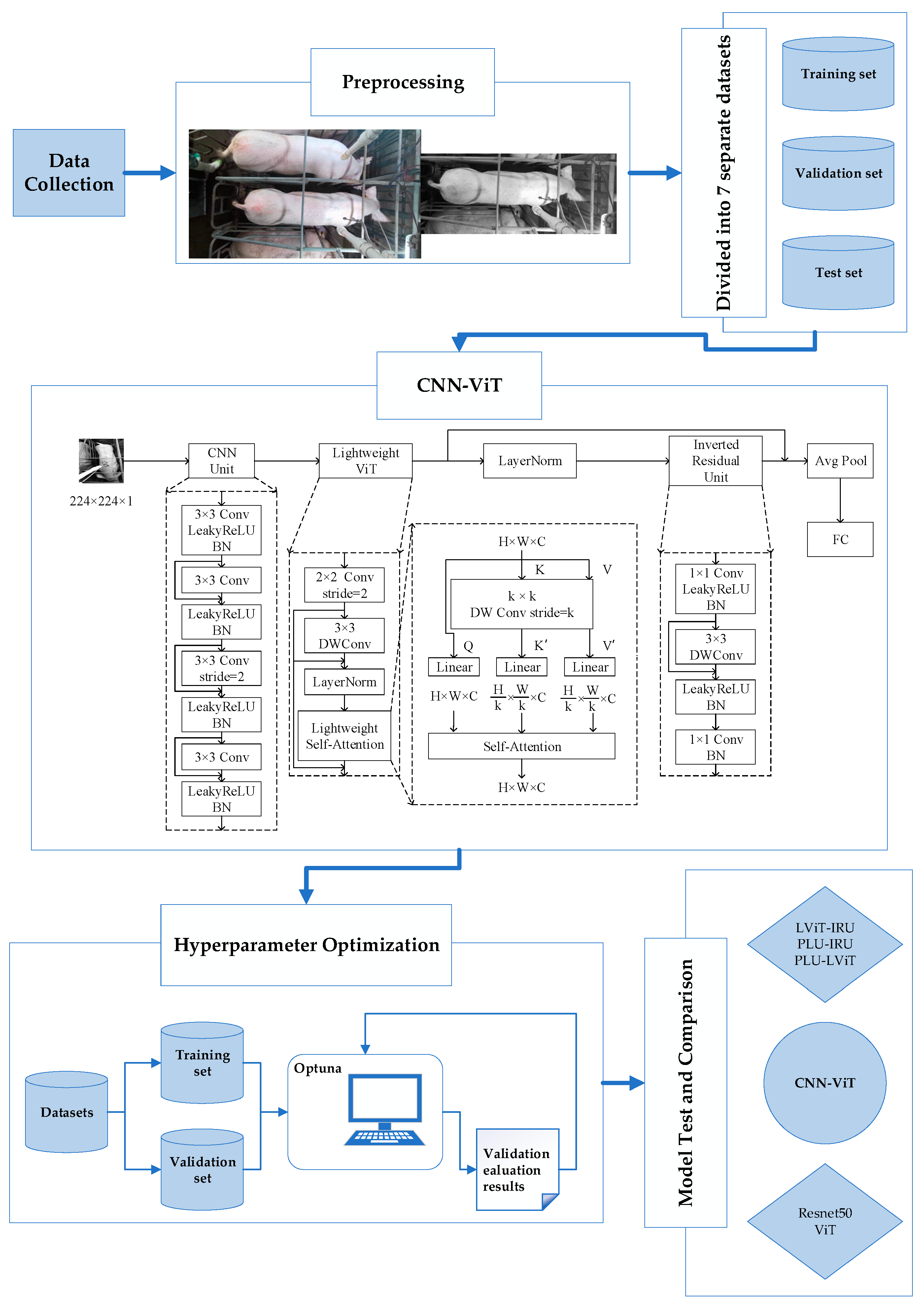
2. Materials and Methods

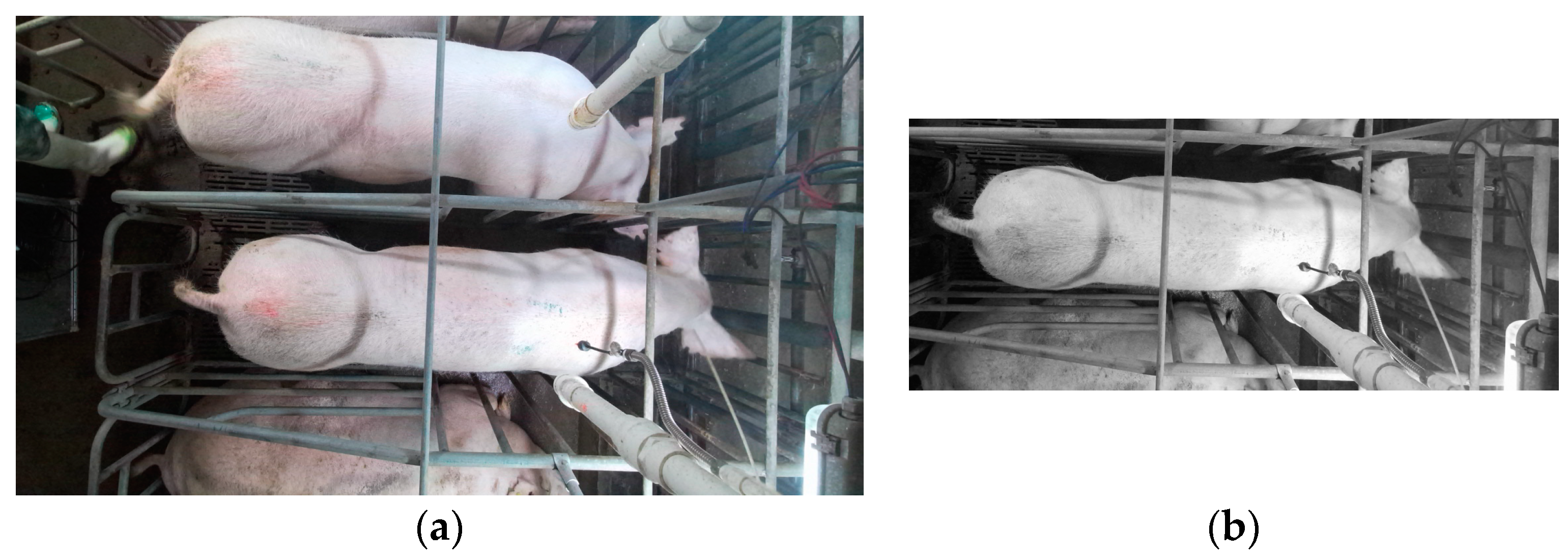
2.1. Data Collection

The data were collected in July and August 2021 at a sow farm. A total of 106 pregnant sows were collected, including 58 sows in the early gestation and 48 sows in mid-gestation. Sows were fed in single pens, with sows in different gestation periods fed in different buildings. An Azure Kinect camera was set up on a self-built adjustable mobile trolley to record video data of the sow’s back while standing in a top–down view. The camera recorded video at 30 frames per second, and 3 min of video was recorded for each sample. Sows’ BF was measured with a Renco (LEAN-METER) backfat meter; the measuring point was the P2 commonly used in the international pig industry [32].

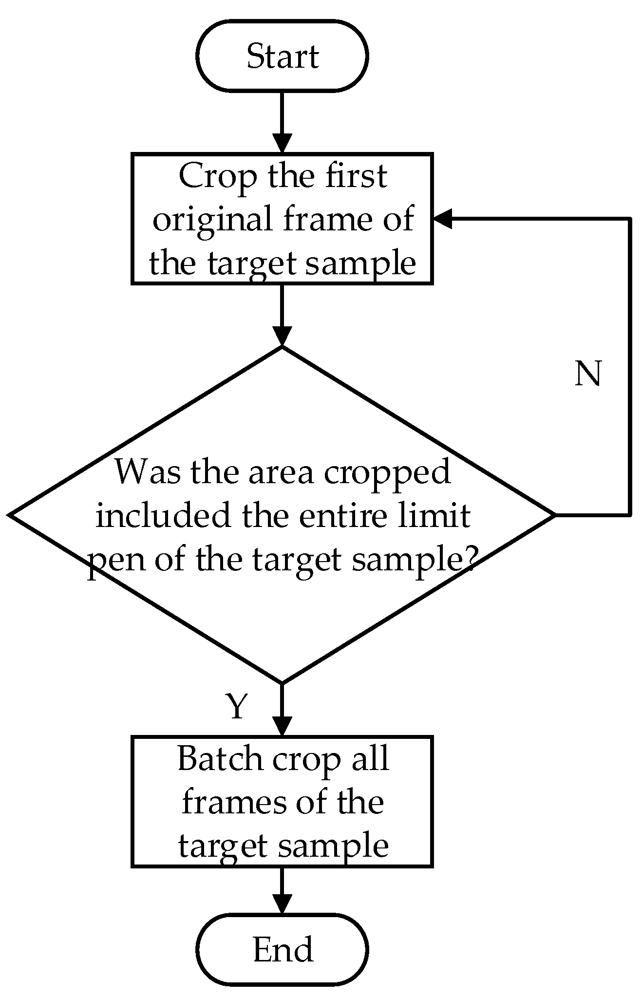
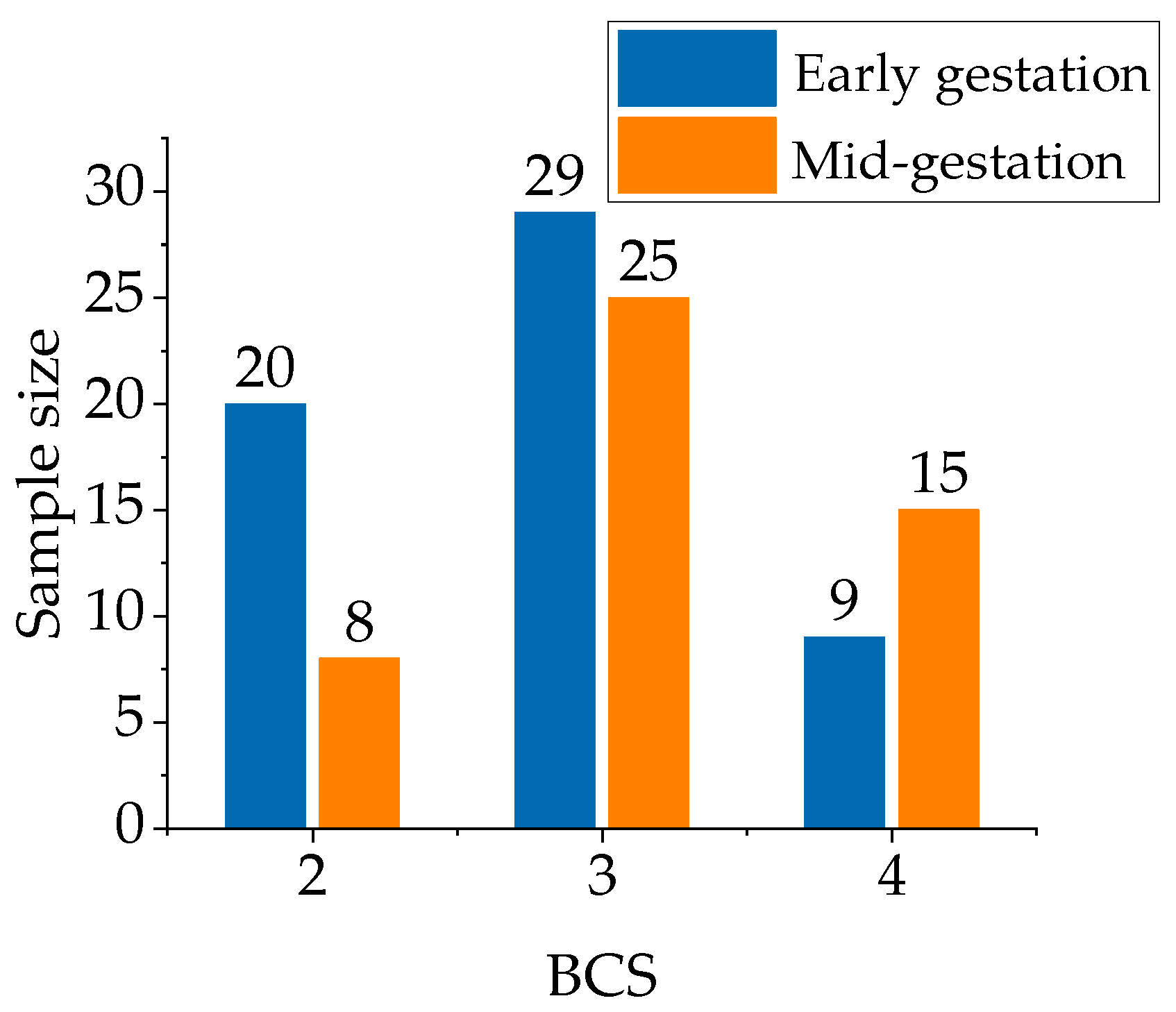
2.2. Dataset Production

The recorded video of each sample was parsed into RGB images. To ensure the differences between data, one frame of video was captured every 2 s. A total of 90 images per sample were captured, with 9540 images constituting the sows’ BF measurement image dataset. The single RGB image was noisy due to its 1280 × 720 pixels containing samples of sows from other pens. To minimize the effect of extra sows and ensure the integrity of the required sample of sows, every image was cropped. The limit pen was selected as the target area for cropping; the size of the cropped area was fixed at 1080 × 450. The flow of cropping images is shown in Figure 2.

The cropped images still contained a lot of noisy information, including the back-ground and color. As the sows’ BF is mainly related to its body size, the sow’s skin color was not a useful predictor of its BF. Therefore, all cropped images were grayed to im-prove the model computation speed and modeling efficiency. A comparison of the data before and after pre-processing is shown in Figure 3.

According to the body condition score (BCS) of pigs shown in

Table 1. Chart of sows’ body condition score.

BCS	BF/mm
1	<10
2	≥10~15
3	>15~18
4	>18~22
5	>22

, the BF of the samples collected in this study were within the range of 2, 3 and 4. As shown in Figure 4, the number of sows collected in the early and mid-gestation was approximately the same. However, the distribution of gestation within different BCSs was different. A higher percentage of sows in the early gestation was found with a BCS of 2 and 3, and a higher percentage of sows in the mid-gestation was found with a BCS of 4. To ensure the adequacy of training samples, as well as the uniformity and consistency of the sample distribution in each dataset, the dataset was randomly divided into a training set, validation set and test set according to the gestation periods and sow BCS by 8:1:1. The distribution of samples in each dataset is shown in

Table 2. Dataset division.

Dataset	Gestation	BCS			Total
		2	3	4
Train	Early	16	23	8	86
	Mid	7	20	12
Validation	Early	2	3	1	10
	Mid	1	2	1
Test	Early	2	3	0	10
	Mid	0	3	2

. In order to adequately verify the generalization ability of the model on different samples and reduce the bias in the performance estimates, multiple datasets were divided [33,34]. According to Table 2, 7 different datasets were divided and a total of 70 different samples were tested.

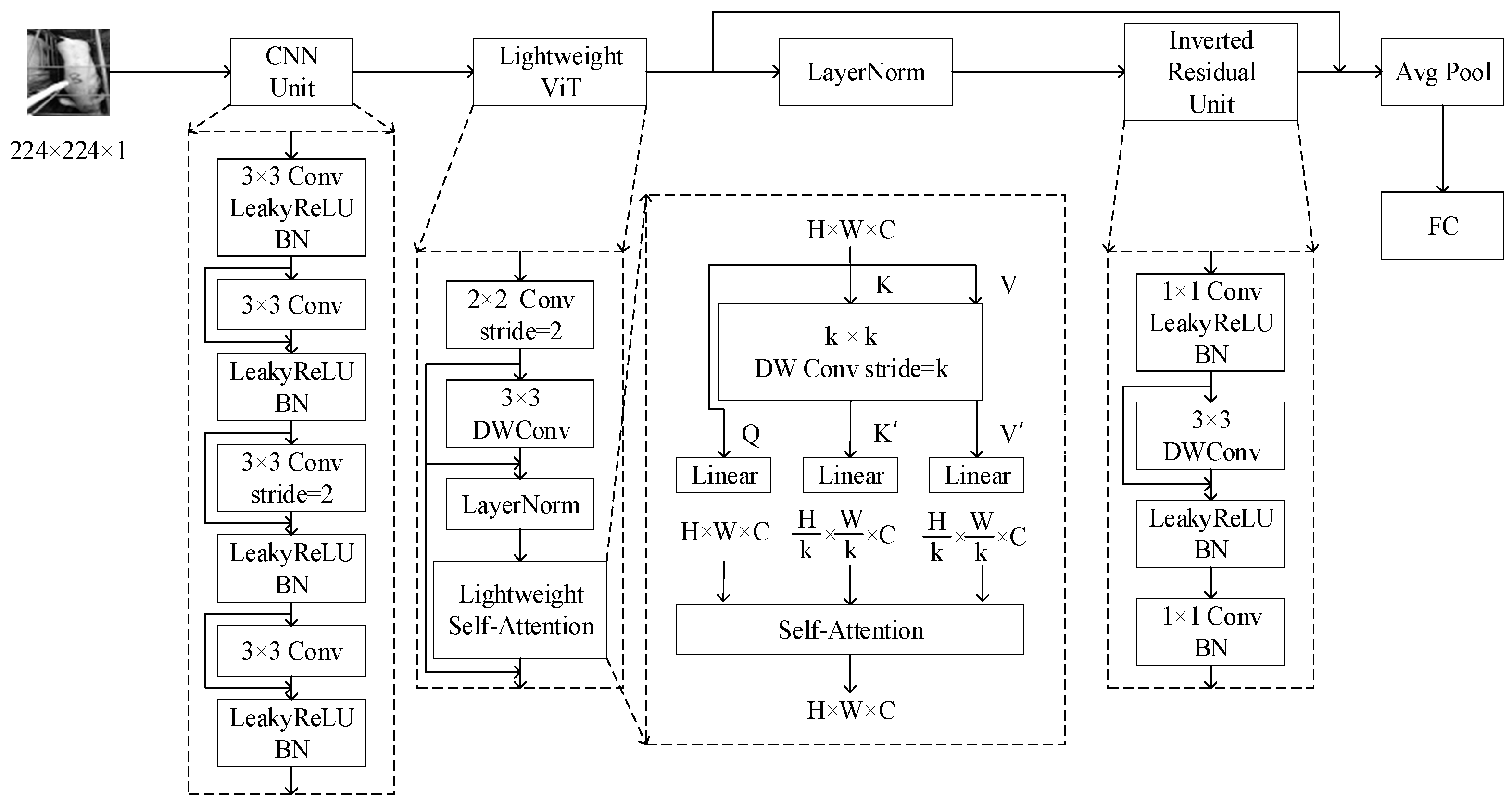
2.3. Construction of BF Measurement Model for Pregnant Sows

The CNN-ViT non-contact sows’ BF measurement model was constructed based on a CMT (Convolutional Neural Networks Meet Vision Transformers) framework [35]. The Pre-local Unit (PLU), Lightweight ViT (LViT) and Inverted Residual Unit (IRU) were included in this model. The general structure of the model is shown in Figure 5. PLU was used to reduce the image sizes of the input images and provide fine local features for the subsequent LViT. LViT was used to gather the local features extracted in the previous stage for modeling the global relationships. Then, IRU could further enhance the local information extraction of the feature maps and reduce the information loss. Finally, the class token in the original ViT was replaced by global adaptive average pooling. All features extracted by the model were integrated and sent to the fully connected layer to complete the measurement of sows’ BF.

2.3.1. Pre-Local Unit

Four convolutional layers were included in the PLU with residual connections. The residual connection was proposed to solve the problem of gradient disappearance and gradient degradation during the propagation of CNN [36]. Therefore, the residual connection was added in PLU based on the CMT framework. The basic principle of the residual connection is as follows:

$$x_{l+1}=Res\left(x_l\right)+x_l$$

(1)

where x_l+1 is the output of the l residual unit, x_l is the input of the l residual unit, and Res is the residual structure.

2.3.2. Lightweight ViT

The original ViT directly sends the blocked images into the Transformer, ignoring the local connectivity and structural information between the image blocks. Therefore, after the image was blocked, the depth-separable convolution (DWConv) with residuals was added before the Transformer. The addition of DWConv could enhance the local feature extraction within the image blocks without introducing excessive parameters and computational effort. DWConv can not only handle the spatial dimension but also the depth dimension compared to the normal convolution.

In the original ViT, the absolute position encoding was used after image blocking, which gives fixed absolute position information to each image block. This will lose the unique translation invariance of CNN and is not suitable for small datasets. Therefore, this model adopted randomly generated relative position encoding instead of absolute position encoding. Different from the objective detection, there is no need to predict the position of the sow in this task; relative position encoding can replace absolute position encoding. Moreover, relative position encoding will inject a convolution-like inductive bias into the model, which is more capable of extracting local features, more generalizable, and more suitable for smaller datasets.

After CNN extracted the local features in the previous part of the model, the self-attention mechanism computed the self-correlation within the features. Thus, the global dependencies of any two positions on the feature map can be obtained, and the global information can be fused. However, the self-attention needs to calculate the self-correlation among all the pixel points in the feature map, and the memory consumption and computational efforts are relatively large. Therefore, DWConv was introduced to downsample K and V before the attention. This can obtain features K’ and V’ with relatively small dimensionality and achieve the purpose of a lightweight Transformer. The downsampling and the lightweight self-attention combined with relative position bias after downsampling are shown as follows:

$$K^{\prime }=DWConv(K)$$

(2)

$$V^{\prime }=DWConv(V)$$

(3)

$$LightAttn(Q,K,V)=Softmax(\frac{Q{K}^{\prime T}}{\sqrt{d_k}}+B)V^{\prime }$$

(4)

where Q, K, and V are the Query, Key, and Value feature matrices obtained by linear mapping with the same dimensions as the original input, K’ and V’ are the K and V feature matrices after downsampling, d_k is the dimension of the feature, B is the relative position bias, and Softmax is the normalization function that generates attention weights.

2.3.3. Inverted Residual Unit

IRU completed dimension raising, local feature extraction, and dimension reduction by 1 × 1 convolution and DWConv. It could extract the depth of local features of the image and reduce the information loss. The operation of IRU is as follows:

$$x_{l+1}=Conv(DWConv(Conv(x_l))+Conv(x_l))$$

(5)

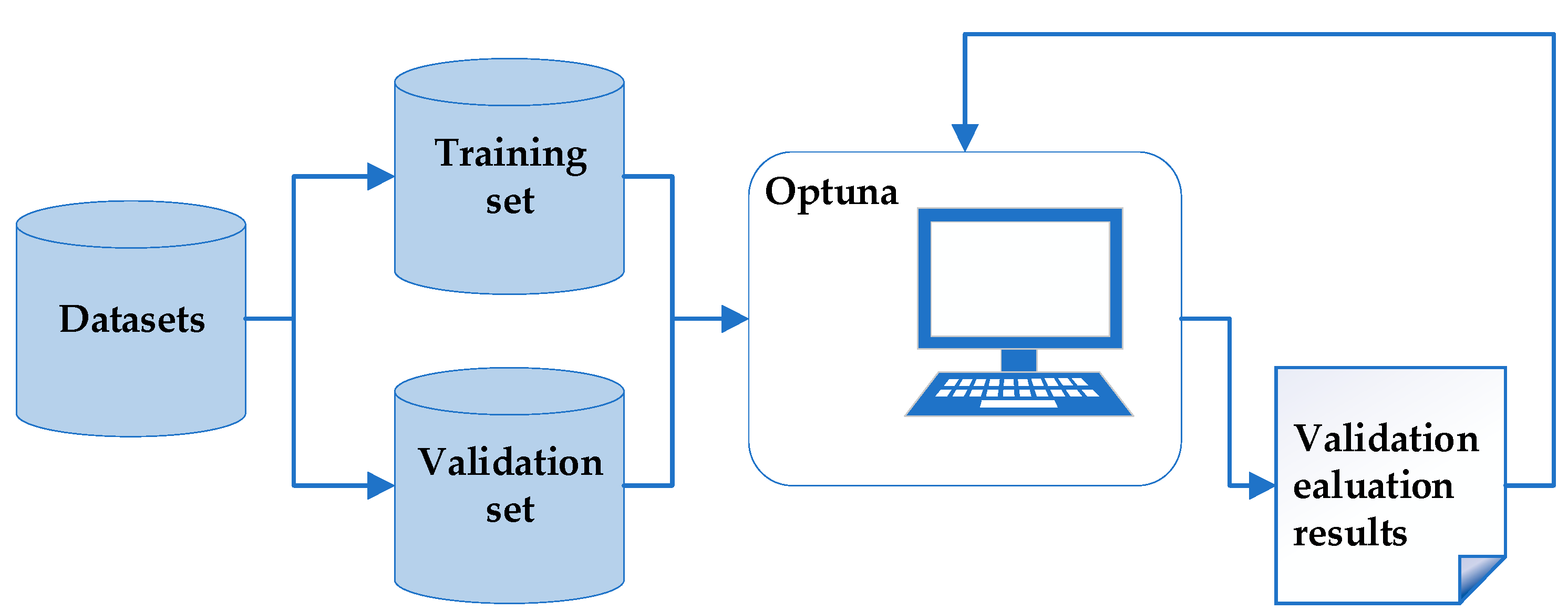
2.3.4. Hyperparameter Optimization

To make CNN-ViT more suitable for the non-contact measurement of pregnant sows’ BF, all hyperparameters of this model were optimized according to our own datasets instead of using the hyperparameters of the original CMT framework.

Compared with traditional hyperparameter optimization methods such as manual tuning and random search, automated hyperparameter optimization as a new method can automate the selection of the optimal combination of hyperparameters. As a part of AutoML (Automated Machine Learning), automated hyperparameters optimization generates the next set of suggested parameters based on the training feedback results for one set of parameters, which does not rely on subjective experience and is more efficient.

Optuna is a software framework for automatic hyperparameters optimization. By setting a range of adjustment for each hyperparameter, optuna selected the optimal hyperparameter for the model and datasets based on Bayesian optimization. The process of adjusting hyperparameters using optuna is shown in Figure 6.

The number of convolution kernels represents the number of features learned by the model from datasets. PLU is a convolutional structure located at the bottom of CNN-ViT. When the model generates more feature maps in the early stage, it has a better chance of interacting with information well in the later stage. Therefore, the range of the number of convolution kernels was set from 2 ^ 5 to 2 ^ 8 instead of using the value of the original CMT framework. In addition, the number of neurons of the fully connected layer represents the number of features used to fit the output, which directly affects the output of the model. Thus, the range of the number of neurons of the fully connected layer was also set from 2 ^ 5 to 2 ^ 8 to better fit the pregnant sows’ BF. The hyperparameters optimized by optuna and their setting ranges are shown in

Table 3. Hyperparameters optimized by optuna and their setting ranges.

Structure	Hyperparameters	Setting Ranges
PLU	Number of convolution kernels in layer 1	2 ^ 5~2 ^ 8
	Number of convolution kernels in layer 2
	Number of convolution kernels in layer 3
	Number of convolution kernels in layer 4
FC	Number of features

.

Considering the relatively small dataset, the PLU, LViT, and IRU values in the CNN-ViT model were all only one and not stacked in order to prevent overfitting. Similarly, the number of heads of attention was set to 1. The other hyperparameters of CNN-ViT were the same as those in the CMT framework. The hyperparameters of the CNN-ViT pregnant sows’ BF measurement model are shown in

Table 4. CNN-ViT network parameters for non-contact measurement of pregnant sows.

Structure	Hyperparameters	Values
PLU	Number of convolution kernels in layer 1	128
	Number of convolution kernels in layer 2	32
	Number of convolution kernels in layer 3	256
	Number of convolution kernels in layer 4	256
LViT	Dimension of image block flattening	46
	Number of heads of attention	1
	Lightweight dimension of attention k	8
IRU	Proportion of dimensional raising	3.6
	Proportion of dimensional reduction	3.6
FC	Number of features	128

.

2.4. Model Training and Performance Evaluation

2.4.1. Training Environment

In this study, the model was trained based on the Windows 10 operating system. The GPU was an NVIDIA GeForce RTX 3090Ti, and the Cuda version was 11.3. The programming language used was Python 3.9.0, and the deep learning framework was PyTorch 1.11.0.

The number of epochs was set to 30, the optimizer used Adaptive Moment Estimation (Adam), the batch size was 16, and the initial learning rate was 0.001. The multi-step decay strategy was adopted, which can be calculated as follows:

$$lr=\left\{\begin{array}{l}l{r}_{0}epoch<epochs\times \frac{1}{2}\\ 0.1\times l{r}_{0}epochs/2\le epoch<epochs\times \frac{3}{4}\\ 0.01\times l{r}_{0}epoch\ge epochs\times \frac{3}{4}\end{array}\right.$$

(6)

where lr₀ is the initial learning rate, epoch is the current epoch, and epochs is the total number of epochs.

The Mean Square Error Loss (MSELoss) function was used to measure the degree of difference between the predicted and true values of the sows’ BF during the training process.

2.4.2. Evaluation Indicators

In this study, the Mean Absolute Error (MAE), Mean Square Error (MSE), Root Mean Square Error (RMSE), Mean Absolute Percentage Error (MAPE) and R-Square (R²) were selected as the evaluation indicators of the BF measurement model.

3. Results and Discussion

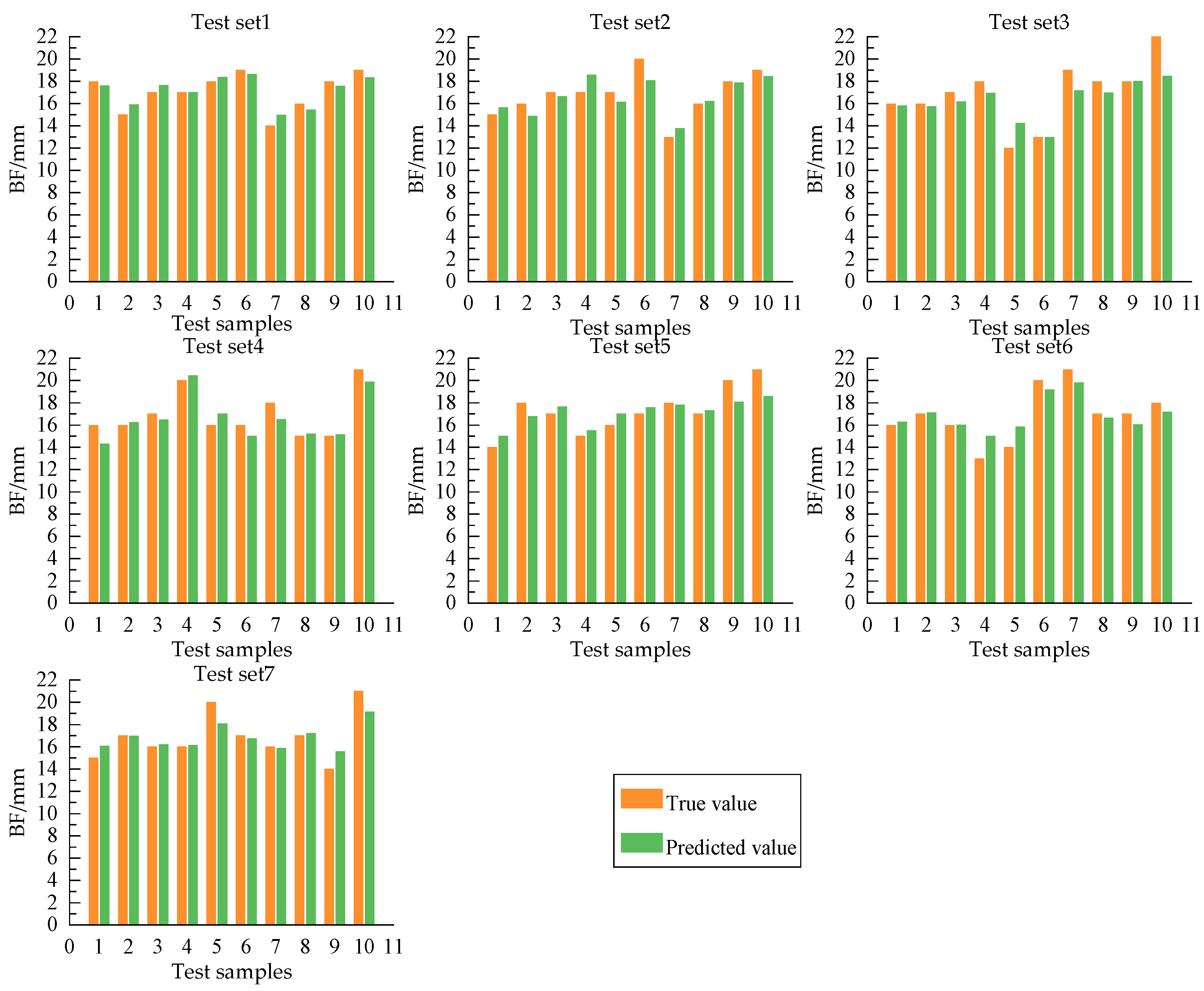
3.1. Test Results of CNN-ViT

Median filtering was applied to the predicted BF of 90 images for each sample in the test set, and this was used as the test result. The test results on the seven test sets are shown in Table 4. A comparison of the predicted and true values of the model on each test set is shown in Figure 5. The MAE of the CNN-ViT model was 0.83 mm, the RMSE was 1.05 mm, the MAPE was 4.87%, and the R² was 0.74. The results showed that the CNN-ViT had high accuracy and generalization ability.

Combined with

Table 5. Performance of CNN-ViT model on different test sets.

Test Set	MAE/mm	RMSE/mm	MAPE/%	R2
1	0.53	0.60	3.24	0.86
2	0.81	0.98	4.82	0.73
3	1.10	1.54	6.38	0.68
4	0.79	0.94	4.58	0.77
5	0.98	1.19	5.48	0.65
6	0.84	1.07	5.34	0.78
7	0.74	1.04	4.28	0.73
AVG	0.83	1.05	4.87	0.74

and Figure 7, test set 1 reached the best result among the seven test sets with an MAE of 0.53 mm, RMSE of 0.60 mm, MAPE of 3.24%, and R² of 0.86. The distribution of true BF values in test set 1 was more concentrated. The minimum true BF and maximum true BF in test set 1 were greater and less than those in the rest of the test set, respectively. Test set 3 had a larger test error with an MAE of 1.10 mm, RMSE of 1.54 mm, MAPE of 6.38% and R² of 0.68. The reason might be the scattered true BF values in the test samples of this test set. The minimum true BF and maximum true BF in test set 3 were both extreme values in all test samples and were proportionally smaller in the overall samples. The model training did not learn as sufficiently for fewer samples as other samples, so it was prone to poor prediction and larger errors for extreme samples in test set 3.

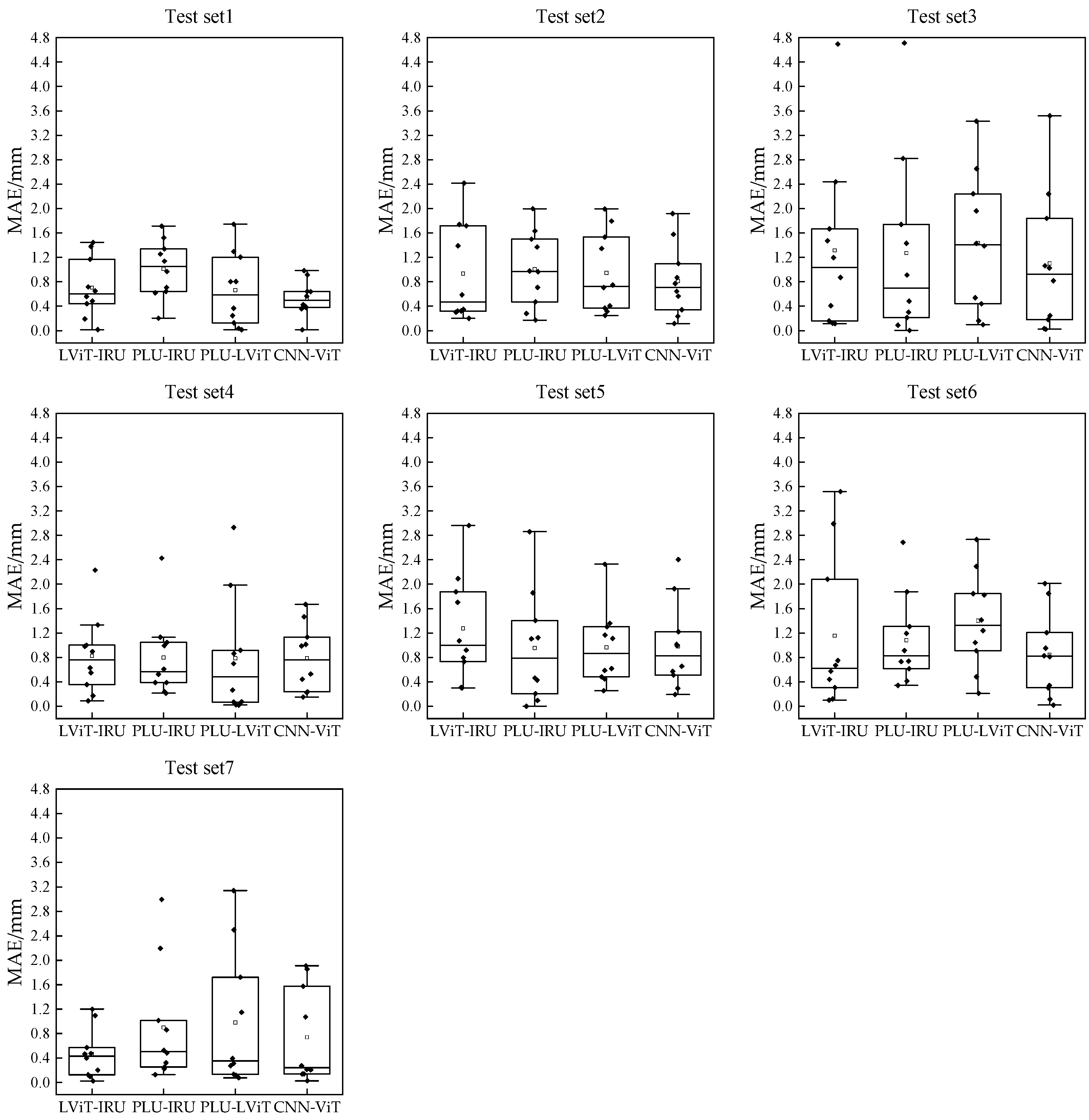
3.2. Comparative Analysis Based on Different Structural Models

To verify the usefulness of PLU, LViT and IRU in the CNN-ViT, three different structural models of LViT-IRU, PLU-IRU and PLU-LViT were constructed for comparison, respectively. The average test results of each model with seven test sets are shown in

Table 6. Comparison of the performance of different structural models.

Model	MAE ± SE/mm	RMSE ± SE/mm	MAPE ± SE/%	R2 ± SE	Params/M	FLOPs/G
LViT-IRU	0.95 ± 0.11	1.24 ± 0.16	5.75 ± 0.69	0.63 ± 0.06	2.50	0.38
PLU-IRU	1.00 ± 0.05	1.29 ± 0.10	5.93 ± 0.38	0.61 ± 0.03	1.79	24.09
PLU-LViT	1.02 ± 0.10	1.31 ± 0.11	6.12 ± 0.67	0.60 ± 0.03	1.00	11.60
PLU-LViT-IRU (CNN-ViT)	0.83 ± 0.06	1.05 ± 0.10	4.87 ± 0.35	0.74 ± 0.02	0.39	3.85

. The error distribution on each test set is shown in Figure 8.

CNN-ViT with PLU, LViT and IRU achieved the best performance compared to the other comparison models, and the error was smaller for each test set. Compared with other models, the MAE of CNN-ViT decreased by more than 12%, the RMSE decreased by more than 15%, the MAPE decreased by more than 15%, and R² improved by more than 17%. In addition, CNN-ViT contained three modules, and the model had the smallest number of parameters, with 0.39 M.

Compared with LViT-IRU and CNN-ViT, CNN-ViT showed a 12.63% lower MAE, 15.32% lower RMSE, 15.30% lower MAPE, and 17.64% higher R² than LViT-IRU with a higher accuracy and generalization ability. This indicated that the PLU located at the head of the CNN-ViT could help improve the performance of the model. The PLU with a CNN structure was used to extract local features of images with translation invariance, which could provide a priori knowledge to the model such as inductive bias. Although PLU would significantly increase the FLOPs of model, the addition of the PLU before ViT could provide more refined local features for it and reduce the input image size, reducing the number of model parameters. Moreover, the residual structure was introduced in the PLU, which could better retain the features extracted from the images.

Compared with PLU-LRU and CNN-ViT, CNN-ViT showed a 17.00% lower MAE, 18.60% lower RMSE, 17.88% lower MAPE, and 21.31% better R² than PLU-LRU with higher accuracy and better fitting of the data. The CNN structure on its own had limitations in establishing relationships between global information. The self-attention could extract global features from the images to compensate for its shortcomings. Therefore, the combination of both could obtain more comprehensive and sufficient features. Additionally, this model added DWConv after image blocking and used lightweight self-attention. This enhanced the information interaction between image blocks and reduced the number of model parameters, making it more possible to obtain better results even on small datasets.

Compared with PLU-LViT and CNN-ViT, CNN-ViT showed a 18.63% lower MAE, 19.85% lower RMSE, 20.42% lower MAPE, and 23.33% higher R² than PLU-LViT. IRU was used after LViT to integrate all the features extracted in the first stage of the model. Nonlinear transformation was performed on these features to complete the interaction of information between them, which improved the feature representation ability of the network. IRU had a positive effect on the model and was an indispensable part of CNN-ViT.

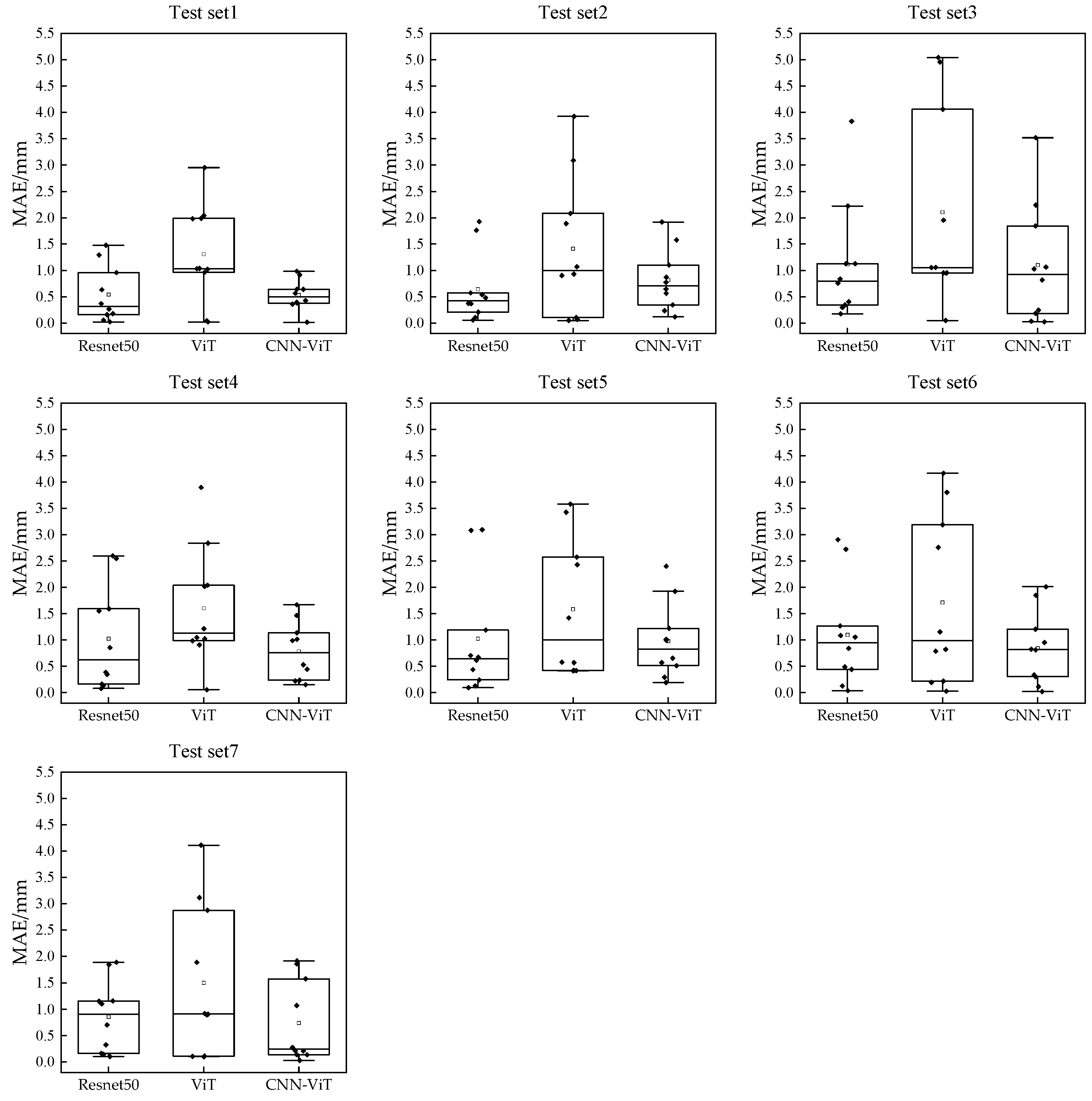
3.3. Comparative Analysis Based on Different Deep Learning Models

To further validate the performance of the CNN-ViT for measuring sows’ BF, Resnet50, a representative model of the full CNN structure, and ViT, a representative model of the full Transformer structure, were used as comparison models. The results of BF measurements for different models are shown in

Table 7. Comparison of the performance of different deep learning models.

Model	MAE ± SE/mm	RMSE ± SE/mm	MAPE ± SE/%	R2 ± SE	Params/M	FLOPs/G
Resnet50	0.90 ± 0.08	1.22 ± 0.11	5.28 ± 0.44	0.64 ± 0.05	23.50	4.05
ViT	1.60 ± 0.09	2.06 ± 0.13	9.69 ± 0.65	0.01 ± 0.00	51.49	2.57
CNN-ViT	0.83 ± 0.06	1.05 ± 0.10	4.87 ± 0.35	0.74 ± 0.02	0.39	3.85

. The error distribution on each test set is shown in Figure 9.

CNN-ViT achieved the best performance compared to Resnet50 and ViT. Compared with other models, the MAE of CNN-ViT decreased by more than 7%, the RMSE decreased by more than 13%, the MAPE decreased by more than 7%, and R² improved by more than 15%. Moreover, the parameters of CNN-ViT in this study were only 0.39M, which was far lower than Resnet50 and ViT and more suitable for small datasets and hardware embedding.

Compared with Resnet50, the MAE, RMSE, and MAPE of the CNN-ViT were decreased by 7.78%, 13.93%, and 7.77%, respectively, and the R² was improved by 15.63%. CNN-ViT had higher measurement accuracy and a better model-fitting ability. Compared with traditional CNN, adding the ViT structure to the model could make it learn the global semantic information of images more effectively so that it would not be limited to the local perceptual properties of convolution. In addition, the self-attention in the ViT could dynamically adjust the perceptual domain, which had better robustness to the interference and noise in the images [37]. For the dataset used in this study, self-attention could reduce the effect of the occlusion of the pig pen within the image background on the prediction accuracy.

Compared with ViT, the MAE, RMSE, and MAPE of CNN-ViT were decreased by 48.13%, 49.03%, and 49.74%, respectively, and R² was improved by 7300%. On this study dataset, the R² of ViT was 0.01 with no ability to measure BF and fit the dataset. This was due to ViT’s lack of inductive bias ability of convolution, which required a huge amount of data as a support to achieve better performance than CNN. The number of FLOPs of ViT was the lowest with 2.57G, but ViT had difficulty achieving good results without using pre-trained models or being directly applied on small datasets.

4. Conclusions and Future Work

To address the problems of the high intensity caused by the traditional contact measurement of sows’ BF, the low efficiency of existing non-contact measurement BF models and the insufficient global feature extraction ability of the CNN, we proposed a non-contact measurement model based on CNN-ViT for pregnant sows’ BF by using the images of the back of pregnant sows from a top view. CNN-ViT was tested, and a comparative analysis was carried out with different structural models such as LViT-IRU, PLU-IRU and PLU-LViT and different deep learning models such as Resnet50 and ViT. The main conclusions from this study are as follows:

• The MAE of CNN-ViT on the seven randomly divided test sets was 0.83 mm, the RMSE was 1.05 mm, the MAPE was 4.87%, and R² was 0.74. The model could complete the non-contact measurement of sows’ BF with relatively high accuracy and generalization.
• Compared with different structural models (LViT-IRU, PLU-IRU and PLU-LViT) and different deep learning models (Resnet50 and ViT), the CNN-ViT model performed better.

Based on the results obtained, the proposed approach could undoubtedly contribute to the non-contact measurement of pregnant sows’ BF. However, the dataset contained only 106 pregnant sow samples, and more samples should be collected to build a larger dataset for model accuracy promotion. Additionally, the image pre-processing method should be more refined to further improve image quality.

References

1. Hu, J.; Yan, P. Effects of Backfat Thickness on Oxidative Stress and Inflammation of Placenta in Large White Pigs. Vet. Sci. 2022, 9, 302. [Google Scholar] [CrossRef] [PubMed]
2. Zhou, Y.; Xu, T.; Cai, A.; Wu, Y.; Wei, H.; Jiang, S.; Peng, J. Excessive backfat of sows at 109 d of gestation induces lipotoxic placental environment and is associated with declining reproductive performance. J. Animal Sci. 2018, 96, 250–257. [Google Scholar] [CrossRef] [PubMed]
3. Li, J.-W.; Hu, J.; Wei, M.; Guo, Y.-Y.; Yan, P.-S. The Effects of Maternal Obesity on Porcine Placental Efficiency and Proteome. Animals 2019, 9, 546. [Google Scholar] [CrossRef] [PubMed] [Green Version]
4. Superchi, P.; Saleri, R.; Menčik, S.; Dander, S.; Cavalli, V.; Izzi, C.; Ablondi, M.; Sabbioni, A. Relationships among maternal backfat depth, plasma adipokines and the birthweight of piglets. Livest. Sci. 2019, 223, 138–143. [Google Scholar] [CrossRef]
5. Roongsitthichai, A.; Koonjaenak, S.; Tummaruk, P. Backfat Thickness at First Insemination Affects Litter Size at Birth of the First Parity Sows. Agric. Nat. Resour. 2010, 44, 1128–1136. [Google Scholar]
6. Thongkhuy, S.; Chuaychu, S.B.; Burarnrak, P.; Ruangjoy, P.; Juthamanee, P.; Nuntapaitoon, M.; Tummaruk, P. Effect of backfat thickness during late gestation on farrowing duration, piglet birth weight, colostrum yield, milk yield and reproductive performance of sows. Livest. Sci. 2020, 234, 103983. [Google Scholar] [CrossRef]
7. Koketsu, Y.; Takahashi, H.; Akachi, K. Longevity, Lifetime Pig Production and Productivity, and Age at First Conception in a Cohort of Gilts Observed over Six Years on Commercial Farms. J. Vet. Med. Sci. 1999, 61, 1001–1005. [Google Scholar] [CrossRef] [Green Version]
8. Liu, B.; Chen, Y.; Jiang, X.; Guo, Z.; Zhong, Z.; Zhang, S.; Zhu, L. Effect of backfat thickness on body condition score and reproductive performance of sows during pregnancy. Acta Agric. Zhejiangensis 2020, 32, 390–397. [Google Scholar]
9. Zhao, Y.X.; Yang, W.P.; Tao, R.J.; Li, Z.Y.; Zhang, C.L.; Liu, X.H.; Chen, Y.S. Effect of backfat thickness during pregnancy on farrowing duration and reproductive performance of sows. China Anim. Husb. Vet. Med. 2019, 46, 1397–1404. [Google Scholar]
10. Fisher, A.V. A review of the technique of estimating the composition of livestock using the velocity of ultrasound. Comput. Electron. Agric. 1997, 17, 217–231. [Google Scholar] [CrossRef]
11. Ginat, D.T.; Gupta, R. Advances in Computed Tomography Imaging Technology. Annu. Rev. Biomed. Eng. 2014, 16, 431–453. [Google Scholar] [CrossRef] [PubMed]
12. Sharma, S.; Mittal, R.; Goyal, N. An Assessment of Machine Learning and Deep Learning Techniques with Applications. ECS Trans. 2022, 1, 107. [Google Scholar] [CrossRef]
13. Teng, G.; Shen, Z.; Zhang, J.; Shi, C.; Yu, J. Non-contact sow body condition scoring method based on Kinect sensor. Trans. Chin. Soc. Agric. Eng. 2018, 34, 211–217. [Google Scholar]
14. Araujo Fernandes, A.F.; Dorea, J.; Valente, B.; Fitzgerald, R.; Herring, W.; Rosa, G. Comparison of data analytics strategies in computer vision systems to predict pig body composition traits from 3D images. J. Anim. Sci. 2020, 98, skaa250. [Google Scholar] [CrossRef]
15. Zuo, C.; Zhang, X.; Hu, Y.; Yin, W.; Shen, D.; Zhong, J.; Zheng, J.; Chen, Q. Has 3D finally come of age?—An introduction to 3D structured-light sensor. Infrared Laser Eng. 2020, 49, 9–53. [Google Scholar]
16. Xiao, Z.; Zhou, M.; Yuan, H.; Liu, Y.; Fan, C.; Cheng, M. Influence Analysis of Light Intensity on Kinect v2 depth measurement accuracy. Trans. Chin. Soc. Agric. Mach. 2021, 52, 108–117. [Google Scholar]
17. Yu, M.; Zheng, H.; Xu, D.; Shuai, Y.; Tian, S.; Cao, T.; Zhou, M.; Zhu, Y.; Zhao, S.; Li, X. Non-contact detection method of pregnant sows backfat thickness based on two-dimensional images. Anim. Genet. 2022, 53, 769–781. [Google Scholar] [CrossRef]
18. Rodríguez Alvarez, J.; Arroqui, M.; Mangudo, P.; Toloza, J.; Jatip, D.; Rodríguez, J.M.; Teyseyre, A.; Sanz, C.; Zunino, A.; Machado, C. Body condition estimation on cows from depth images using Convolutional Neural Networks. Comput. Electron. Agric. 2018, 155, 12–22. [Google Scholar] [CrossRef] [Green Version]
19. Yukun, S.; Pengju, H.; Yujie, W.; Ziqi, C.; Yang, L.; Baisheng, D.; Runze, L.; Yonggen, Z. Automatic monitoring system for individual dairy cows based on a deep learning framework that provides identification via body parts and estimation of body condition score. J. Dairy Sci. 2019, 102, 10140–10151. [Google Scholar] [CrossRef]
20. Zhao, K.; Zhang, M.; Shen, W.; Liu, X.; Ji, J.; Dai, B.; Zhang, R. Automatic body condition scoring for dairy cows based on efficient net and convex hull features of point clouds. Comput. Electron. Agric. 2023, 205, 107588. [Google Scholar] [CrossRef]
21. Shi, W.; Dai, B.; Shen, W.; Sun, Y.; Zhao, K.; Zhang, Y. Automatic estimation of dairy cow body condition score based on attention-guided 3D point cloud feature extraction. Comput. Electron. Agric. 2023, 206, 107666. [Google Scholar] [CrossRef]
22. Lv, P.; Wu, W.; Zhong, Y.; Du, F.; Zhang, L. SCViT: A Spatial-Channel Feature Preserving Vision Transformer for Remote Sensing Image Scene Classification. IEEE Trans. Geosci. Remote Sens. 2022, 60, 4409512. [Google Scholar] [CrossRef]
23. Moutik, O.; Sekkat, H.; Tigani, S.; Chehri, A.; Rachid, S.; Ait Tchakoucht, T.; Paul, A. Convolutional Neural Networks or Vision Transformers: Who Will Win the Race for Action Recognitions in Visual Data? Sensors 2023, 23, 734. [Google Scholar] [CrossRef] [PubMed]
24. Dosovitskiy, A.; Beyer, L.; Kolesnikov, A.; Weissenborn, D.; Zhai, X.; Unterthiner, T.; Dehghani, M.; Minderer, M.; Heigold, G.; Gelly, S.; et al. An Image is Worth 16 × 16 Words: Transformers for Image Recognition at Scale. In Proceedings of the International Conference on Learning Representations(ICLR), Vienna, Austria, 4 May 2021. [Google Scholar]
25. Hou, R.; Chen, J.; Feng, Y.; Liu, S.; He, S.; Zhou, Z. Contrastive-weighted self-supervised model for long-tailed data classification with vision transformer augmented. Mech. Syst. Signal Process. 2022, 177, 109174. [Google Scholar] [CrossRef]
26. Park, S.; Kim, G.; Oh, Y.; Seo, J.B.; Lee, S.M.; Kim, J.H.; Moon, S.; Lim, J.-K.; Park, C.M.; Ye, J.C. Self-evolving vision transformer for chest X-ray diagnosis through knowledge distillation. Nat. Commun. 2022, 13, 3848. [Google Scholar] [CrossRef]
27. Dhanya, V.G.; Subeesh, A.; Kushwaha, N.L.; Vishwakarma, D.K.; Nagesh Kumar, T.; Ritika, G.; Singh, A.N. Deep learning based computer vision approaches for smart agricultural applications. Artif. Intell. Agric. 2022, 6, 211–229. [Google Scholar] [CrossRef]
28. Touvron, H.; Cord, M.; Douze, M.; Massa, F.; Sablayrolles, A.; Jégou, H. Training data-efficient image transformers & distillation through attention. In Proceedings of the International Conference on Machine Learning (ICML), Electr Network, Online, 18–24 July 2021. [Google Scholar]
29. Han, K.; Wang, Y.; Chen, H.; Chen, X.; Guo, J.; Liu, Z.; Tang, Y.; Xiao, A.; Xu, C.; Xu, Y.; et al. A Survey on Vision Transformer. IEEE Trans. Pattern Anal. Mach. Intell. 2023, 45, 87–110. [Google Scholar] [CrossRef] [PubMed]
30. Verma, V.; Gupta, D.; Gupta, S.; Uppal, M.; Anand, D.; Ortega-Mansilla, A.; Alharithi, F.S.; Almotiri, J.; Goyal, N. A Deep Learning-Based Intelligent Garbage Detection System Using an Unmanned Aerial Vehicle. Symmetry 2022, 14, 960. [Google Scholar] [CrossRef]
31. Mishra, A.; Harnal, S.; Mohiuddin, K.; Gautam, V.; Nasr, O.; Goyal, N.; Alwetaishi, M.; Singh, A. A Deep Learning-based Novel Approach for Weed Growth Estimation. Intell. Autom. Soft Comput. 2022, 2, 1157–1173. [Google Scholar] [CrossRef]
32. Greer, E.; Mort, P.; Lowe, T.; Giles, L. Accuracy of ultrasonic backfat testers in predicting carcass P2 fat depth from live pig measurement and the effect on accuracy of mislocating the P2 site on the live pig. Aust. J. Exp. Agric. 1987, 27, 27. [Google Scholar] [CrossRef]
33. Vakharia, V.; Shah, M.; Nair, P.; Borade, H.; Sahlot, P.; Wankhede, V. Estimation of Lithium-ion Battery Discharge Capacity by Integrating Optimized Explainable-AI and Stacked LSTM Model. Batteries 2023, 9, 125. [Google Scholar] [CrossRef]
34. Mayrose, H.; Bairy, G.M.; Sampathila, N.; Belurkar, S.; Saravu, K. Machine Learning-Based Detection of Dengue from Blood Smear Images Utilizing Platelet and Lymphocyte Characteristics. Diagnostics 2023, 13, 220. [Google Scholar] [CrossRef] [PubMed]
35. Guo, J.; Han, K.; Wu, H.; Tang, Y.; Chen, X.; Wang, Y.; Xu, C. CMT: Convolutional Neural Networks Meet Vision Transformers. In Proceedings of the IEEE/CVF Conference on Computer Vision and Pattern Recognition (CVPR), New Orleans, LA, USA, 18–24 June 2022. [Google Scholar]
36. He, K.; Zhang, X.; Ren, S.; Sun, J.; He, K.; Zhang, X.; Ren, S.; Sun, J. Deep Residual Learning for Image Recognition. In Proceedings of the IEEE/CVF Conference on Computer Vision and Pattern Recognition (CVPR), Las Vegas, NV, USA, 27–30 June 2016. [Google Scholar]
37. Naseer, M.; Ranasinghe, K.; Khan, S.; Hayat, M.; Khan, F.S.; Yang, M.-H. Intriguing Properties of Vision Transformers. In Proceedings of the Neural Information Processing Systems (NeurIPS), Electr Network, Virtual, 6–14 December 2021. [Google Scholar]
Figure 1. CNN-ViT for non-contact measurement of pregnant sows’ BF.
Agriculture 13 01395 g001
Figure 2. Flowchart for cropping each sample.
Agriculture 13 01395 g002
Figure 3. Comparison of the data before and after pre-processing; (a) refers to the original RGB image before cropping, and (b) refers to the grayscale image after cropping.
Agriculture 13 01395 g003
Figure 4. Sample distribution by body condition score and gestation periods.
Agriculture 13 01395 g004
Figure 5. Structure of CNN-ViT feature map measurement model for pregnant sows.
Agriculture 13 01395 g005
Figure 6. Process of adjusting hyperparameters using optuna.
Agriculture 13 01395 g006
Figure 7. Comparison of the predicted and true values for CNN-ViT.
Agriculture 13 01395 g007
Figure 8. Comparison of test error based on different structural models.
Agriculture 13 01395 g008
Figure 9. Comparison of test error based on different deep learning models.
Agriculture 13 01395 g009