The Use of Hough Transform Method and Knot-Like Turning for Motion Planning and Control of an Autonomous Agricultural Vehicle

Abstract

This study focuses on motion planning and reference trajectory tracking control of an autonomous agricultural vehicle to achieve precise row following and turning. The smooth time-varying feedback control method was adapted to the system to generate the required control commands. The mathematical representations for motion planning and controllers were constructed based on the car-like robot model. An algorithm to detect trees and rows of trees of an orchard was developed using the Hough transform approach. A new type of turning procedure, called knot-like turning, was proposed to perform turning from one row to another. A simulation environment was created to test and analyze the developed system. To obtain the real data from a field, the trees and rows of trees of a cherry orchard were scanned using a laser scanner rangefinder sensor. Then, the scanned data were moved to the simulation environment to generate the desired trajectory, which was followed by an autonomous agricultural vehicle. The simulation environment made it possible to determine the performance of the proposed motion planning, reference trajectory generation, tracking control and turning procedures. The results presented here indicate that the proposed methodology could be used for desired trajectory tracking tasks for agricultural operations in the case that minimum tracking errors in both straight and turning motions are needed.

1. Introduction

Autonomous systems have been rapidly growing and used in industry for the last two decades. The developments and enhancements gained in autonomous systems, equipment, methods and approaches have also been adapting to agricultural systems. Agricultural systems must be automated, since the world’s population is significantly increasing, and people need more agricultural products. Agricultural applications and operations should be automatically controlled in order to meet these expectations.

With the recent developments in autonomous control in agricultural operations, mechatronics systems are being used together with agricultural tools in an efficient manner. This collaboration can be expected to continue growing in the near future.

This paper presents a methodology that combines four main issues. The first issue was about motion planning and desired trajectory generation for the autonomous agricultural vehicle applications. Reference trajectory and motion planning, which are specified according to a task, were modeled and created based on the car-like robot approach. The second issue was the development control strategies for the steering and driving systems of the vehicle. To generate these control commands, the smooth time-varying feedback control procedure was used and adapted into the proposed system. The third issue was the development of a methodology to conduct the operations of detection of trees and estimation of rows of trees. The methodology was built by following the principles of the Hough transform method. The last issue was to build a turning strategy to perform turning from one row of trees to another. A new type of turning geometry, called knot-like turning, was proposed. It is considered that knot-like turning methodology is useful when there is a limited spare space for turning, and precise row following is the main objective. In order to test the performance of the developed algorithms and methodologies, a simulation environment was created, and a number of simulation studies were conducted.

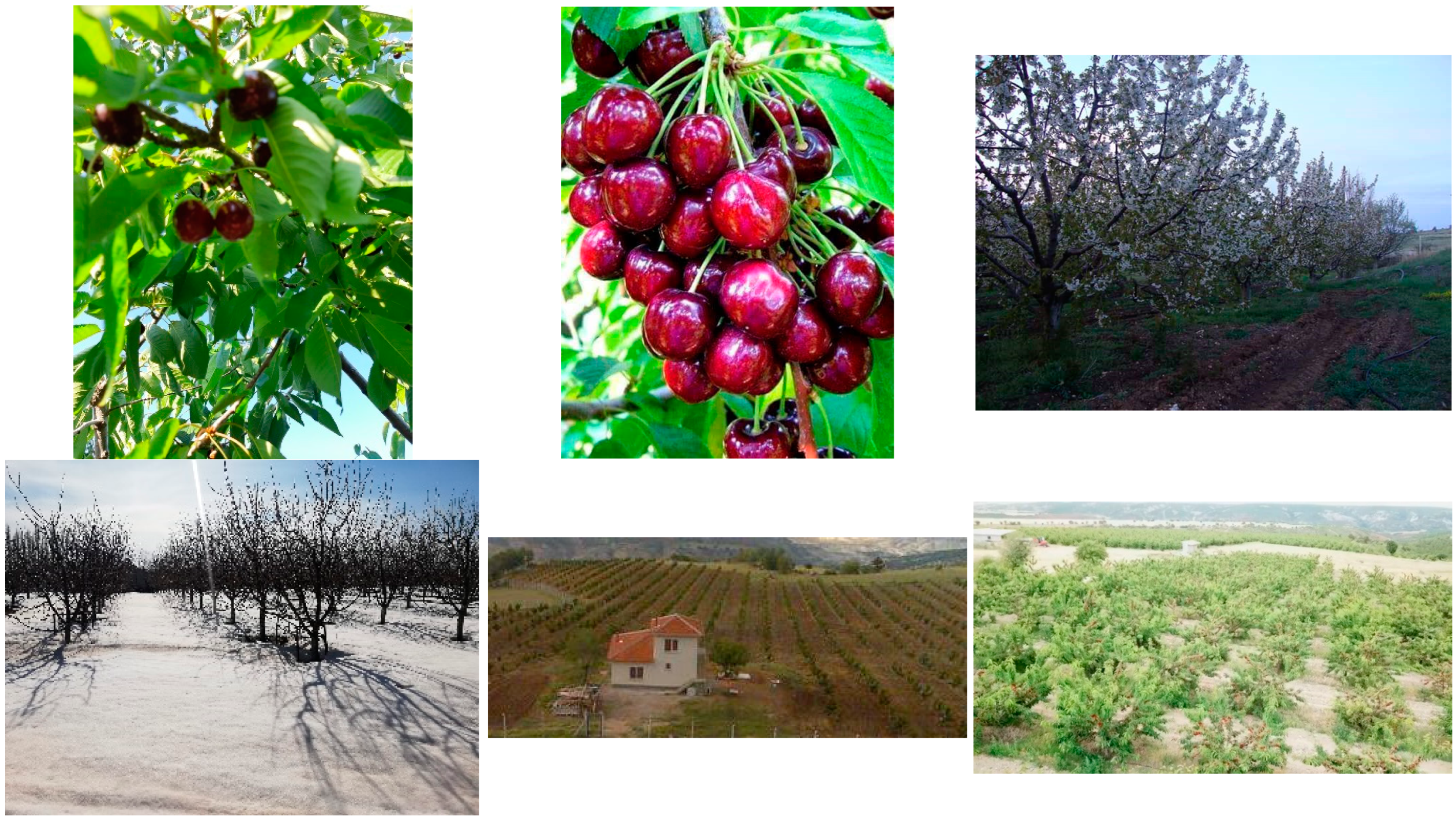
The Mihaliccik region of Turkey (Eskisehir) (39°51′34.3″ N 31°31′35.4″ E) a well-known place due to its cherry orchards. This region allows the growers to yield high-quality Napoleon cherries, one of the most famous cherry types in the cherry family. The amount of cherry production is rapidly increasing every year. To keep pace with this rise in cherry production, the growers have used autonomous systems in their orchard operations, e.g., the use of autonomous vehicles, robotic systems, etc. As the scope of this study, the trees and rows of trees of one of the cherry orchards in this region were scanned using a mid-range laser scanner rangefinder. Then, the scanned data were moved to the developed simulation environment. In addition to detecting trees, estimating rows of trees and creating reference trajectories (the center line between two consecutive rows of trees), the simulation environment was used to examine a four-wheeled orchard vehicle’s behavior during straight and turning motions. The simulation environment also provided opportunities for testing the performance, efficiency, robustness and repeatability of the proposed control system. The details of the mathematical background of the procedures proposed and the results of simulation studies are presented in this paper.

This paper is organized as follows. The next section discusses related works. The Material and Methods section includes seven subsections: the problem statement, generation of desired trajectory, design steps of the feedback controller, turning procedure proposed in this study, cherry orchard where the trees and rows of trees were scanned using a laser scanner range finder, tree detection procedure and details of row estimation procedure constructed based on the Hough transform method. Prior to the conclusion, the Results and Discussion sections are presented.

Related Works

The problems encountered during autonomous driving in an orchard environment can be divided into the following subproblems: the control of the position and orientation of the vehicle, navigation, trajectory generation/path planning, the detection of trees and estimation of rows of trees, and building the turning path.

The control of nonholonomic-wheeled robots in motion on a plane was studied by the authors of [1], who used feedback control techniques for performing trajectory tracking tasks. This study can be used to model autonomous robot/vehicle applications. The modeling structure proposed in the present study was also guided by this approach. A new path-tracking control for a car-like robot was presented [2]. The control system was constructed using neural predictive control procedure. The study was tested for only indoor applications. The parking problem of a car-like mobile robot was studied by the authors of [3], who focused on the stabilization problem of nonholonomic systems. A simple and efficient methodology for stability analysis was introduced. Turning strategies, which are adaptable to autonomous vehicle applications, were also introduced. The motion control of wheeled mobile robots was investigated [4]. The dynamic feedback linearization technique was used for solving trajectory tracking and set-point regulation problems. The presented system was tested using an indoor mobile robot. Nonlinear trajectory tracking control for a car-like robot was studied [5]. The controller was constructed based on the dynamic feedback linearization method. The modeling structures presented by the authors of [4,5] can be adapted for indoor autonomous trajectory tracking applications. The details of the modeling of the trajectory generation, path planning and tracking controllers for autonomous vehicles were given by the authors of [6]. Different types of approaches for controller design were introduced (the presented approaches were also taken into consideration in the modeling part of this paper). A solution procedure for path tracking problem of a mobile robot was proposed [7]. A robust PID controller was adapted to the system for achieving accurate path tracking. A car-like robot model was used for reference trajectory generation for an autonomous tractor [8]. A nonlinear adaptive controller was designed for both achieving trajectory tracking and rejecting sliding effects. The introduced system was not tested for real orchard applications.

An autonomous navigation system for an orchard vehicle was introduced [9]. The system uses a laser scanner rangefinder. It detects trees and estimates rows of trees using the principles of the Hough transform technique. The proposed system does not address turning from one row to another. Moreover, the turning strategy, mathematical representation and adaptation were not provided. A low-cost localization and navigation methodology was proposed for autonomous vineyard sprayer robots [10]. A data fusion technique that processed the data from various sensors was also introduced. Instead of using a laser scanner, the system uses the visual odometry based on the orchard video data. The motion model of the autonomous vehicle was constructed based on the kinematic approach. The researchers did not focus on a desired trajectory generator, feedback controller or plant detection system.

Trajectory tracking problems for autonomous farming vehicles were studied [11]. A combination of nonlinear and sliding mode controllers was used to create a curved path tracking system. A simple U-turn method was presented. The performance of the controller during tracking the U-shaped desired trajectory was illustrated. The authors of [12] stated the accurate localization of autonomous vehicles in orchard environment depends on how precisely the orchard map is built. To verify this statement, a methodology to create a local orchard map based on the combination of camera and laser scanner data was proposed. The system also introduced a simple tree trunk detection algorithm. A motion model was constructed using a prediction-correction model. U-shaped turning was used for performing turnings between rows. A laser scanning rangefinder sensor model was constructed for performing autonomous navigation of a robot [13]. The identification of the robot’s surrounding was achieved using an algorithm constructed based on the particle filter. The system does not involve a feedback controller. Therefore, the tracking performance was not provided. The performances of the particle filter and localization were not shown for a turning operation. An image-based particle filtering technique was developed and used to perform localization in an agricultural environment [14]. The proposed system obtained the uncertainties for increasing robustness in autonomous navigation. It did not involve a closed-loop control system. To achieve turning between rows of trees, a simple U-shaped turning trajectory was used. Different headland turning techniques using continuous curvature paths were proposed [15]. The turning shapes introduced were tested for cases where the turning was coupled with the motion model, which was constructed based on a car-like robot approach. The desired trajectory generation technique and feedback control design were not presented. A new methodology for generating curvature trajectory for agricultural vehicles was introduced [16]. The forward and backward performances of the curvature trajectory with different steering parameters were analyzed. The study focused on only the curvature trajectory performance. An automatic control algorithm based on laser scanning rangefinder data was proposed for autonomous orchard tractor applications [17]. Navigation of the autonomous tractor and its trailer’s position were studied. In addition to observing the performance of straight-line motion, the performances of wide, tight and U-shaped were investigated.

The solution procedure proposed in this paper is similar to the optimal coverage problem. Several studies have been conducted related to the optimal coverage problem. Specifically, a route-planning technique for autonomous orchard operations was developed [18]. The optimal area coverage method was adapted into the system and tested using a deterministic behavior robot. A comparison between the proposed and non-optimized methods was illustrated. The introduced system does not cover a trajectory generating algorithm or a closed-loop control system. Simple wide-U-shaped turning was used as a turning procedure. Optimal control-based coordinated taxiing path planning and tracking were studied [19]. Dubins curve methods were used to generate the reference geometries. Trajectory planning, trajectory tracking and a feedback control system for autonomous motion control task for an off-axle hitching tractor-trailer system with drawbar were studied [20]. A two-layer optimal control-based method was introduced to generate a reference trajectory. A detailed investigation related to the carrier aircraft’s dispatch path planning on the deck was studied [21]. Different modeling techniques for planning were provided.

After reviewing the literature, this study differentiates itself from previous works by introducing a new methodology. Specifically, reference trajectory generation, a new type of turning procedure, detection of trees and estimation of rows of trees, and newly developed path tracking controller are proposed to achieve precise row following and turning. The proposed methodology should provide enhancement in the trajectory tracking performance.

2. Materials and Methods

2.1. Problem Statement

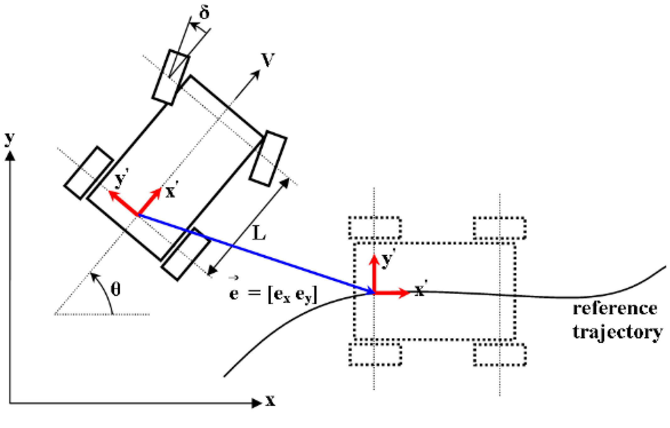
Consider the four-wheeled autonomous orchard vehicle shown in Figure 1. The vehicle has steering and driving wheels at its front and rear, respectively. The steering angle and longitudinal velocity of the vehicle are presented by δ and V, respectively. The length between the rear and front axles is presented by L. The fixed reference frame used to generate the desired trajectory is shown by the (x-y) coordinate axis. The (x′, y′) coordinate system is placed at the rear-axle-center of the vehicle. The orientation of the vehicle is presented by θ. The difference between the reference and actual trajectory is shown by the error vector (e), whose components are e_x and e_y in the x and y directions, respectively.

The objective of this vehicle is to follow rows of trees. It detects the end of each tree row, and turns around to position itself parallel to the next tree row. This motion plan makes it possible to develop an autonomous system that can be used for cherry orchard operations such as production automation, human worker augmentation, spraying, pruning, etc. Motion planning should be able to provide precise straight and turning motions, effectively detect trees and rows of trees, accurately estimate the start and end positions of each row, and produce smooth/reliable control signals for steering and driving systems of the orchard vehicle. In order to develop an autonomous system that can meet these expectations, the following key steps were taken into consideration:

Trees were detected using the data from a laser scanning range finder.

The rows of trees were created by adapting the procedure constructed based on the Hough transform method.

A simple methodology was built to recognize the start and end positions of each row.

In order to achieve turning from one row to another, a turning geometry called knot-like turning was used.

The desired trajectory tracking was achieved using a control strategy which was developed by following the principles of the “smooth time-varying feedback control” method.

In the literature, different kinds of generation methods for reference trajectory for straight and turning motions have been used. Many control strategies have also been proposed to track a reference trajectory. In this study, the main objective was to use a simple modeling structure to generate the desired trajectories for straight motion and turning. Turning geometry was effectively used when there was not enough space for turning operation. Moreover, the trajectory tracking controller was easily modeled and adapted into the overall system model. The trees and rows of trees were estimated with precision. Lastly, the overall mathematical structures created for trajectory generation, estimation and control purposes were adapted into real systems.

2.2. Reference Trajectory Generation

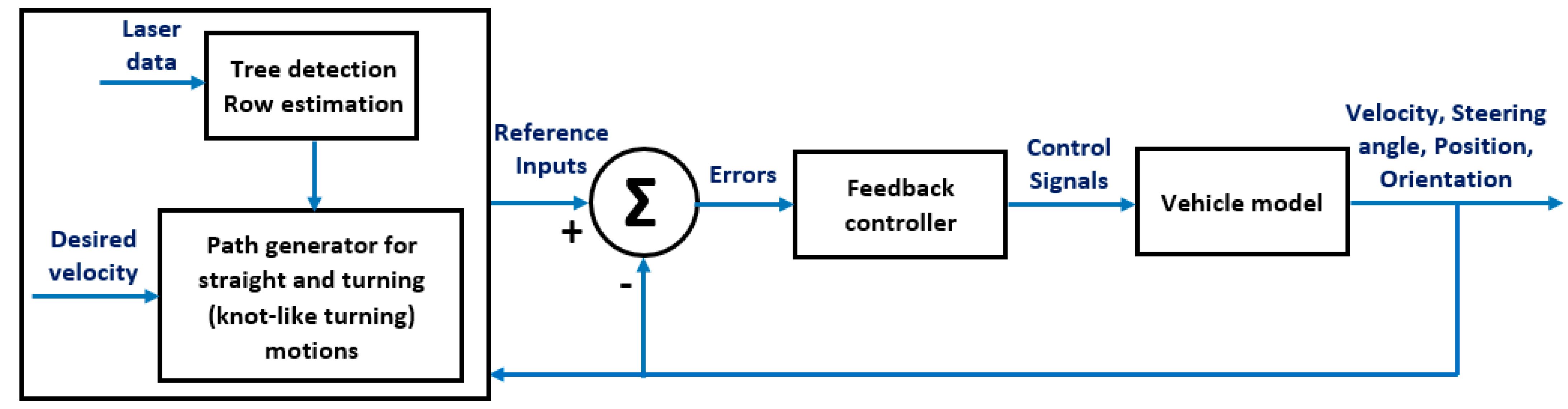
A closed-loop control system block diagram is given in Figure 2 to show the details of the proposed system, which includes reference trajectory generation, knot-like turning, tree detection, row estimation and trajectory tracking control. A reference input block is also shown in this block diagram. The block obtains the data from the laser scanner sensor, and detects trees and estimates the row of trees. It is also responsible for generating the reference trajectory. The control system block diagram was used to develop the simulation environment for observing the performance of the detection of trees and estimation of the rows of trees, desired trajectory generation, turning between rows and generation of control signals.

A car-like robot model can be adapted to the system shown in Figure 1. In this model, the front wheels are steerable, whereas the rear wheels are actuated. A car-like robot model [1,6,22] is constructed in Equations (1)–(4). This basic model and basic trajectory generation structure (Equations (1)–(9)) are preferred in autonomous vehicle applications, since their adaptation, performance and use in real-time performance meet the expectations. The desired velocities of the vehicle in the x (${\dot{\mathrm{x}}}_{\mathrm{d}}$) and y (${\dot{\mathrm{y}}}_{\mathrm{d}}$) directions are given in Equations (1) and (2), respectively. The desired orientation of the vehicle is described by θ_d. Note that subscript “d” represents the desired value. The desired value of the longitudinal velocity is shown by V_d1. The angular velocity is specified by (${\dot{\mathsf{\theta }}}_{\mathrm{d}}$) and given in Equation (3). The steering angle speed given in Equation (4) is illustrated by (${\dot{\mathsf{\delta }}}_{\mathrm{d}}$).

$${\dot{\mathrm{x}}}_{\mathrm{d}}=\cos \left({\mathsf{\theta }}_{\mathrm{d}}\right){\mathrm{V}}_{\mathrm{d}1}$$

(1)

$${\dot{\mathrm{y}}}_{\mathrm{d}}=\sin \left({\mathsf{\theta }}_{\mathrm{d}}\right){\mathrm{V}}_{\mathrm{d}1}$$

(2)

$${\dot{\mathsf{\theta }}}_{\mathrm{d}}=\tan \left({\mathsf{\delta }}_{\mathrm{d}}\right)\left({\mathrm{V}}_{\mathrm{d}1}/\mathrm{L}\right)$$

(3)

The reference speed of the steering angle change can be defined as follows:

$${\dot{\mathsf{\delta }}}_{\mathrm{d}}={\mathrm{V}}_{\mathrm{d}2}$$

(4)

Once the desired velocities in x and y directions are defined (Equations (1) and (2)), the desired forward velocity (longitudinal velocity) of the vehicle can be obtained as follows. Note that the sign of ± indicates the forward and backward motion of the vehicle.

$${\mathrm{V}}_{\mathrm{d}1}=\mp \sqrt{{\dot{\mathrm{x}}}_{\mathrm{d}}{}^2+{\dot{\mathrm{y}}}_{\mathrm{d}}{}^2}$$

(5)

Combining the Equations (1) and (2), the desired orientation of the vehicle can be obtained as given in Equation (6). Note that the atan₂(y,x) solution procedure is used because it is similar to the solution of atan(y/x), except that the signs of the components of (y,x) are used to determine the quadrant of the result.

$${\mathsf{\theta }}_{\mathrm{d}}={\mathrm{atan}}_2\left(\frac{{\dot{\mathrm{y}}}_{\mathrm{d}}}{{\mathrm{V}}_{\mathrm{d}1}},\frac{{\dot{\mathrm{x}}}_{\mathrm{d}}}{{\mathrm{V}}_{\mathrm{d}1}}\right)$$

(6)

The reference angular velocity of the vehicle can also be derived by differentiating Equation (6):

$${\dot{\mathsf{\theta }}}_{\mathrm{d}}=\frac{{\ddot{\mathrm{y}}}_{\mathrm{d}}{\dot{\mathrm{x}}}_{\mathrm{d}}-{\ddot{\mathrm{x}}}_{\mathrm{d}}{\dot{\mathrm{y}}}_{\mathrm{d}}}{{\mathrm{V}}_{\mathrm{d}1}{}^2}$$

(7)

When the desired trajectory is defined, the desired steering angle can also be built as:

$${\mathsf{\delta }}_{\mathrm{d}}=\mathrm{atan}\left(\frac{\mathrm{L}\left({\ddot{\mathrm{y}}}_{\mathrm{d}}{\dot{\mathrm{x}}}_{\mathrm{d}}-{\ddot{\mathrm{x}}}_{\mathrm{d}}{\dot{\mathrm{y}}}_{\mathrm{d}}\right)}{{\mathrm{V}}_{\mathrm{d}1}{}^3}\right)$$

(8)

Finally, the desired steering angle speed can be derived as shown below:

$${\dot{\mathsf{\delta }}}_{\mathrm{d}}={\mathrm{V}}_{\mathrm{d}2}=\frac{\mathrm{L}\left({\stackrel{⃛}{\mathrm{y}}}_{\mathrm{d}}{\dot{\mathrm{x}}}_{\mathrm{d}}-{\stackrel{⃛}{\mathrm{x}}}_{\mathrm{d}}{\dot{\mathrm{y}}}_{\mathrm{d}}\right){\mathrm{V}}_{\mathrm{d}1}{}^3-3{\mathrm{LV}}_{\mathrm{d}1}\left({\ddot{\mathrm{y}}}_{\mathrm{d}}{\dot{\mathrm{x}}}_{\mathrm{d}}-{\ddot{\mathrm{x}}}_{\mathrm{d}}{\dot{\mathrm{y}}}_{\mathrm{d}}\right)\left({\ddot{\mathrm{x}}}_{\mathrm{d}}{\dot{\mathrm{x}}}_{\mathrm{d}}+{\ddot{\mathrm{y}}}_{\mathrm{d}}{\dot{\mathrm{y}}}_{\mathrm{d}}\right)}{{\mathrm{V}}_{\mathrm{d}1}{}^6+{\mathrm{L}}^2{\left({\ddot{\mathrm{y}}}_{\mathrm{d}}{\dot{\mathrm{x}}}_{\mathrm{d}}-{\ddot{\mathrm{x}}}_{\mathrm{d}}{\dot{\mathrm{y}}}_{\mathrm{d}}\right)}^2}$$

(9)

2.3. Controller Design

The control signals required for actuating the steering and driving systems of the vehicle are generated by following the principles of the smooth time-varying feedback control strategy [1,4,5,6,22,23]. The control method uses the chained system rule to decompose the solution techniques in two design stages. In the first design stage of the controller, one control input is provided such that some design requirements are satisfied. Then, the other controller is constructed in order to ensure the stability of (n − 1) dimensional system state. In the second stage, the objective is to guarantee the convergence of the system variables. In this design stage, the overall closed-loop control system stability should be achieved. To set up a new system state, the following form is considered:

$$\tilde{\mathrm{X}}=\left({\tilde{\mathrm{X}}}_1,{\tilde{\mathrm{X}}}_2,\dots \; \dots ,{\tilde{\mathrm{X}}}_{\mathrm{n}-1},{\tilde{\mathrm{X}}}_{\mathrm{n}}\right)=\left({\mathrm{x}}_1,{\mathrm{x}}_2,\dots \; \dots ,{\mathrm{x}}_{\mathrm{n}}\right)$$

(10)

The chain rules are used for reference trajectory generation and controller design. They are also used to define new states and a reference system. The chained form for the system introduced here can be constructed in the following form:

$$\begin{array}{l}\begin{array}{l}{\dot{\tilde{\mathrm{X}}}}_1={\mathrm{V}}_1\hfill \\ {\dot{\tilde{\mathrm{X}}}}_2={\tilde{\mathrm{X}}}_3{\mathrm{V}}_1\hfill \\ {\dot{\tilde{\mathrm{X}}}}_3={\tilde{\mathrm{X}}}_4{\mathrm{V}}_1\hfill \\ \cdots \hfill \\ \cdots \hfill \\ \cdots \hfill \\ {\dot{\tilde{\mathrm{X}}}}_{\mathrm{n}-1}={\tilde{\mathrm{X}}}_{\mathrm{n}}{\mathrm{V}}_1\hfill \\ {\dot{\tilde{\mathrm{X}}}}_{\mathrm{n}}={\mathrm{V}}_2\hfill \end{array}\hfill \end{array}$$

(11)

where V₁ and V₂ indicate the longitudinal and steering angle velocities, respectively. Adapting the (2, 4) chained form to develop the feedback controllers for the steering and driving systems gives the following new state variables (${\tilde{\mathrm{X}}}_{\mathrm{i}}$, i = 1,…,4). Note that the details are omitted here for clarity. Interested readers may refer to the studies [1,4,5,6,22,23] for details.

$$\begin{array}{l}{\tilde{\mathrm{X}}}_1={\mathrm{x}}_{\mathrm{d}}-\mathrm{x}={\mathrm{x}}_{\mathrm{e}}\hfill \\ {\tilde{\mathrm{X}}}_2={\mathrm{y}}_{\mathrm{d}}-\mathrm{y}={\mathrm{y}}_{\mathrm{e}}\hfill \\ {\tilde{\mathrm{X}}}_3=\tan ({\mathsf{\theta }}_{\mathrm{d}}-\mathsf{\theta })=\tan ({\mathsf{\theta }}_{\mathrm{e}})\hfill \\ {\tilde{\mathrm{X}}}_4=\left(\tan \left(\mathsf{\delta }\right)-\cos \left({\mathsf{\theta }}_{\mathrm{d}}-\mathsf{\theta }\right)\tan \left({\mathsf{\delta }}_{\mathrm{d}}\right)\right)\left(\frac{1}{\left(\mathrm{L}\cos {\left({\mathsf{\theta }}_{\mathrm{d}}-\mathsf{\theta }\right)}^3\right)}\right)+{\mathrm{k}}_2\left({\mathrm{y}}_{\mathrm{d}}-\mathrm{y}\right)\hfill \end{array}$$

(12)

where x_d and y_d show the x–y components of the desired trajectory. ϴ_d and δ_d represent the desired orientation angle and steering angle of the vehicle moving on the desired trajectory, respectively. Tracking errors in the x and y directions are given by x_e and y_e, respectively. The orientation error is shown by ϴ_e. k₂ is the control parameter which is to be defined according to the system specifications. The time derivatives of the new state variables (${\dot{\tilde{\mathrm{X}}}}_{\mathrm{i}}$, i = 1,..,4) are derived in the following form:

$$\begin{array}{l}{\dot{\tilde{\mathrm{X}}}}_1=\left({\tilde{\mathrm{X}}}_{\mathrm{d}}/\mathrm{L}\right)\tan \left({\mathsf{\delta }}_{\mathrm{d}}\right){\tilde{\mathrm{X}}}_2+{\mathrm{V}}_1\hfill \\ {\dot{\tilde{\mathrm{X}}}}_2=\left(-{\tilde{\mathrm{X}}}_{\mathrm{d}}/\mathrm{L}\right)\tan \left({\mathsf{\delta }}_{\mathrm{d}}\right){\tilde{\mathrm{X}}}_1+{\tilde{\mathrm{X}}}_{\mathrm{d}}{\tilde{\mathrm{X}}}_3+{\mathrm{V}}_1{\tilde{\mathrm{X}}}_3\hfill \\ {\dot{\tilde{\mathrm{X}}}}_3=\left(-{\mathrm{k}}_2{\tilde{\mathrm{X}}}_{\mathrm{d}}{\tilde{\mathrm{X}}}_2\right)+{\tilde{\mathrm{X}}}_{\mathrm{d}}{\tilde{\mathrm{X}}}_4+{\mathrm{V}}_1\left({\tilde{\mathrm{X}}}_4-{\mathrm{k}}_2{\tilde{\mathrm{X}}}_2+\left(1+{\tilde{\mathrm{X}}}_3{}^2\right)\tan \left({\mathsf{\delta }}_{\mathrm{d}}\right)/\mathrm{L}\right)\hfill \\ {\dot{\tilde{\mathrm{X}}}}_4={\mathrm{V}}_2\hfill \end{array}$$

(13)

The feedback controllers, which are specified by longitudinal velocity (V₁) and steering angle speed (V₂), can be described in the following form:

$$\begin{array}{l}{\mathrm{V}}_1=-{\mathrm{k}}_1\left|{\mathrm{U}}_{\mathrm{d}1}\right|\left({\tilde{\mathrm{X}}}_1+\left(\frac{{\tilde{\mathrm{X}}}_2{\tilde{\mathrm{X}}}_4}{{\mathrm{k}}_2}+\frac{{\tilde{\mathrm{X}}}_2}{{\mathrm{k}}_2{\tilde{\mathrm{X}}}_3{}^2}\right)\tan \left({\mathsf{\delta }}_{\mathrm{d}}\right)/\mathrm{L}\right)\hfill \\ {\mathrm{V}}_2=-{\mathrm{k}}_3\left|{\mathrm{U}}_{\mathrm{d}1}\right|\left({\tilde{\mathrm{X}}}_3{\tilde{\mathrm{X}}}_4-{\mathrm{k}}_4{\tilde{\mathrm{X}}}_4\left|{\mathrm{U}}_{\mathrm{d}1}\right|\right)\hfill \end{array}$$

(14)

where k₁, k₃ and k₄ are the other control parameters which are to be defined. In Equation (14), the values of the desired (reference) controller indicated by U_d1 and U_d2 are specified as:

$$\begin{array}{l}{\mathrm{U}}_{\mathrm{d}1}={\dot{\mathrm{x}}}_{\mathrm{d}}\hfill \\ {\mathrm{U}}_{\mathrm{d}2}=\left({\stackrel{⃛}{\mathrm{y}}}_{\mathrm{d}}{\dot{\mathrm{x}}}_{\mathrm{d}}{}^2-{\stackrel{⃛}{\mathrm{x}}}_{\mathrm{d}}{\dot{\mathrm{y}}}_{\mathrm{d}}{\dot{\mathrm{x}}}_{\mathrm{d}}-3{\ddot{\mathrm{y}}}_{\mathrm{d}}{\dot{\mathrm{x}}}_{\mathrm{d}}{\ddot{\mathrm{x}}}_{\mathrm{d}}+3{\dot{\mathrm{y}}}_{\mathrm{d}}{\ddot{\mathrm{x}}}_{\mathrm{d}}{}^2\right)\left(1/{\dot{\mathrm{x}}}_{\mathrm{d}}{}^4\right)\hfill \end{array}$$

(15)

where longitudinal and lateral velocities, accelerations, and jerks in the x and y directions are specified by $\left({\dot{\mathrm{x}}}_{\mathrm{d}},{\dot{\mathrm{y}}}_{\mathrm{d}}\right), \left({\ddot{\mathrm{x}}}_{\mathrm{d}},{\ddot{\mathrm{y}}}_{\mathrm{d}}\right), \left({\stackrel{⃛}{\mathrm{x}}}_{\mathrm{d}},{\stackrel{⃛}{\mathrm{y}}}_{\mathrm{d}}\right)$, respectively.

2.4. Turning Geometry

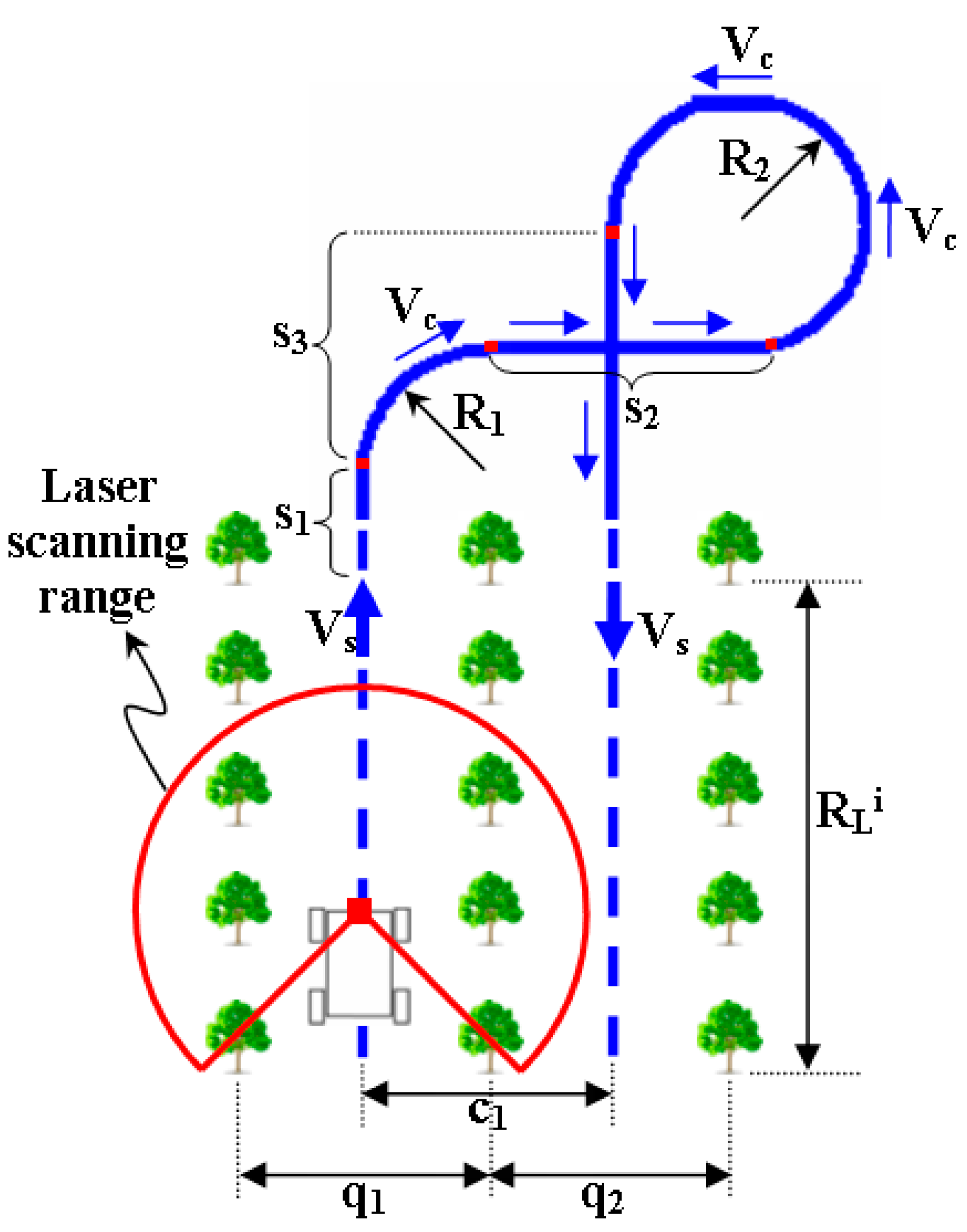
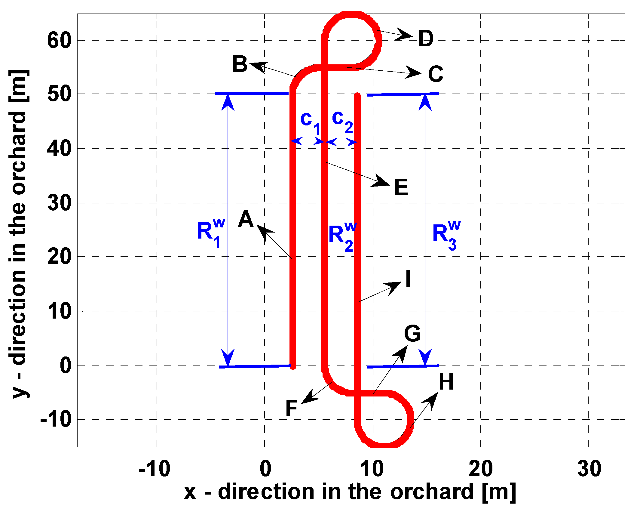
The vehicle that follows the center line of two consecutive rows must perform a turning when it comes to the end of a row. Different types of turning strategies, such as clothoid turning [24] and bulb-shape turning [25], have been developed. In both turning strategies, the turning geometry should be described in an equation form. This form also requires some computational effort, which may be a problem in real-time operations. In the case that the turning space is not big enough for clothoid, bulb-shape, U-shape or K-shape turnings, the turning strategy introduced in this study can also be used. In this study, a new kind of turning methodology (called knot-like turning) was proposed, as presented in Figure 3. The advantage of this turning strategy is that it can be described by the combination of simple straight lines and circles. Therefore, a complete environment model is not needed. The vehicle is located at the beginning of the first row, and the rest is completed via the combination of lines and circles, which creates the reference path. The use of this simple combination makes it possible arrange the straight line and circle parameters (s₁, s₂, s₃, R₁, R₂, V_s, V_c) according to the row width information (c₁) in an easy way (i.e., use of a look-up table). Another advantage of adapting knot-like turning in an orchard application is that there is enough time and distance when the last turn (of which radius is shown by R₂) is completed. Before entering the next row, the (autonomous) vehicle has time to check its surroundings, whether it goes through the right row and whether the motion is safe (i.e., there is no possibility to crash into trees). Note that the cherry orchard where the laser sensor data were collected was professionally organized. The plantation geometries of the rows of trees, the row widths and the spare spaces for turning operations were well planned. Therefore, while the modeling structure was constructed, it was assumed that there would be always enough spare space for turning.

In Figure 3, row centers and turnings are indicated by dashed and solid lines, respectively. The velocities of the vehicle during straight and turning motions are defined by V_s and V_c, respectively. The vehicle considered in this study was equipped with a laser scanner rangefinder placed at the front-mid-center. The row widths (q_i) and row lengths (R_Lⁱ) were obtained using the information from this sensor. The turning geometry was generated according to the information of the available turning space. Considering the case shown in Figure 3, the available turning space should be equal to or bigger than the value of (s₁ + s₃ + R₂). The turning methodology introduced here only needs the information of the row widths. Then, the turning algorithm can calculate the radiuses of R₁ and R₂, and the lengths of s₁, s₃ and s₂.

2.5. Scanning of Trees of a Cherry Orchard Using a Laser Scanner Rangefinder

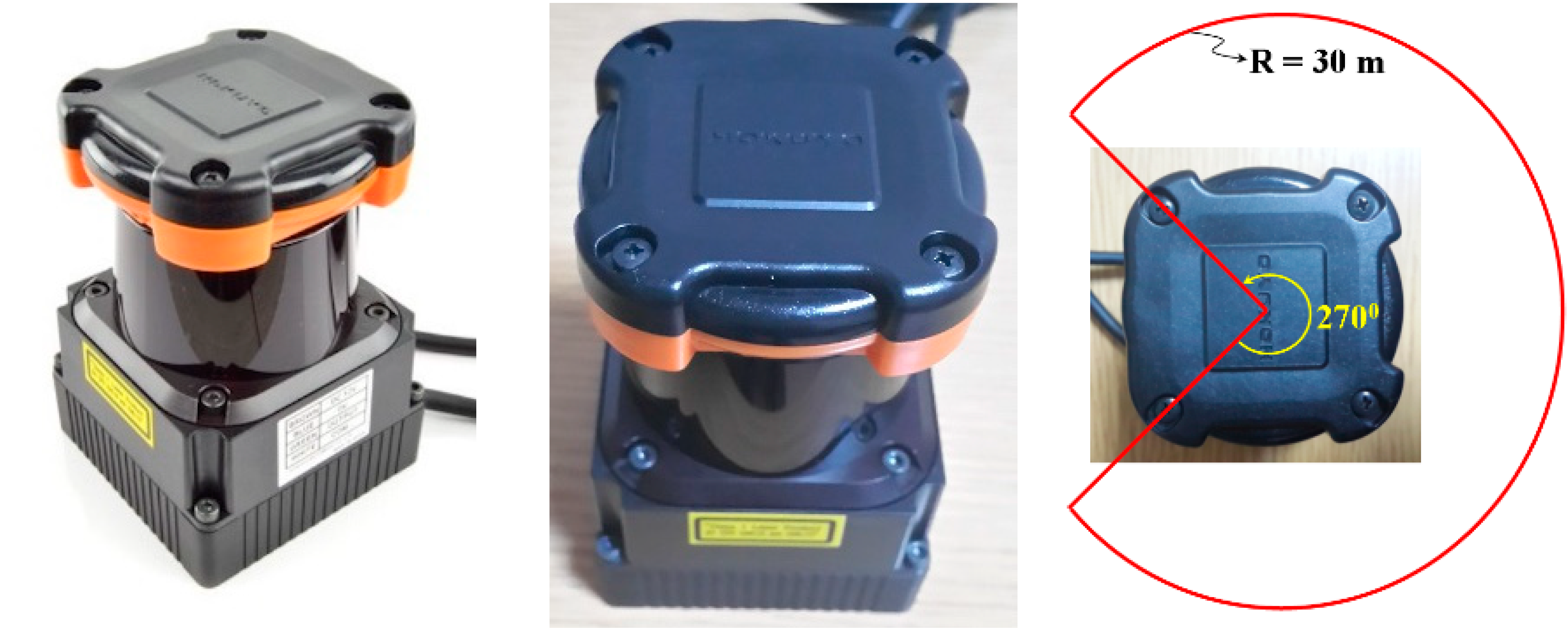
Trees and rows of trees of one of the Napoleon cherry orchards located in Mihaliccik region of Turkey (Eskisehir) were scanned using the laser scanner rangefinder shown in Figure 4. A branch with the Napoleon cherries is shown in Figure 5. The laser scanner was placed at the center of the rows, and the scanning data were recorded.

The laser scanner (Figure 4), Hokuyo UTM-30LX, has a scanning capability of up to 30 m. This property is indicated in the right image of Figure 4. The scanning area is shown by the red circle, and maximum scan range is indicated by the radius information (R = 30 m). The scanning angle range is also presented by the yellow circular arrow, which shows the scanning range of 270°. The angular resolution of the laser scanner is 0.25°, which means a full scan provides 1080 distance information. The power requirement for this sensor is 12 VDC with a maximum of 1 A current. The sensor sends a data package, which should be decoded using a computer or a microprocessor. In this study, the decoding process was achieved in the Matlab/Simulink environment using a Real-Time Workshop toolbox. The sensor data were handled in every 10 Hz, which also determined the sampling frequency of the control action (the time interval between two control actions was set to 0.1 s).

2.6. Detection of Trees

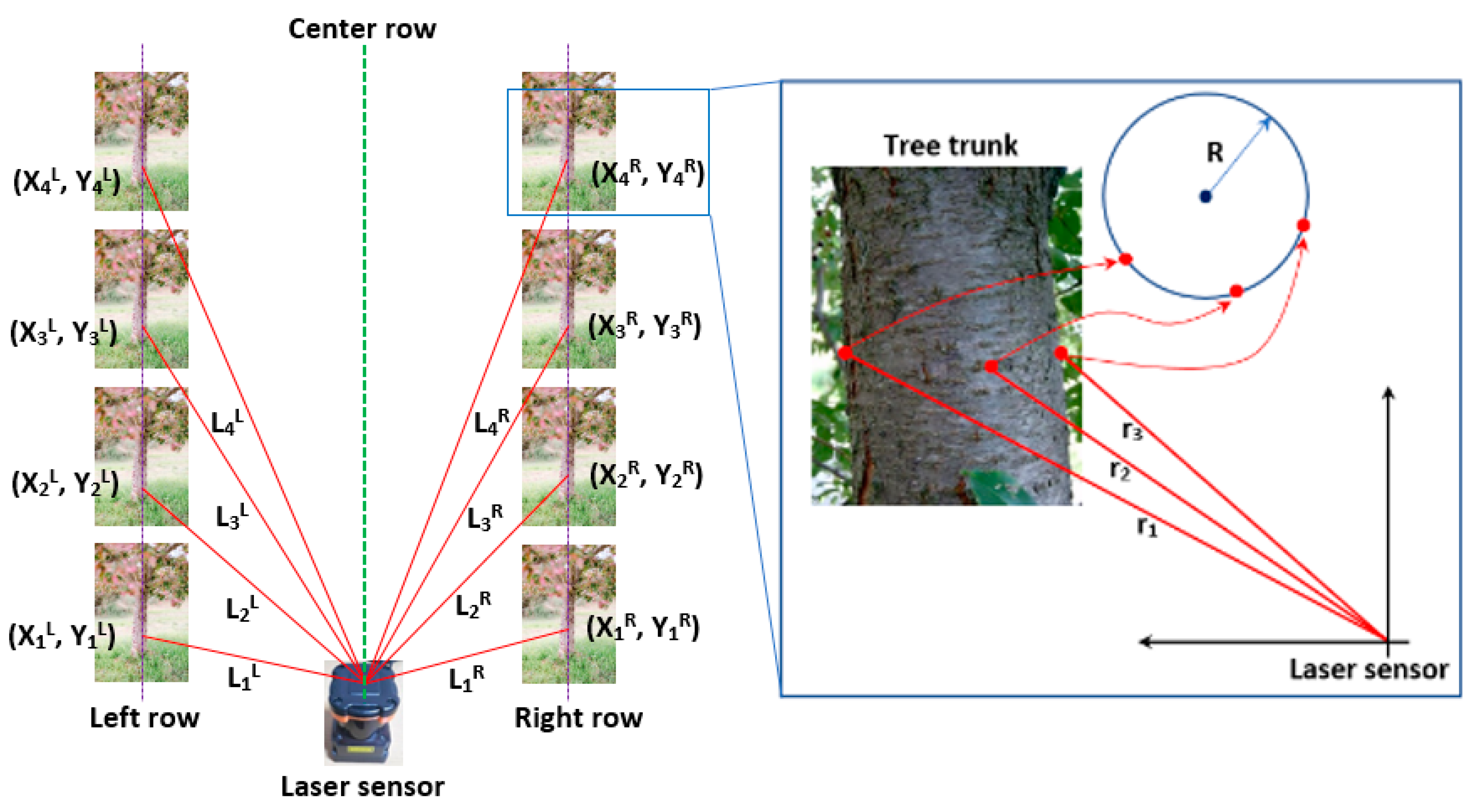
In this study, the aim was to keep the vehicle in the row center while it was in motion. In order to achieve this objective, the right and left rows of trees should be recognized so that the error between the vehicle and the row center can be measured. The accurate line equations for the right and left rows can be created as long as the trees are detected with minimum detection errors. The principles of the detection of trees and estimation of rows of trees are depicted in Figure 6. The test environment is presented with two rows of trees in this figure. The distance between two tree rows was approximately 4 m, and the length of each row was about 20 m. The laser scanner scanned its surrounding, and each tree was detected using at least three laser scan measurements, as shown in the zoomed view in Figure 6. In Figure 6, the distances between the laser scanner and the detected trees is shown by L_i^R and L_i^L for the trees at the right and left of the vehicle (i = 1, 2, 3, 4, ….), respectively. Note that only four of detected trees on each side are shown in this representation. The tree locations shown by (X_i^R, Y_i^R) and (X_i^L, Y_i^L) were also determined using the distance and scan angle information.

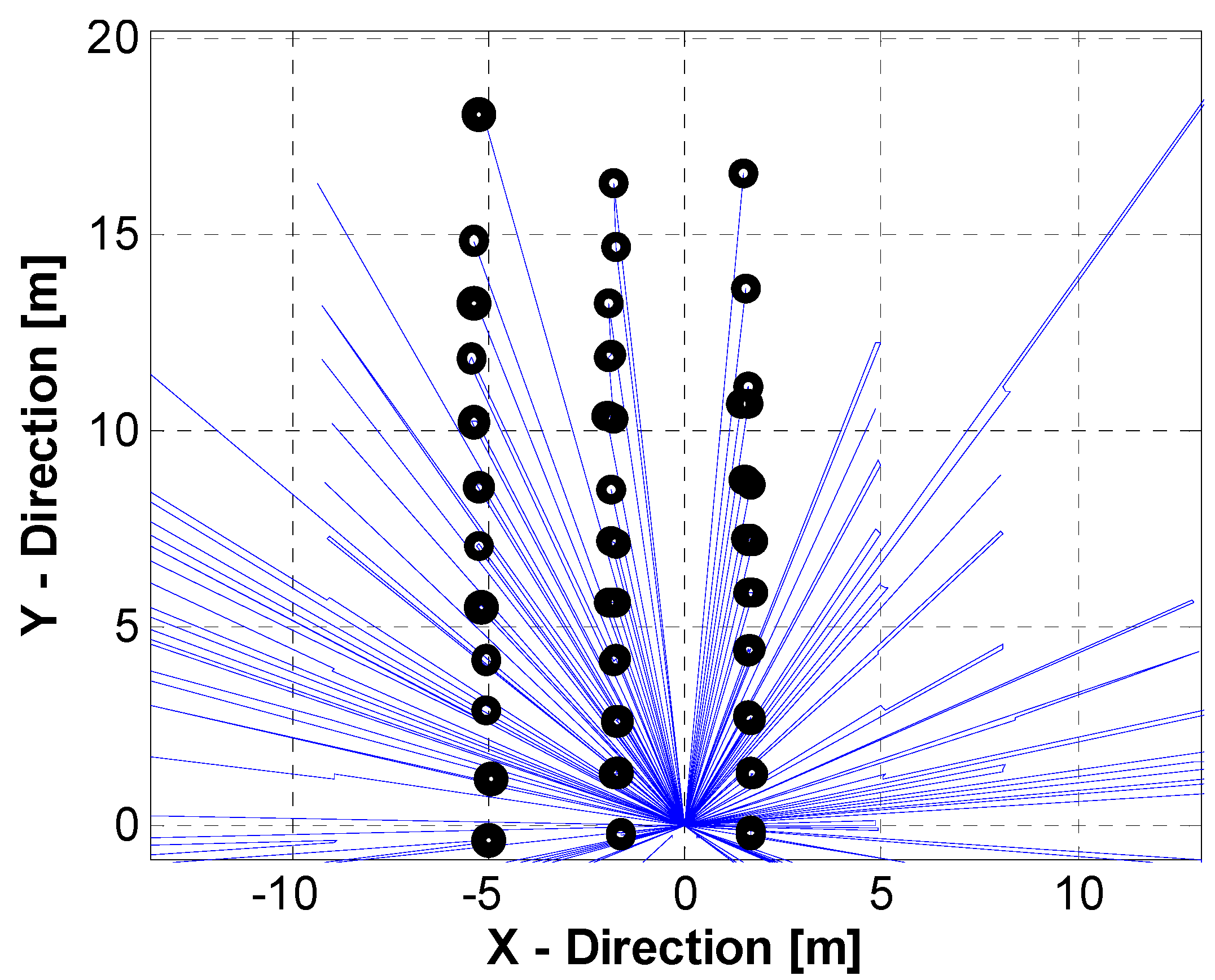
In order to test the tree detection procedure mentioned above, the recorded laser scanner data were moved to the simulation environment. The developed algorithm detected the trees, as exhibited in Figure 7 (detected trees are indicated by black-colored circles). As seen in the figure, the detected trees formed three neighboring rows of trees.

2.7. The Use of Hough Transform Method for Row Estimation

Trees detected using the methodology described above were used to estimate the rows of trees. (Note that in this study, it was assumed that two adjacent tree rows were parallel, since the trees in the cherry orchard where the laser data were collected were professionally planted to create straight rows of trees.) The tree lines shown by “Left Row” and “Right Row” in Figure 6 were created using the algorithm, which was developed by adapting the Hough transform method. The principles of Hough transform can be given as follows: A line in a 2D plane is described using an equation which has a form of y = mx+k, where m and k are slope and intercept, respectively. When there are many points (x_i, y_i) in a data set, y_i = m(x_i) + k is constructed by a sufficient number of points. As long as the points (x_i, y_i) lie on the same line, the values of m and k should be unique. On the other hand, the polar coordinate system guarantees that the line equation can be represented via r = x cosθ + y sinθ. 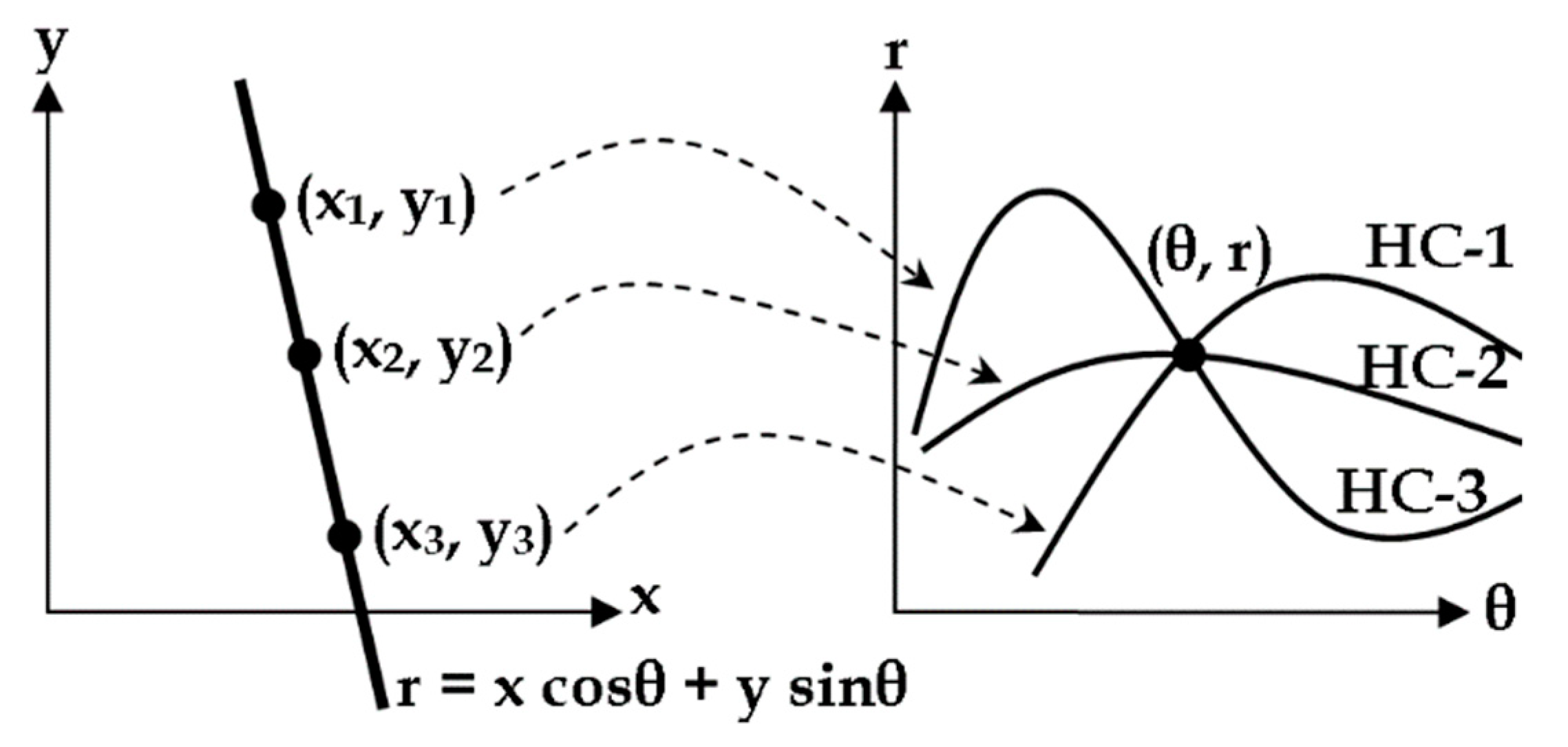This representation determines the unique locations of (r, θ) for the points (x_i, y_i), which show lines on a curve in the Hough space, known as Hough transform. The principles of Hough transform are represented in Figure 8 using a simple example including only three points. In this example, the Hough transform takes the points (x₁, y₁), (x₂, y₂) and (x₃, y₃), and maps them into the Hough curves (HC) at the point (θ, r) of the Hough space. The points (x_i, y_i) and (θ, r) are illustrated in the left and right images of Figure 8, respectively.

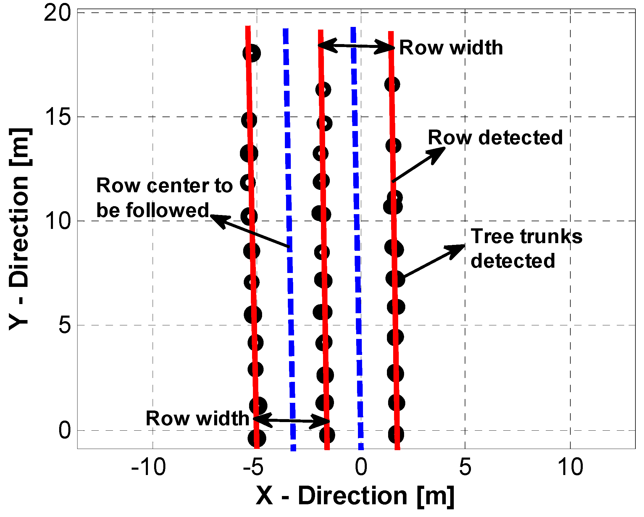
When the Hough transform method was adapted into the system introduced here (detected trees shown in Figure 7), the rows of trees were estimated, as illustrated in Figure 9. In the estimation process, Hough transform generates a line which connects the number of trees in a row of trees. This estimation is performed for both the right and left rows of trees. This process generates the line equations r_j = x_j cos(θ_j) + y_j sin(θ_j) (where j indicates right and left) for the right and left rows of trees. The position information of the trees (x_i, y_i), i = 1, 2, 3,…, n are mapped into Hough space and create n Hough curves to estimate the unique values of ϴ and r. In Figure 9, the red-colored solid lines show the estimated rows of trees. The row centers, considered as the straight parts of the reference trajectory, are indicated via blue-colored dashed lines. The approximate row width used to generate a reference turning geometry (Figure 3) was also obtained by this estimation.

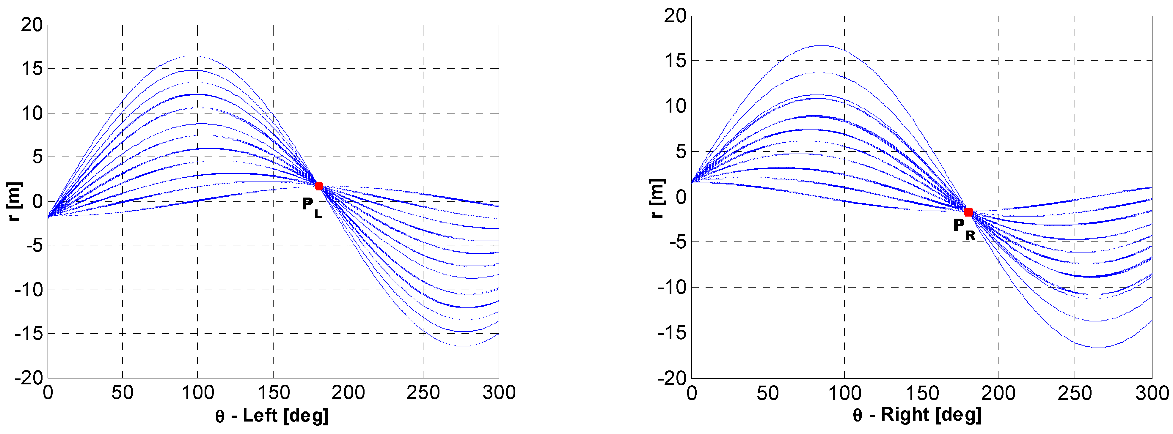
Hough curves mapped into Hough space are also illustrated for the row center lines (left and right dashed lines in Figure 9) in Figure 10.

3. Results and Discussion

As described above, the laser scanner data were used for detecting each tree in the cherry orchard. Then, the information of the detected trees was transferred to the algorithm developed for estimating the rows of trees. These two steps provide the necessary data used to generate the desired (reference) trajectory. In order to test the trajectory tracking performance and accuracy of the developed system, a simulation environment was created in Matlab. The reference trajectory was given to this environment as the input. In addition, the errors that occurred between the input and output trajectories were observed. Furthermore, the behaviors of the steering and driving controllers were also tested. The simulation environment also provided the opportunity to test the performance of the proposed knot-like turning method. The results obtained in the simulation studies make it possible to test the developed system before adapting it into a real system.

In the simulation studies, the row centers estimated using Hough transform (Figure 9) were used to create the straight parts of the desired trajectory. The turning geometry introduced in Figure 3 was adapted to the system to build the turning parts of the desired trajectory. The desired trajectory and tracking results are presented in Figure 11, Figure 12 and Figure 13. The straight and curved parts of the motion are specified by the letters A–H (Figure 11) to present the results in detail. Note that in order to test the performance of the feedback controller introduced in Section 2.3, Gaussian white noise was added to the straight parts of the desired trajectory (specified by the letters A, C, E, G and I).

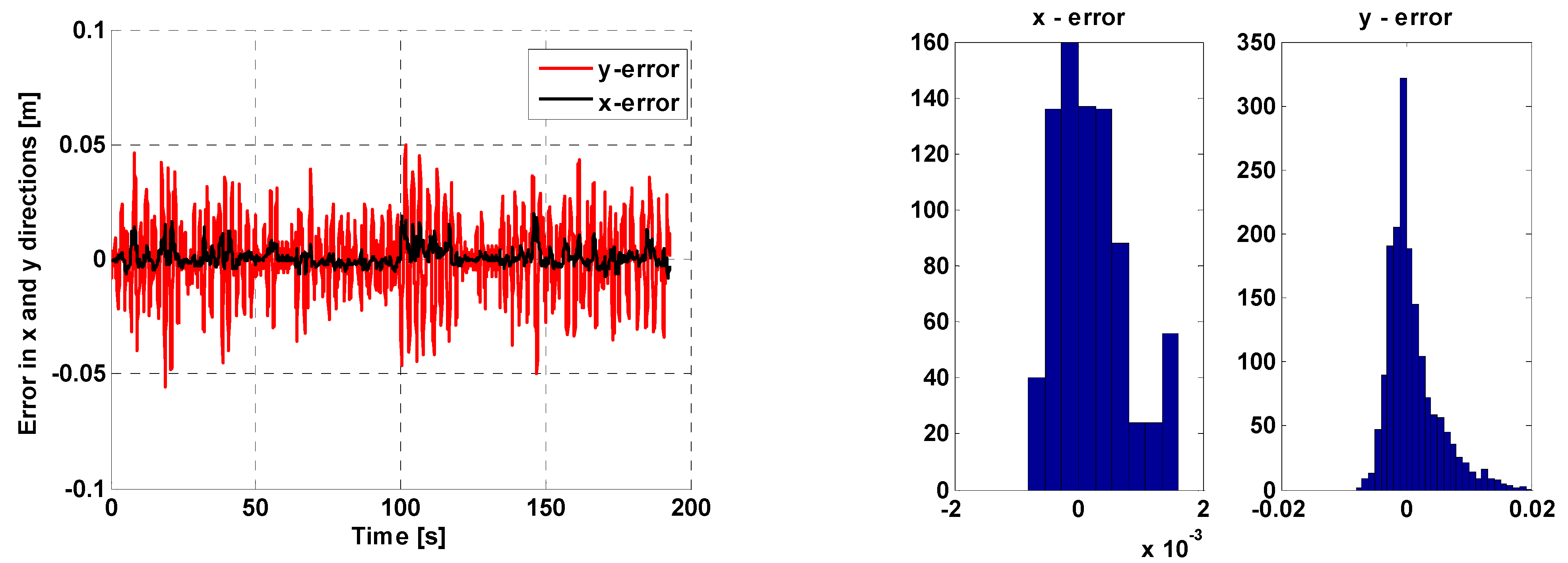
Errors obtained in x and y directions are given in the left image of Figure 12 by the black and red solid lines, respectively.

The histogram plots of x and y errors are also given in the right image of Figure 12. These results indicate that the errors occurring in the x direction were accumulated between −0.001 and 0.002 m, whereas those in the y direction were observed in the region between the −0.01 and 0.02 m band.

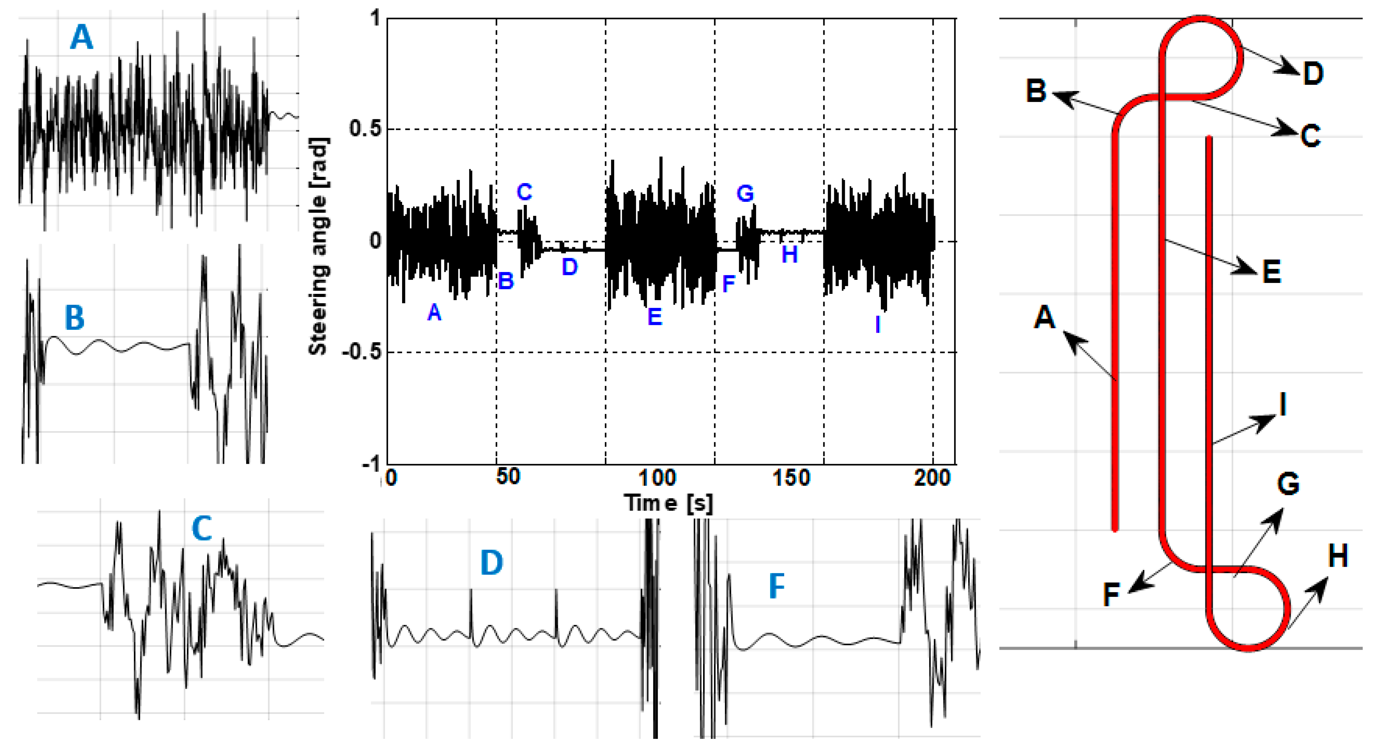
Figure 13 exhibits the control signals generated for the steering angle. In order to show the variations in steering angle, a couple of zoomed-in-views are also presented. The locations of the specified motions are also shown in the right image in Figure 13. The letters shown in this figure specify the straight and turning parts of the reference trajectory (see Figure 11). Despite the additive Gaussian white noise in the straight parts of the reference trajectory, the controller was able to generate the required steering angle comments to achieve trajectory tracking with minimal tracking errors.

4. Conclusions

The smooth time-varying feedback control method is used for autonomous vehicle applications. It generates the necessary commands to follow a desired trajectory. In this study, this procedure was adapted to an autonomous orchard vehicle task. The vehicle’s motion and reference trajectory were developed by following the principles of a car-like robot model. The modeling structure was integrated with the feedback control strategy. A new type of turning strategy for turning from one row to another was proposed. An algorithm was developed to detect trees and estimate rows of trees. An estimation procedure was constructed based on the Hough transform method. A simulation environment was created to determine the performance of the proposed system. The trees and rows of trees of a cherry orchard were scanned using a laser scanner rangefinder. The scanned data were then transferred to the simulation environment to create the desired trajectory, and the simulations were conducted for a trajectory tracking task. The results indicate that the proposed system, including the adaptation of the car-like robot model, desired trajectory generation, turning procedure and smooth time-varying feedback control, could be effectively used for autonomous orchard applications. As a future work, the methodology introduced in this paper will be adapted into a real robot vehicle designed for performing autonomous cherry orchard applications. Conducting real experiments in cherry orchards will make it possible to verify the system presented here.