Soil Particle Modeling and Parameter Calibration Based on Discrete Element Method

Abstract

In order to establish a Discrete Element Method (DEM) model of soil particles, the soil in the laboratory soil bin was used as the research object. The soil texture was determined to be sandy loam by sieving, and the shape of the soil particles was analyzed by an image particle analyzer to establish a geometric model of the soil particles. The Edinburgh Elasto-Plastic Adhesion (EEPA) model was chosen as the contact model for the soil particle simulation analysis, and the accuracy of the model selection was determined by texture tests. The parameters in the contact model played a crucial role in the results of the simulation. Test methods were used to obtain parameters for the soil particles that were easy to measure. For parameters that could not be measured in the contact model, a direct shear test was used as the calibration test, and after screening the sensitive parameters using the PB test, the response surface method was used to calibrate the sensitive parameters. The accuracy of the calibration results was verified by comparing the simulation and test results of the direct shear test under different loadings.

1. Introduction

The DEM is now widely used in the field of agricultural engineering [1,2,3]. During sowing, field management, and harvesting, there is inevitably interaction between soil particles, between soil particles and seeds, and between soil particles and boundaries [4,5,6]. When the DEM is used to analyze the above-mentioned interactions, a DEM model of the soil particles is first established.

Ucgul et al. established a spherical model of soil particles with a radius of 10 mm and analyzed the soil after plough tillage. The results showed that the simulated values of the lateral and forward movement of the surface soil were larger than the measured values, and the simulation of the deep soil agreed well with the test results [7]. Bravo et al. developed a spherical model of soil particles to simulate a soil direct shear test. Particle models with different particle sizes (3–4 mm in the surface layer, 4–6 mm in the middle layer, and 6–8 mm in the bottom layer) were used to fill the soil bin, and soil tillage in hard–dry, soft–wet, and friable states was simulated and analyzed [8]. Our analysis showed that the particles in the soil particle models established by various scholars are large and spherical, which is different from the actual size and shape of soil particles. Therefore, the size and shape of soil particles need to be studied in depth.

The different textures of soil particles require different contact models for simulation analysis. Chen et al. conducted a deep loosening test and simulation on three different soils (coarse sand, loam, and sandy loam) using a parallel bond model (PBM). The simulation and test results for the soil cutting force and soil disturbance characteristics caused by deep loosening were compared and analyzed. The results showed that the relative error was less than 10% in most cases [9]. Xiang et al. used the Hertz–Mindlin with JKR model (JKR model) to analyze clay loam soils in southern China. The parameters of the JKR model were calibrated by angle of repose tests. The accuracy of the DEM model for reflecting the physical and mechanical properties of the soil was verified by comparing the simulation of hole formation with the soil bin test [10]. Our analysis showed that there are a variety of contact models applicable to the simulation of soil particles. However, most scholars do not provide an explanation of why the corresponding contact model was used for the test soil. Therefore, the contact model chosen for the test soil and the accuracy of the model require further analysis and research.

Soil particles have a number of parameters which can play a very significant role in simulation results. Ucgul et al. determined the DEM parameters required to simulate soil tillage processes by means of an angle of repose test and a cone penetration test. The results showed that when the appropriate contact model and parameters were adopted, the DEM could effectively predict the interaction force between non-cohesive soil and tools and simulate the movement of soil particles [7]. Bravo et al. obtained the macroscopic parameter values of soil mechanical properties by a direct shear test. The values of parameters such as the elastic modulus, shear strength, friction coefficient, and cohesion of the soil were obtained by statistical regression equations. The accuracy of the model was also verified by comparing the simulation with test results using a soil bin tillage test [8]. The combinations of parameters measured by the abovementioned scholars without analyzing their sensitivity are not accurate enough and may differ significantly from the actual values. When there are many parameters to be determined, the parameters that need to be calibrated and the calibration methods should be studied in depth.

Based on the abovementioned problems, a geometric model of soil particles was established in this paper after conducting a shape analysis. According to the characteristics of the test soil, the EEPA model was chosen for the contact model. The direct shear test was used as a calibration test, and sensitive parameters were screened by PB tests for unmeasurable simulation parameters. Further the sensitive parameters were calibrated using the response surface method, and the accuracy of the calibrated parameters was verified.

2. Geometric Modeling of Soil Particles

2.1. Soil Particle Size Distribution and Texture

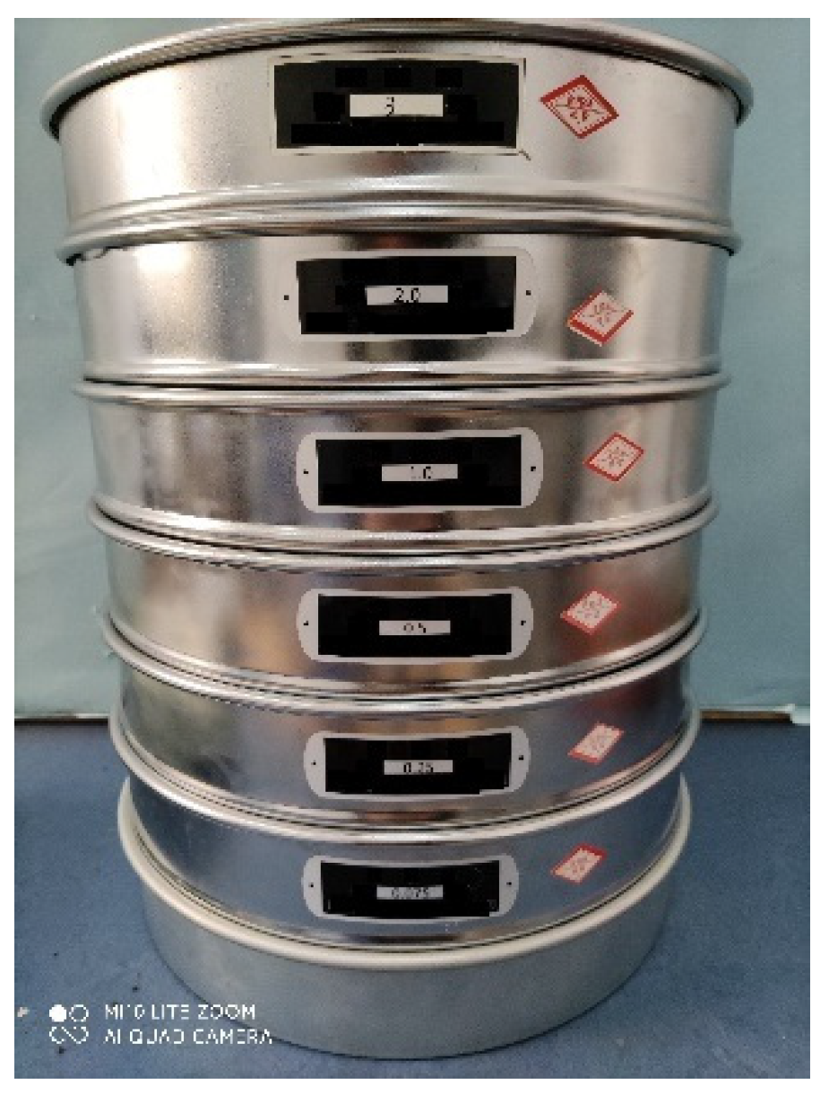
The test soil was sieved through a 3 mm diameter soil sieve. A Chinese standard soil sieve was selected, as shown in Figure 1. The soil was sieved and tested with sieve diameters of 2 mm, 1 mm, 0.5 mm, 0.25 mm, and 0.075 mm, arranged in order from top to bottom, with a collection box at the base.

After sieving, the soil particles were weighed in the different particle size ranges, and three replicate tests were carried out to analyze the test data, as shown in

Table 1. Mass distribution of soil particles in different particle size ranges.

Test Number	Mass of Soil Particles (g)
	2~3 mm	1~2 mm	0.5~1 mm	0.25~0.5 mm	0.075~0.25 mm	0~0.075 mm
1	36.48	31.97	92.59	68.21	45.86	21.48
2	26.44	25.67	95.3	76.43	51.2	21.99
3	35.72	27.51	98.63	70.44	45.3	20.59
Average value	32.88	28.38	95.51	71.69	47.45	21.35
Content percentage (%)	11.06	9.55	32.13	24.12	15.96	7.18

.

The mass percentage of soil particles was 79.39%, 9.55%, and 11.06% for the particle size ranges of 0~1 mm, 1~2 mm, and 2~3 mm, respectively. By comparing the soil texture classification criteria [11], it was clear that the soil type selected for testing was sandy loam.

2.2. Geometric Model of Soil Particles

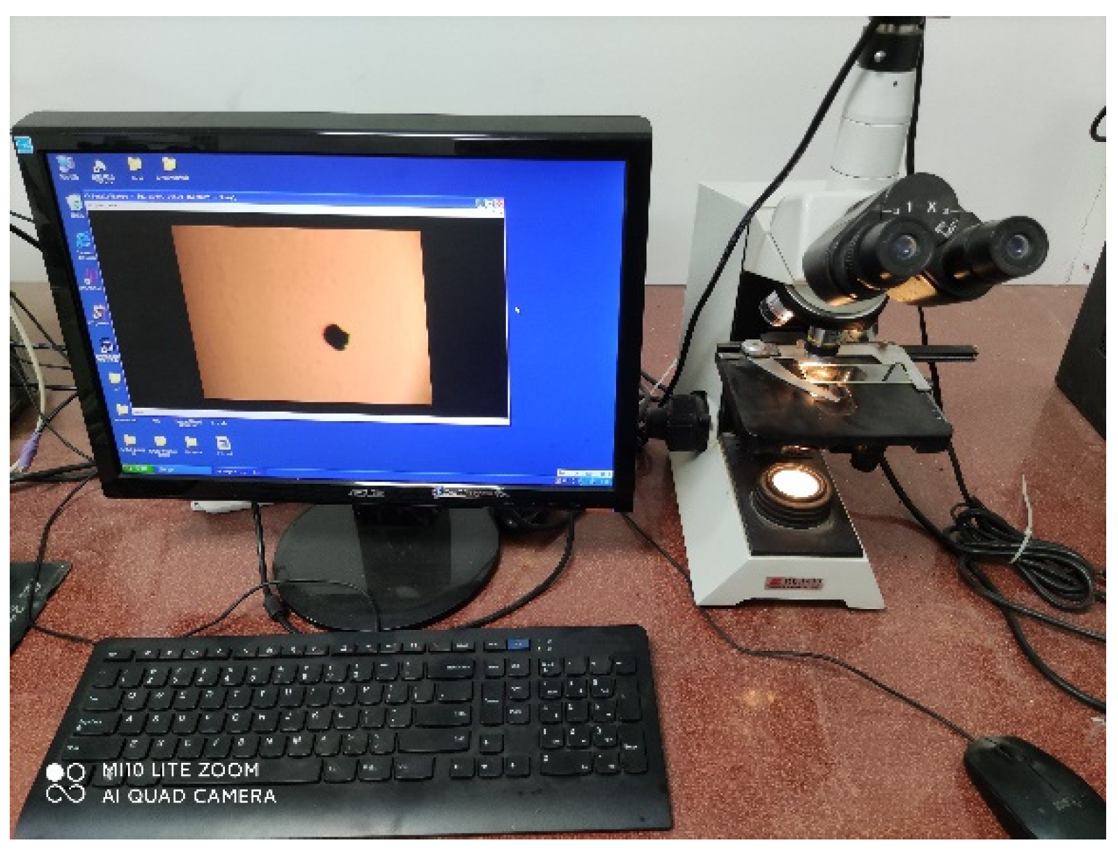
In order to study the shape of the soil particles and facilitate the establishment of their geometric model, the soil particles were scanned and analyzed using an XS-2100 image particle analyzer, as shown in Figure 2.

The test procedure was as follows: soil particles with a particle size range of 0~0.075 mm were placed on a slide of the image particle analyzer. A sample of 30 soil particles was taken, and the shape of each particle was observed on a computer after magnification. Using the same method, enlarged images of soil particles with particle sizes ranging from 0.075 to 0.25 mm, 0.25 to 0.5 mm, and 0.5 to 1 mm were obtained. 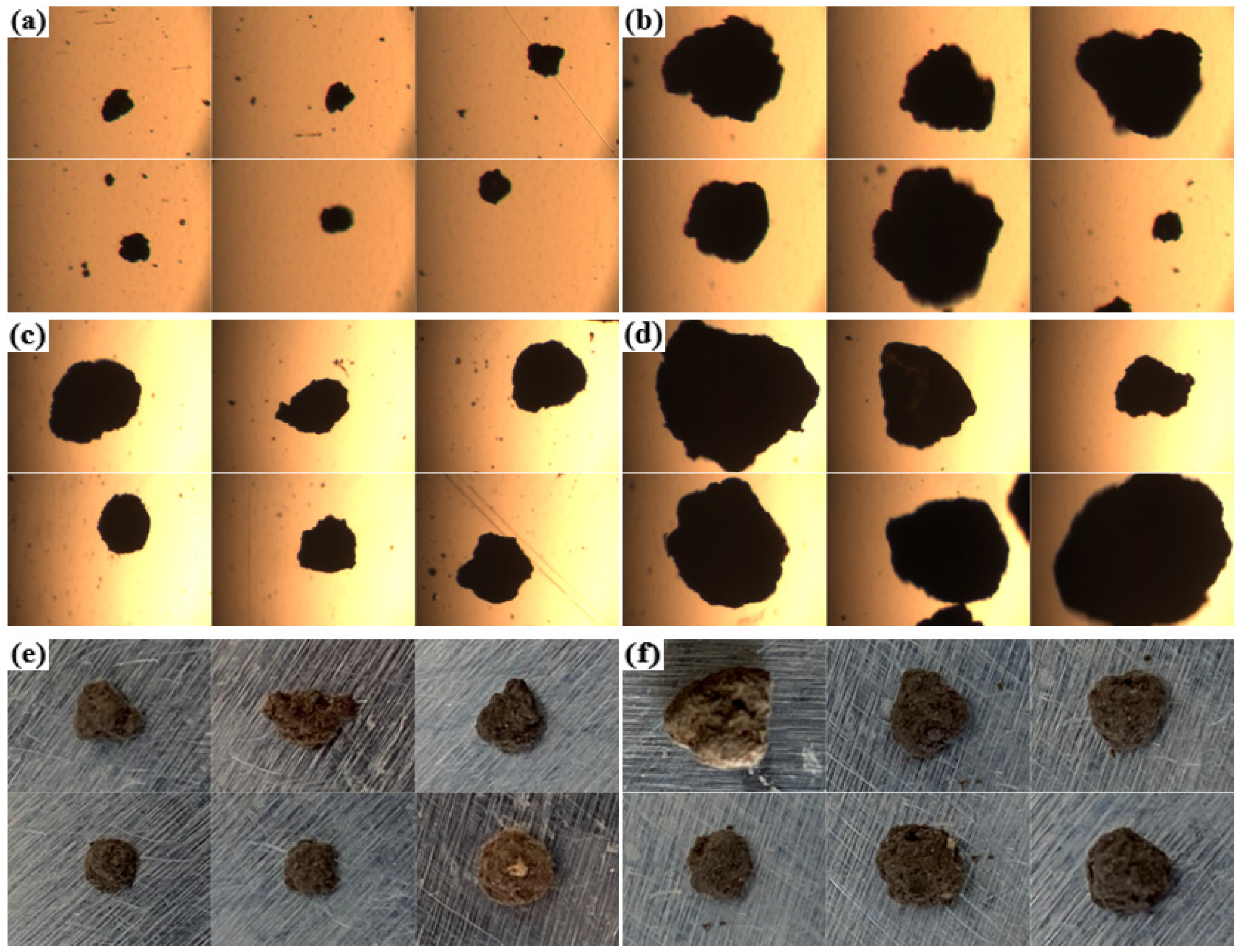Figure 3a–d show two-dimensional scanned images of representative soil particles of different particle size ranges selected for this paper. For soil particles in the particle size range of 1~2 mm and 2~3 mm, photographs were taken using a camera with 5× magnification, as shown in Figure 3e,f. The analysis in Figure 3 shows that the soil particles could be approximated as triangle-like and sphere-like in the different particle size ranges, and that both shapes accounted for the same proportion of the total mass.

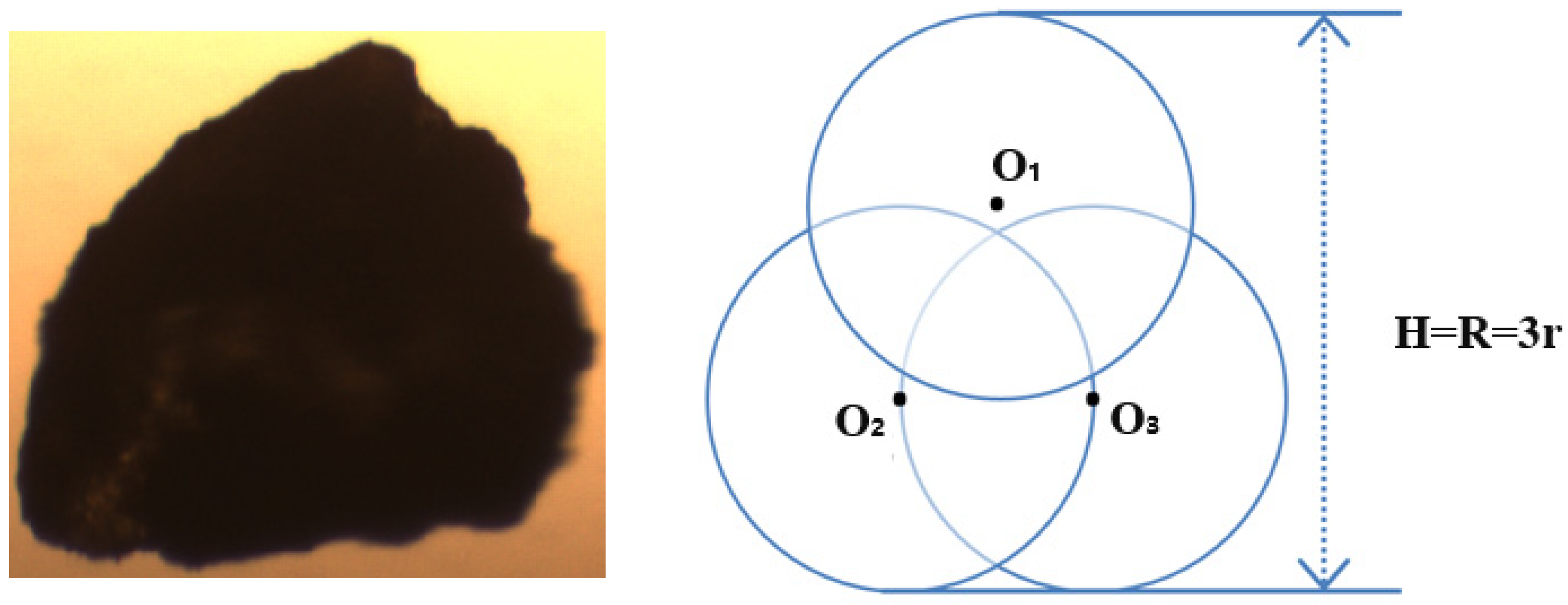
Geometric models of the two soil particle shapes described above were established. A large number of soil particles were required for simulation, so the number of constituent spheres in the particle model had to be reduced as much as possible.

For the triangle-like soil particles, three constituent spheres of the same radius (r) were used to model the geometry. The maximum distance H between the boundaries of the constituent spheres was defined as the current particle size R of the soil particles (H = R = 3r), as shown in Figure 4.

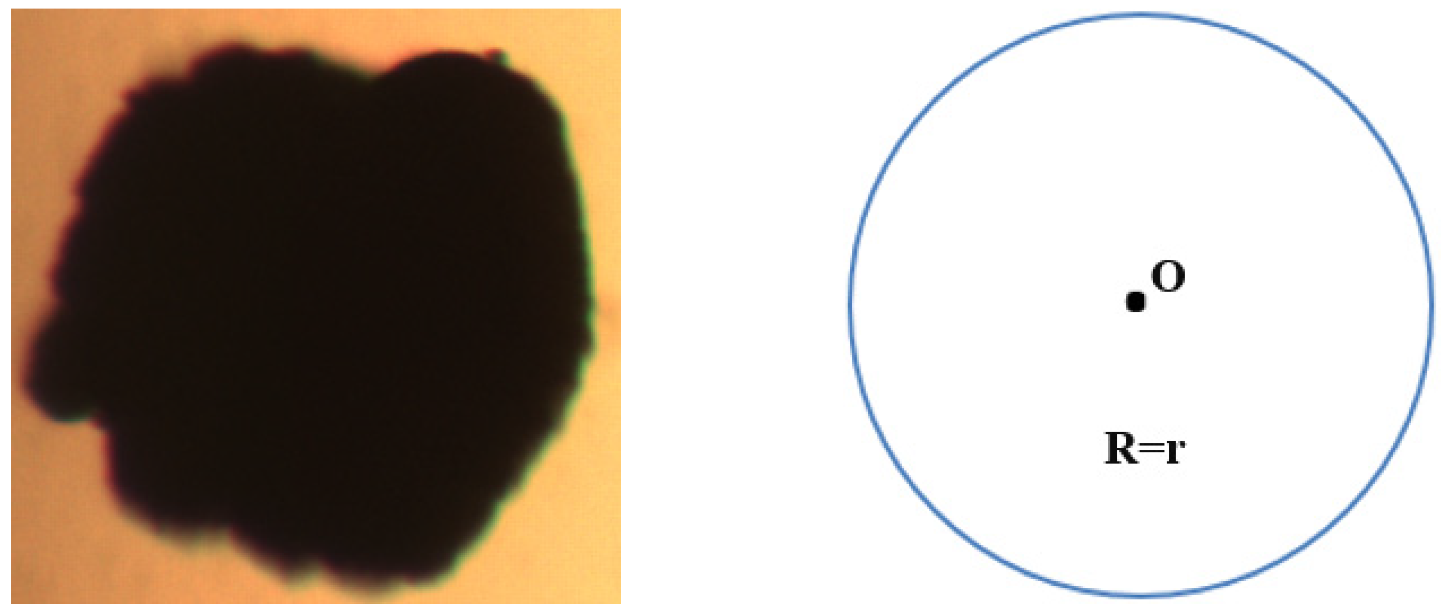
For the sphere-like soil particles, the geometric model was built directly using a single sphere with the same radius as the soil particles (R = r), as shown in Figure 5.

2.3. Particle Population Modeling

Following the particle size distribution of soil particles in the previous section, the mass ratio of soil particles with particle sizes ranging from 0 to 1 mm, 1 to 2 mm, and 2 to 3 mm could be approximated as 4:1:1. Therefore, when modeling the soil particle population, soil particles of different particle size ranges were generated in the proportions described above. A population of soil particles in the same particle size range was generated according to a uniform distribution using the middle size of each interval as the particle radius. In this way, the distribution of the modeled soil particle population was closer to that of the actual soil particle population.

The soil particles were small in size; however, the number of soil particles required for the simulation was relatively large. In order to make the soil particle model resemble actual soil more closely, and taking into account the duration and cost of the simulation, the particle diameter was chosen to be 1 mm, and a 1-sphere and 3-sphere model were generated in equal proportions so that the parameters of the simulation as well as the simulation results would be closer to the test values.

3. Measurement of Physical Parameters of Soil Particles

3.1. Measurement of Soil Moisture Content

The moisture content of the test soil was within 25% ± 1%, and, in accordance with the above test requirements, soil with a corresponding moisture content was configured in this study.

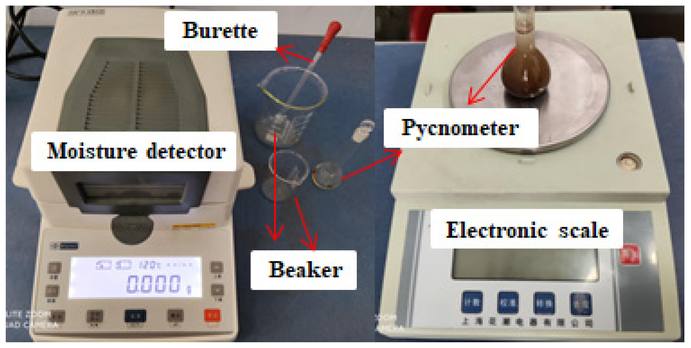
The moisture content measured by the XY-102MW halogen moisture analyzer is shown in Figure 6. The moisture content of the soil sample was measured by taking 3–5 g of the prepared soil and placing it on the tray of the moisture analyzer to be heated and dried. Three replicate tests were carried out, and the moisture content of the prepared soil was found to be 24.32%, which met the test requirements.

3.2. Measurement of Soil Particle Density

The type of density to be obtained for the EDEM simulation was the density of the soil particles, which was measured using the pycnometer method [12,13,14,15]. The test device is shown in Figure 6. The test was repeated three times to obtain a soil particle density of 1.841 g/cm³.

4. Direct Shear Test

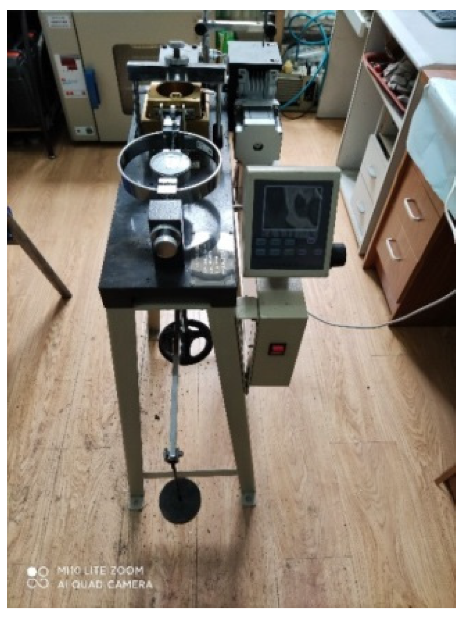
In this paper, the geometric model of soil particles was verified and the simulation parameters were calibrated by a direct shear test [16,17]. A ZJ-1B strain-controlled direct shear apparatus, as shown in Figure 7, which is an automatically controlled direct shear apparatus, was used to carry out the direct shear test of the soil.

The shear strength (τ) of the soil under different vertical loadings was measured by a direct shear test. The cohesion (c) and the internal friction angle (φ) were calculated as follows:

$$\tau =c+\sigma \tan \phi$$

(1)

The test procedure was as follows. We applied a vertical loading of 100 kPa and a shear speed of 2.4 mm/min and recorded the percent meter data every 30 s. When the percent meter was stable, we closed the forward button and recorded the data. The maximum shear strength (${\tau }_{\max }$) was calculated by the following formula:

$${\tau }_{\max }=C\ast R_f/\mathrm{A}$$

(2)

where C is the coefficient of the force ring, R_f is the reading of the percent meter when it is stable, and A is the cross-sectional area of the direct shear box.

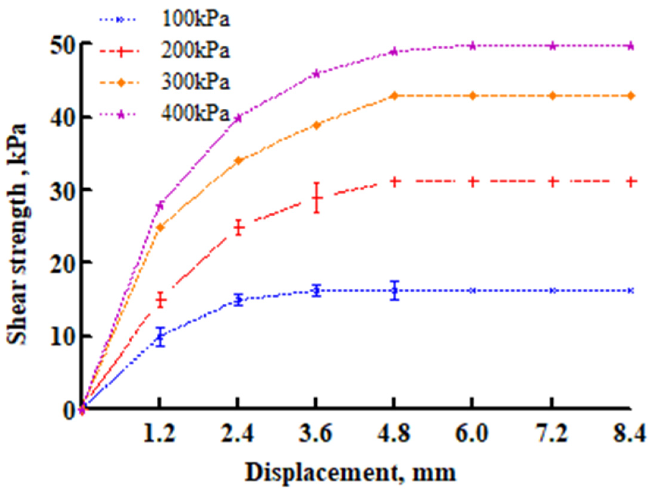
Three soil specimens were taken under vertical loadings of 100 kPa, 200 kPa, 300 kPa, and 400 kPa, and three tests were conducted for each. An image of the variation in shear strength with displacement for different vertical loading cases is shown in Figure 8.

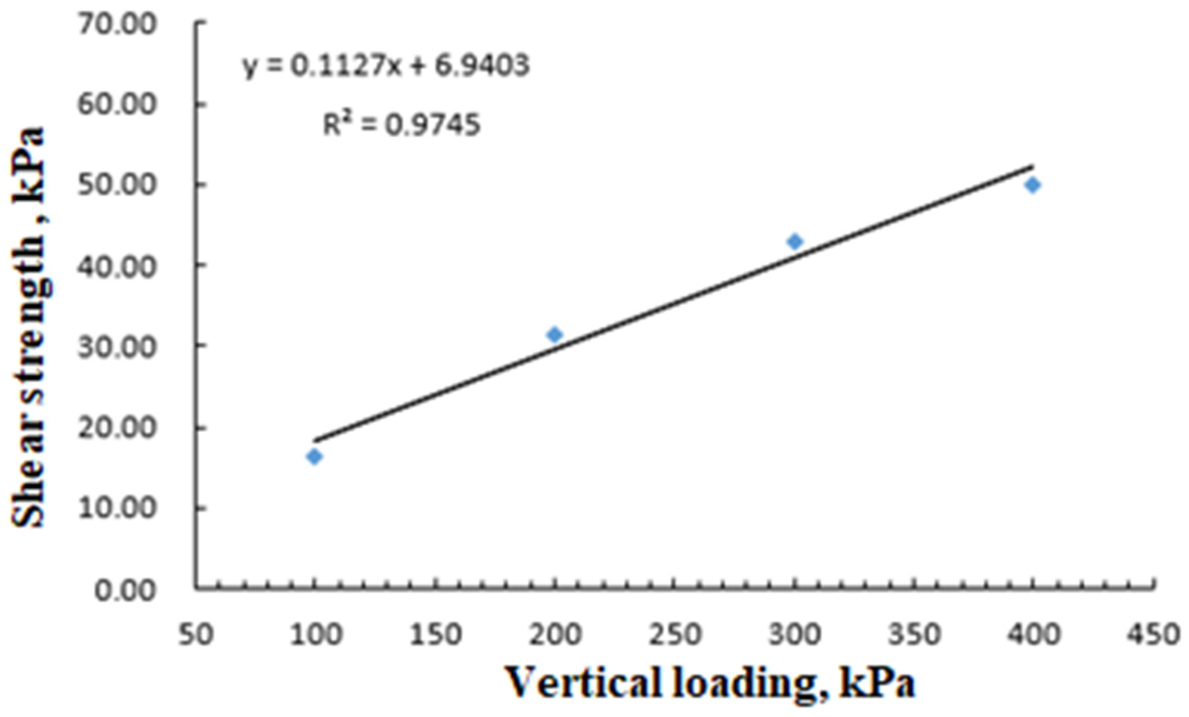
The relationship between the shear strength of the soil and the vertical loading is shown in Figure 9. The functional relationship can be expressed as:

y = 0.1127x + 5.9403 (R² = 0.9745)

(3)

The intersection of the straight line with the vertical coordinate represents the cohesive force (c) of the soil particles, the angle between the straight line and the horizontal coordinate is the angle (φ) of the internal friction of the soil, and the tangent of this angle is the slope of the corresponding straight line, as shown in Figure 9. Based on Equation (3), the cohesion and internal friction angle of the test soil were calculated to be 5.94 kPa and 5.43°, respectively.

5. The Simulation of Direct Shear Test

5.1. Simulation Analysis

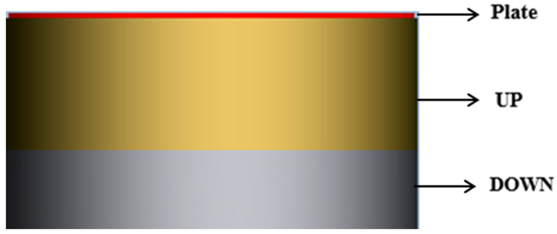
EDEM software was used to simulate the direct shear test. Figure 10 shows the geometric model of the DEM simulation. At the same time, the soil particles were modeled as a 1-sphere model and a 3-sphere model with a particle size of 1 mm. After generating soil particles in the straight shear box, simulation analysis was performed, and the steps are shown in detail below.

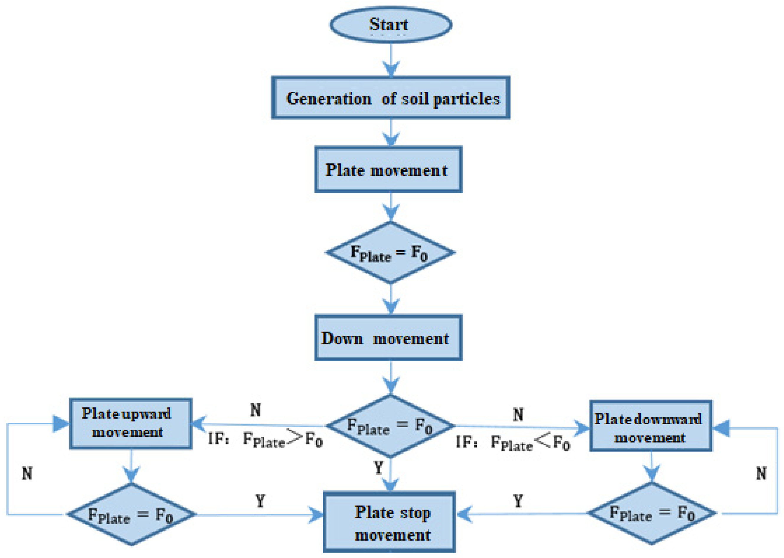
The loading in the vertical direction was constant during the test, and the requirement was achieved through the secondary development of the API. The program flow chart is shown in Figure 11. In the diagram, ${\mathrm{F}}_{\mathrm{Plate}}$ represents the force on the plate, and ${\mathrm{F}}_0$ represents the set value of the force applied to the plate.

5.2. Contact Model for Soil Particles

The four main contact models involved in soil particle simulation calculations are as follows. The Hertz–Mindlin model is suitable for non-compressible and non-sticky soil and materials such as dry gravel and sand. The Hertz–Mindlin with JKR model is suitable for non-compressible, sticky, or very sticky soil and materials such as wet gravel. The hysteretic spring model is suitable for compressible or very compressible dry soil and materials such as freshly ploughed soil. The EEPA model is suitable for compressible sticky or very sticky soil or soft, very sticky soil and materials such as clay and very wet sand [18,19,20,21,22].

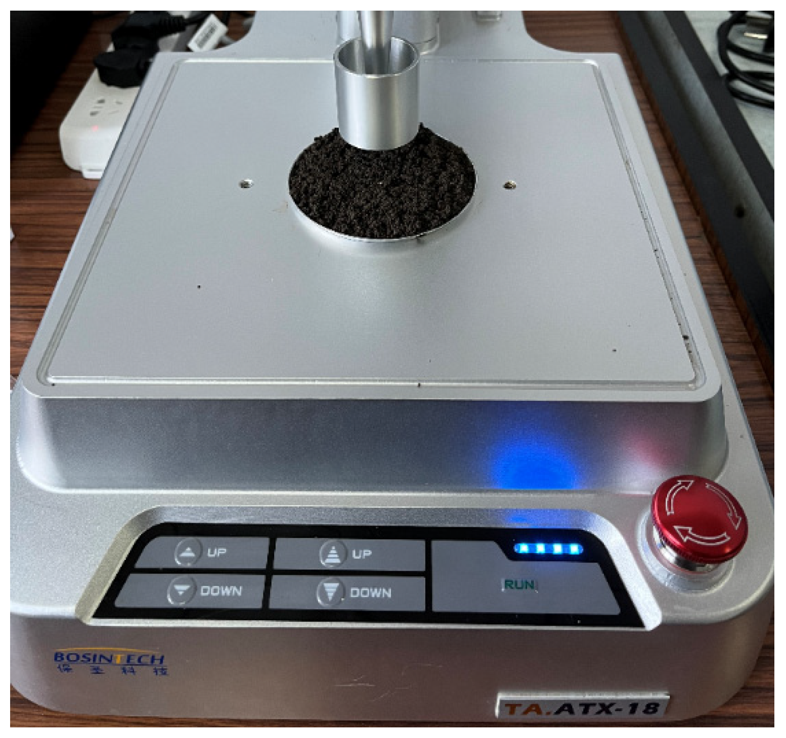
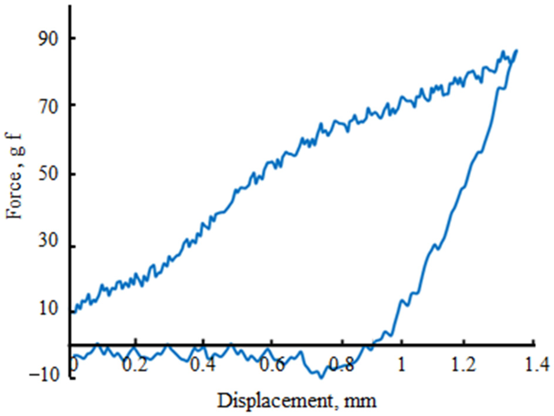
The test soil was a sandy loam with a moisture content of 25% ± 1%. The properties of the selected test soils were analyzed using a texture analyzer, as shown in Figure 12. The test procedure was as follows. The texture analyzer was calibrated, the test soil was placed in an aluminum foil soil tray, and the probe was moved downwards after starting the texture analyzer. After the probe had made contact with the soil, the force on the probe gradually increased. When the force reached its maximum, the moving probe started to travel in the opposite direction until it stopped.

The relationship between the force and the displacement of the probe is shown in Figure 13. Our analysis showed that when the displacement increased in the forward direction, the force gradually increased until it reached its maximum value. Conversely, when the displacement decreased, the force gradually decreased to zero, followed by the force increasing to its maximum and then gradually decreasing until it reached a relatively stable state. The above test analysis demonstrated that the test soil was a compressible and sticky material. The EEPA model was therefore used as the contact model for the test soil simulation in order to simulate the movement of the soil particles.

6. Calibration and Verification of Simulation Parameters

6.1. Introduction to the Simulation Parameters

The three categories of simulation parameters were as follows:

• The material parameters included the constituent spherical coordinates, density (ρ), shear modulus (G), and Poisson’s ratio (ν) of the soil particles and the density (ρ₀), shear modulus (G₀), and Poisson’s ratio (λ₀) of the boundary material.
• The parameters of interaction included the coefficient of static friction (μ₁), coefficient of rolling friction (μ₂), and coefficient of restitution (e) between soil particles, and the coefficient of static friction (μ₁₁), coefficient of rolling friction (μ₂₁), and coefficient of restitution (e₁) between soil particles and boundaries.
• The parameters of the EEPA model included the contact pull-off force (f₀), surface energy (γ), contact plastic ratio (λ), slope exp (n₀), tensile exp (n), and tangential stiff multiplier (k).

Some of the above parameters could be obtained directly by tests as well as by reference [16,17], as follows: ρ = 1843.9 kg/m³, G = 1 MPa, ν = 0.35, μ₁₁ = 0, μ₂₁ = 0, e₁ = 0.3, f₀ = 0, and n₀ = 1.5.

The rest of the parameters (μ_1, μ_2, e, γ, λ, n, and k) were calibrated by comparing the direct shear test with the simulation, and the response index was the shear strength.

6.2. Parameter Screening

The Plackett–Burman design (PBD) test was used to analyze the sensitivity of the parameters and to select the parameters that were sensitive to the response index. The PBD test is shown in

Table 2. Plackett–Burman design.

Standard Order	Run Order	Γ (J/m2)	λ	n	k	e	μ1	μ2
12	1	0.01	0.30	1	0.5	0.1	0.1	0.1
5	2	1.00	0.80	1	1.0	0.7	0.1	0.7
9	3	0.01	0.30	1	1.0	0.7	0.9	0.1
11	4	0.01	0.80	1	0.5	0.1	0.9	0.7
7	5	0.01	0.80	5	1.0	0.1	0.9	0.7
2	6	1.00	0.80	1	1.0	0.1	0.1	0.1
8	7	0.01	0.30	5	1.0	0.7	0.1	0.7
6	8	1.00	0.80	5	0.5	0.7	0.9	0.1
10	9	1.00	0.30	1	0.5	0.7	0.9	0.7
1	10	1.00	0.30	5	0.5	0.1	0.1	0.7
3	11	0.01	0.80	5	0.5	0.7	0.1	0.1
4	12	1.00	0.30	5	1.0	0.1	0.9	0.1

. The corresponding parameters were input into the EDEM software for simulation. Each set of parameters was simulated five times.

The factor analysis was carried out using the shear strength (τ) as the response index. Based on the analysis of variance of the PBD test, it could be seen that the p-value for the coefficient of static friction was 0.031, indicating that the coefficient of static friction was significant to the response index. The p-value for the surface energy was 0.184, and the p-value for the coefficient of rolling friction was 0.14, as shown in

Table 3. Analysis of variance of PBD test.

Source	Degree of Freedom	Adj SS	Adj MS	F-Value	p-Value
Model	7	945.56	135.081	2.69	0.178
Linear	7	945.56	135.081	2.69	0.178
γ (J/m2)	1	128.90	128.904	2.57	0.184
λ	1	50.47	50.471	1.01	0.373
n	1	60.17	60.166	1.20	0.335
k	1	2.99	2.990	0.06	0.819
e	1	0.29	0.291	0.01	0.943
μ1	1	533.47	533.467	10.64	0.031
μ2	1	169.28	169.275	3.37	0.140
Error	4	200.62	50.156
Total	11	1146.19

. These two parameters were approximately significant to the response index. The p-values for the other parameters were too large to have a significant effect on the response index.

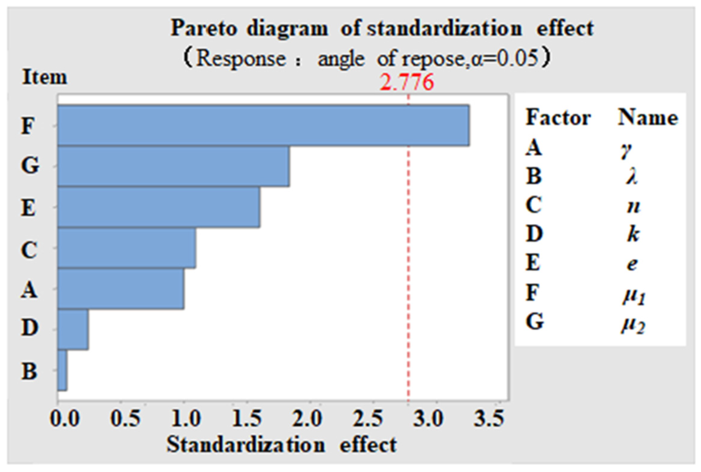
The Pareto diagram of the standardization effect of the PB test was analyzed, as shown in Figure 14. The histograms above the red dashed line indicate a significant effect on the response index. It is clear from the graph that the coefficient of static friction had a significant effect on the response index. The results for the coefficient of rolling friction and surface energy were closer to the red dashed line and had an approximately significant effect on the response index.

Based on the above analysis, the parameters to be calibrated in this paper were identified as the coefficient of static friction, the coefficient of rolling friction, and the surface energy.

6.3. Parameter Calibration

The response surface method was used to calibrate the above three parameters, and the other parameters were taken as follows: contact plastic ratio, λ = 0.35; coefficient of restitution, e = 0.5; tensile exp, n = 1; and tangential stiff multiplier, k = 1.

A three-factor Box–Behnken design (BBD) test was developed, as shown in

Table 4. Box–Behnken design.

Standard Order	Run Order	Vertex Type	District Group	μ1	μ2	γ
13	1	0	1	0.5	0.4	0.5
14	2	0	1	0.5	0.4	0.5
3	3	2	1	0.1	0.7	0.5
12	4	2	1	0.5	0.7	1.0
5	5	2	1	0.1	0.4	0.0
11	6	2	1	0.5	0.1	1.0
9	7	2	1	0.5	0.1	0.0
8	8	2	1	0.9	0.4	1.0
4	9	2	1	0.9	0.7	0.5
10	10	2	1	0.5	0.7	0.0
6	11	2	1	0.9	0.4	0.0
2	12	2	1	0.9	0.1	0.5
7	13	2	1	0.1	0.4	1.0
1	14	2	1	0.1	0.1	0.5
15	15	0	1	0.5	0.4	0.5

. The response index was the shear strength, with a simulated vertical loading of 100 kPa.

The corresponding parameters were entered into EDEM software for simulation. Each set of parameters was simulated five times, and the simulation results were analyzed. The analysis of variance for the BBD test showed that, for the model as a whole, with a p-value of 0.001, the predictive model of the test was extremely significant. For the linear analysis, the p-value of 0 for the coefficient of static friction had a significant effect on the response index. For the squared analysis, it could be seen that μ₁ × μ₁ had a p-value of 0.001, which had a significant effect on the response index. For the two-factor interaction analysis, it could be seen that μ₁ × μ₂ had a p-value of 0.031, which had a significant effect on the response index as shown in

Table 5. Analysis of variance for BBD test.

Source	Degree of Freedom	Adj SS	Adj MS	F-Value	p-Value
Model	9	1126.55	125.173	34.98	0.001
Linear	3	271.41	90.468	25.28	0.002
μ1	1	247.87	247.869	69.27	0.000
μ2	1	1.29	1.286	0.36	0.575
γ	1	0.08	0.079	0.02	0.887
Square	3	221.34	73.781	20.62	0.003
μ1 × μ1	1	215.97	215.965	60.36	0.001
μ2 × μ2	1	1.39	1.395	0.39	0.560
γ × γ	1	0.81	0.808	0.23	0.655
Two-factor interaction	3	43.38	14.460	4.04	0.083
μ1 × μ2	1	31.92	31.922	8.92	0.031
μ1 × γ	1	11.46	11.458	3.20	0.134
μ2 × γ	1	0.00	0.000	0.00	0.992
Error	5	17.89	3.578
Lack of fit	3	9.31	3.103	0.72	0.625
Pure error	2	8.58	4.291
Total	14	1144.45

.

The analysis of the model for the BBD test showed that the R-sq value reached 98.44%, indicating a very good fit, as shown in

Table 6. Analysis of model for BBD test.

S	R-sq	R-sq (Adjustment)	R-sq (Predictions)
1.89161	98.44%	95.62%	85.30%

.

The corresponding regression equation was further obtained, and the formula was as follows:

τ = 11.61 + 86.7 μ₁ − 6.2 μ₂ + 0.75 γ − 127.4 μ₁ × μ₁ + 10.2 μ₂ × μ₂ − 1.87 γ × γ + 47.1 μ₁ × μ₂ + 13.82 μ₁ × γ + 0.08 μ₂ × γ

(4)

In the direct shear test, when the vertical loading was 100 kPa, the corresponding shear strength was 16.25 kPa. Firstly, the range of parameters was determined, wherein the coefficient of static friction was 0.1~0.9, the coefficient of rolling friction was 0.1~0.7, and the surface energy was 0~1 J/m². Next, the parameters were optimized for the constrained range, and the final values of 0.9, 0.7, and 1 J/m² were calibrated for the coefficient of static friction, the coefficient of rolling friction, and the surface energy, respectively.

6.4. Validation of Calibration Parameters

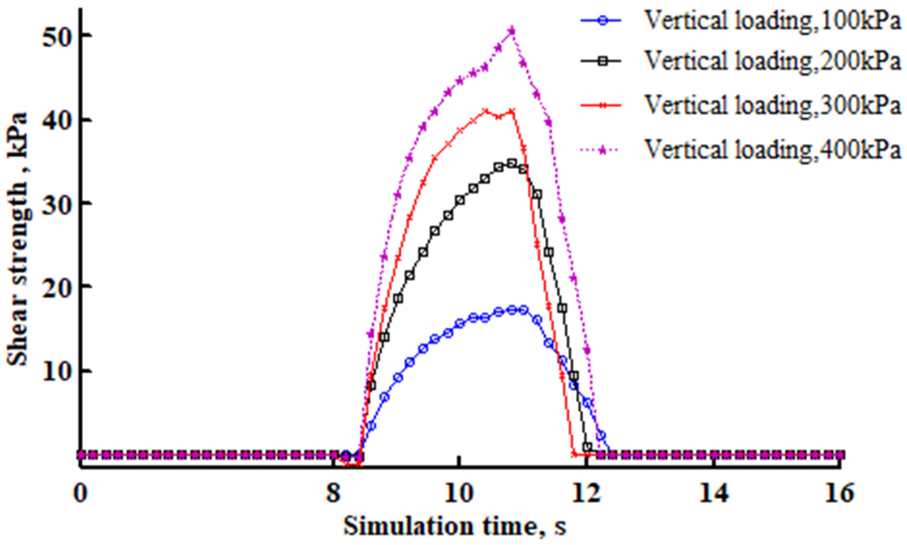
To verify the accuracy of the calibration parameters, the shear strength of the soil was simulated and calculated for vertical loadings of 100 kPa, 200 kPa, 300 kPa, and 400 kPa. The relationship between the shear strength and the simulation time of the soil particles for the direct shear simulation is shown in Figure 15. When the shear box started to move, shear strength was generated, which gradually increased and started to decrease after reaching a maximum value, and the simulation recorded the shear strength under different loadings.

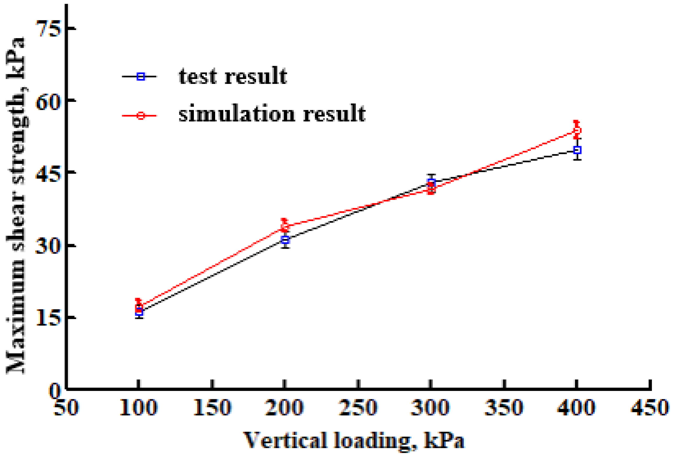
Figure 16 shows a comparison of the simulation and test results for the maximum shear strength under different vertical loadings. As the vertical loading increased, the maximum shear strength of the soil particles gradually increased, and the simulation and test results showed the same trend. When the vertical loading was 100 kPa, the average value of the simulation result was slightly higher than the test result, with a difference of 1.22 kPa. When the vertical loading was 200 kPa, the average value of the simulation result was also slightly higher than the test result, with a difference of 2.77 kPa. When the vertical loading was 300 kPa, the average value of the simulation result was slightly lower than the test result, with a difference of 1.26 kPa. When the vertical loading was 400 kPa, the average value of the simulation result was slightly higher than the test result, with a difference of 4 kPa. The analysis showed that the simulation and test values of the maximum shear strength of the soil particles were very close to each other for the same loading. The percentage difference between the simulation and the test results was greatest when the vertical loading was 200 kPa. The value was 8.8% < 10%, which is within the acceptable deviation range.

The results of the direct shear test were compared with the relevant reference [23,24]. It could be seen that the maximum shear strength was different under different vertical loadings due to the different soil materials tested. However, the trends of the test results in this paper and the corresponding reference results were the same.

The above analysis showed that the results of the calibration parameters for the soil particles in this paper were correct. The parameters were taken as e = 0.3, λ = 0.35, n = 1, k = 0.67, μ₁ = 0.9, μ₂ = 0.7, and γ = 1 J/m².

7. Conclusions

In this paper, a systematic analysis of the test soil was carried out, and a geometric model of the soil was established. The EEPA model was identified as the contact model, and the parameters were calibrated. The accuracy of the calibrated parameters and the geometric model of the soil particles was verified. The main conclusions are presented below:

(1) The geometry of the test soil was analyzed using an image particle analyzer, which approximated the soil particles as sphere-like and triangle-like and established a geometric model of the soil particles.

(2) Soil with a moisture content of 25% ± 1% was configured according to the test requirements; the density of soil particles was measured using the pycnometer method to be 1.844 g/cm³.

(3) The physical properties—compressibility and stickiness—of the soil used for the test were demonstrated by texture tests, and the EEPA model was chosen as the contact model for the soil particle simulation.

(4) A direct shear test was used to calibrate the corresponding parameters using shear strength as the response index. Firstly, the sensitivity of the parameters was analyzed through PB tests, and it was determined that the coefficient of static friction had a significant effect on the response index and that the surface energy and the coefficient of rolling friction had an approximately significant effect on the response index. Next, the BBD test was developed to calibrate the three parameters mentioned above by the response surface method, and the optimized parameter values were obtained. The applicability and accuracy of the parameters were further determined by comparing the simulation and test results of the direct shear test under different loadings, and the applicability of the soil particle model was also verified.

References

- Cundall, P.A.; Burman, B.C.; Strack, O.D.L. A discrete numerical model for granular assemblies. Géotechnique 1980, 30, 331–336. [Google Scholar] [CrossRef]
- Yan, D.; Yu, J.; Wang, Y.; Zhou, L.; Sun, K.; Tian, Y. A Review of the Application of Discrete Element Method in Agricultural Engineering: A Case Study of Soybean. Processes 2022, 10, 1305. [Google Scholar] [CrossRef]
- Zeng, Z.W.; Ma, X.; Cao, X.L.; LI, Z.H.; Wang, X.C. Critical Review of Applications of Discrete Element Method in Agricultural Engineering. Trans. Chin. Soc. Agric. Mach. 2021, 52, 1–18. [Google Scholar]
- Yu, Y.J.; Fu, H.; Yu, J.Q. DEM-based simulation of the corn threshing process. Adv. Powder Technol. 2015, 26, 1400–1409. [Google Scholar] [CrossRef]
- Xu, T.Y.; Yu, J.Q.; Yu, Y.J.; Wang, Y. A modelling and verification approach for soybean seed particles using the discrete element method. Adv. Powder Technol. 2018, 29, 3274–3290. [Google Scholar] [CrossRef]
- Yan, D.; Yu, J.; Zhang, N.; Tian, Y.; Wang, L. Test and Simulation Analysis of Soybean Seed Throwing Process. Processes 2022, 10, 1731. [Google Scholar] [CrossRef]
- Ucgul, M.; Fielke, J.M.; Saunders, C. Three-dimensional discrete element modelling of tillage: Determination of a suitable contact model and parameters for a cohesionless soil. Biosyst. Eng. 2014, 121, 105–117. [Google Scholar] [CrossRef]
- Bravo, E.L.; Tijskens, E.; Suárez, M.H.; Cueto, O.G.; Ramon, H. Prediction model for non-inversion soil tillage implemented on discrete element method. Comput. Electron. Agric. 2014, 106, 120–127. [Google Scholar] [CrossRef]
- Chen, Y.; Munkholm, L.J.; Nyord, T. A discrete element model for soil–sweep interaction in three different soils. Soil Tillage Res. 2013, 126, 34–41. [Google Scholar] [CrossRef]
- Xiang, W.; Wu, M.L.; Lü, J.N.; Quan, W.; Ma, L.; Liu, J.J. Calibration of simulation physical parameters of clay loam based on soil accumulation test. Trans. Chin. Soc. Agric. Eng. 2019, 35, 116–123. [Google Scholar]
- Lu, R.K. Methods of Agricultural Chemical Analysis of Soils; China Agricultural Science and Technology Press: Beijing, China, 2000. [Google Scholar]
- Ogunjimi, L.A.; Aviara, N.A.; Aregbesola, O.A. Some engineering properties of locust bean seed. J. Food Eng. 2002, 55, 95–99. [Google Scholar] [CrossRef]
- Aviara, N.A.; Gwandzang, M.I.; Haque, M.A. Physical Properties of Guna Seeds. J. Agric. Eng. Res. 1999, 73, 105–111. [Google Scholar] [CrossRef]
- Omobuwajo, T.O.; Akande, E.A.; Sanni, L.A. Selected physical, mechanical and aerodynamic properties of African breadfruit (Treculia africana) seeds. J. Food Eng. 1999, 10, 241–244. [Google Scholar] [CrossRef]
- Al-Mahasneh, M.A.; Rababah, T.M. Effect of moisture content on some physical properties of green wheat. J. Food Eng. 2007, 79, 1467–1473. [Google Scholar] [CrossRef]
- Mousaviraad, M.; Tekeste, M.Z.; Rosentrater, K.A. Calibration and Validation of a Discrete Element Model of Corn Using Grain Flow Simulation in a Commercial Screw Grain Auger. Trans. ASABE 2017, 60, 1403–1415. [Google Scholar] [CrossRef]
- Wang, X.L.; Hu, H.; Wang, Q.G.; Li, H.W.; He, J.; Chen, W.Z. Calibration Method of Soil Contact Characteristic Parameters Based on DEM Theory. Trans. Chin. Soc. Agric. Mach. 2017, 48, 78–85. [Google Scholar]
- Boac, J.M.; Ambrose, R.P.K.; Casada, M.E.; Maghirang, R.G.; Maier, D.E. Applications of Discrete Element Method in Modeling of Grain Postharvest Operations. Food Eng. Rev. 2014, 6, 128–149. [Google Scholar] [CrossRef]
- Shi, L.R.; Zhao, W.Y.; Sun, W. Parameter calibration of soil particles contact model of farmland soil in northwest arid region based on discrete element method. Trans. Chin. Soc. Agric. Eng. 2017, 33, 181–187. [Google Scholar]
- Ma, Y.J.; Wang, A.; Zhao, J.G.; Hao, J.J.; Li, J.C.; Ma, L.P.; Zhao, W.B.; Wu, Y. Simulation analysis and experiment of drag reduction effect of convex blade subsoiler based on discrete element method. Trans. Chin. Soc. Agric. Eng. 2019, 35, 16–23. [Google Scholar]
- Landry, H.; Laguë, C.; Roberge, M. Discrete element representation of manure products. Comput. Electron. Agric. 2006, 51, 17–34. [Google Scholar] [CrossRef]
- Ai, J.; Chen, J.F.; Rotter, J.M.; Ooi, J.Y. Assessment of Rolling Resistance Models in Discrete Element Simulations. Powder Technol. 2011, 206, 269–282. [Google Scholar] [CrossRef]
- Pascale, C. Rouse. Relation between the critical state friction angle of sands and low vertical stresses in the direct shear test. Soils Found. 2018, 10, 1282–1287. [Google Scholar]
- Jiang, Y.; Li, Y.J.; Xu, Y. Discrete Element Simulation of Direct Shear Test of Sandy Silt Soils. Soil Eng. Found. 2017, 31, 4. [Google Scholar]
Figure 1.
Standard soil sieve.
Figure 2.
XS-2100 image particle analyzer.
Figure 3.
Enlarged view of soil particles in different size ranges: (a) 0~0.075 mm, (b) 0.075~0.25 mm, (c) 0.2~0.5 mm, (d) 0.5~1 mm, (e) 1~2 mm, and (f) 2~3 mm.
Figure 4.
Modeling of triangle-like soil particle.
Figure 5.
Modeling of sphere-like soil particle.
Figure 6.
Soil moisture content and particle density test device.
Figure 7.
ZJ-1B direct shear apparatus.
Figure 8.
The relationship between shear strength and displacement under different vertical loadings.