HBRNet: Boundary Enhancement Segmentation Network for Cropland Extraction in High-Resolution Remote Sensing Images

Abstract

Cropland extraction has great significance in crop area statistics, intelligent farm machinery operations, agricultural yield estimates, and so on. Semantic segmentation is widely applied to remote sensing image cropland extraction. Traditional semantic segmentation methods using convolutional networks result in a lack of contextual and boundary information when extracting large areas of cropland. In this paper, we propose a boundary enhancement segmentation network for cropland extraction in high-resolution remote sensing images (HBRNet). HBRNet uses Swin Transformer with the pyramidal hierarchy as the backbone to enhance the boundary details while obtaining context. We separate the boundary features and body features from the low-level features, and then perform a boundary detail enhancement module (BDE) on the high-level features. Endeavoring to fuse the boundary features and body features, the module for interaction between boundary information and body information (IBBM) is proposed. We select remote sensing images containing large-scale cropland in Yizheng City, Jiangsu Province as the Agricultural dataset for cropland extraction. Our algorithm is applied to the Agriculture dataset to extract cropland with mIoU of 79.61%, OA of 89.4%, and IoU of 84.59% for cropland. In addition, we conduct experiments on the DeepGlobe, which focuses on the rural areas and has a diversity of cropland cover types. The experimental results indicate that HBRNet improves the segmentation performance of the cropland.

1. Introduction

Appropriate planning area and geographical location of cropland is the potential for increasing agricultural production and efficiency, as well as a fundamental initiative to ensure national grain security [1,2]. Many important agricultural applications, such as crop yield prediction, unmanned farm construction, and farm equipment path planning, require the area and distribution of cropland.

The traditional way of manually measuring cropland is labor-intensive and time-consuming [3,4,5]. Therefore, an intelligent way of cropland extraction is urgently demanded. By extracting cropland from high-resolution remote sensing images, we can rapidly, distinctly, and intuitively capture the area of cropland and its distribution [6,7]. The classical image segmentation method to extract cropland requires manual design of features, which is difficult and not universally applicable due to the feature diversity of high- resolution remotely sensed images. The deployment of deep learning algorithms for cropland extraction has witnessed some remarkable progress.

Semantic segmentation algorithm is an essential technique to extract cropland from remotely sensed images [8], primarily by classifying the pixels of images to predict the distribution of cropland. In the procedure of extracting cropland, the boundary information of cropland takes an active role. High-resolution images provide abundant image details, which facilitates the acquisition of boundary information of cropland [9,10,11]. However, the shape of cropland observed on remote sensing images is similar to that of artificial lakes and small forests, and the local pixel information is similar to that of wasteland. In case the cropland is present in areas with complex terrain such as hills, woodlands, and lakes, it would be more challenging to extract. Hence, contextual information and boundary information have a positive contribution to improve the accuracy of cropland extraction.

Semantic segmentation usually requires cropping and downsampling operations during the training process of convolutional neural networks (CNNs). These operations will result in the loss of context and details of the image. Limited by the receptive field size of the convolutional kernel, CNNs only model local information of the image (e.g., local color, texture) [12,13], while ignoring the global contextual information of the image [14,15]. Moreover, the multiple scales of objects can lead to a lack of context [16]. Hierarchical pyramidal structure networks and attention mechanisms are commonly used to solve feature aggregation [17,18,19,20]. Zheng et al. [13] applied Transformer to the semantic segmentation algorithm. The local attention mechanism significantly improves computational efficiency and achieves significant improvements semantic segmentation tasks [21,22]. Liu et al. [23] proposed a hierarchical vision transformer with shifted windows, which can effectively achieve the aggregation of context features. Swin transformer is a deep learning method that differs from CNNs, in that it is based on a self-attention mechanism. Swin transformer is quite a new approach, but it has been widely used in real-life applications due to its ability to achieve promising results in semantic segmentation. The ability of the Swin transformer to effectively tackle the challenge of extracting contextual information in semantic segmentation tasks information, which motivates us to want to use it as a backbone for extracting cropland. However, there is a drawback in the refinement of image boundary details when applying Swin Transformer to cropland extraction.

The performance of high-resolution remotely sensed images semantic segmentation is limited by spatial resolution and fuzzy boundary information [24,25,26]. Therefore, it is extremely important to extract and refine boundary features in an accurate way [27]. There are three main approaches for boundary refinement. First, a backbone network is proposed for local detail refinement, which can reduce boundary artifacts and refine the mask profile during the final high-resolution mask generation [28]. Second, the boundary refinement for the generated prediction maps is performed to obtain clearer information about the boundary features [29]. Third, it is designed as a discrete refinement module to improve boundary accuracy [18]. The refinement module is usually a boundary refinement for high-level features, as shown in Figure 1a, or a boundary refinement for low-level features, as shown in Figure 1b. These methods of boundary enhancement based on single-level features ignores the complementarity of effective features between different level features. Optionally fusing different level features can help to obtain more boundary information. Although the low-level features contain more boundaries due to their higher resolution, there are cases where the boundaries are blurred and difficult to extract accurately. Therefore, we propose a refinement module to refine the boundary of different level features. As shown in Figure 1c, the boundary refinement module is first applied to the two level features, and then the boundary-enhanced features are fused to obtain the prediction maps. After completing the hierarchical boundary refinement, we combine two level features to obtain clearer boundaries.

In this paper, we use Swin Transformer with hierarchical structure as the backbone to perform hierarchical boundary refinement for two level features. This hierarchical enhancement improves the extraction of farmland boundaries and makes it easier to distinguish between farmland and background. We designed a cross-detail module to realize the interaction between local information and global information when recovering resolution information. The interaction of global and local information is intended to better highlight the distinguishing features between farmland information and background information. In hierarchical network, low-level features tend to contain higher resolution, but extracted context is missing, resulting in low-level features negatively affecting the overall prediction results [9,30]. In contrast, high-level features undergo multi-scale transformations to obtain richer context information [31,32]. The differences in resolution and processing modules result in different information being obtained for the features in different layers. The accuracy of segmentation can be effectively improved by applying a unique feature enhancement module to each layer of features separately and then performing feature fusion.

In order to maintain as many details as possible in the high-resolution features, the boundary body separation module is used to extract the rich details from the low-level features. We propose a boundary detail enhancement module (BDE) for enhancing the boundary information of high-level features, which uses cross-convolution to obtain more boundary information from both horizontal and vertical directions in parallel. Compared with the traditional convolution network, cross convolution can obtain more detailed information. After the boundary refinement is achieved in the high-level features, the boundaries are combined with those in the low-level features to generate feature maps with more details. In addition, the efficient way to combine the extracted boundary features with the body features is also a crucial part. In order to share and complement the information between the two features, we propose the module for interaction between boundary information and body information (IBBM) to combine boundary information and body features. IBBM is performed between the high-level feature map after boundary enhancement and the body features extracted from the low-level feature map, and feature fusion is realized through the IBBM. This interaction method mainly focuses on the interaction of local information, which can effectively realize the effective combination of boundary information and body features. Inspired by Walid et al. [33], we propose a cross-detail module with cross-attention. Local features and global features have different definitions, and basic concatenation would not interact between features [34]. To enhance the interactivity and degree of association between global and local features, we embed the cross-attention mechanism to refine the multi-layer perceptron (MLP). Contrary to unidirectional context acquisition, cross-attention achieves interaction between contextual and global information, which leads to better recovery of high-resolution feature maps.

We conduct cropland extraction experiments on two datasets (Agriculture and DeepGlobe [35]). Our method, the boundary enhancement segmentation network for cropland extraction in high-resolution remote sensing images (HBRNet), achieves state-of-the-art performances on two datasets (Agriculture and DeepGlobe). The main contributions of this paper are as follows:

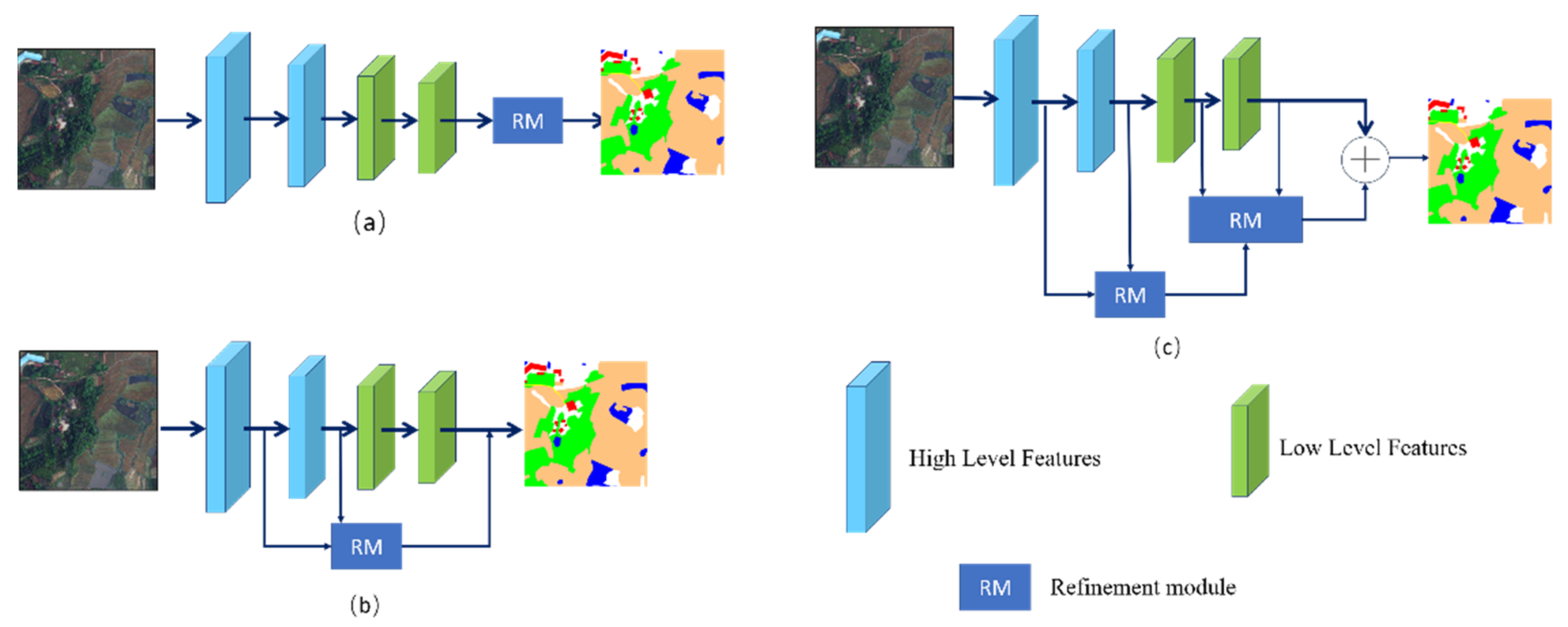
• In order to better distinguish between cropland features non-cropland features, we hierarchically refined the boundary information for multi-level network structures. For high-level features, we implemented the enhancement of boundary features while obtaining contextual information as much as possible. For low-level features with higher resolution, we used boundary-body separation module to extract boundary information and body information.
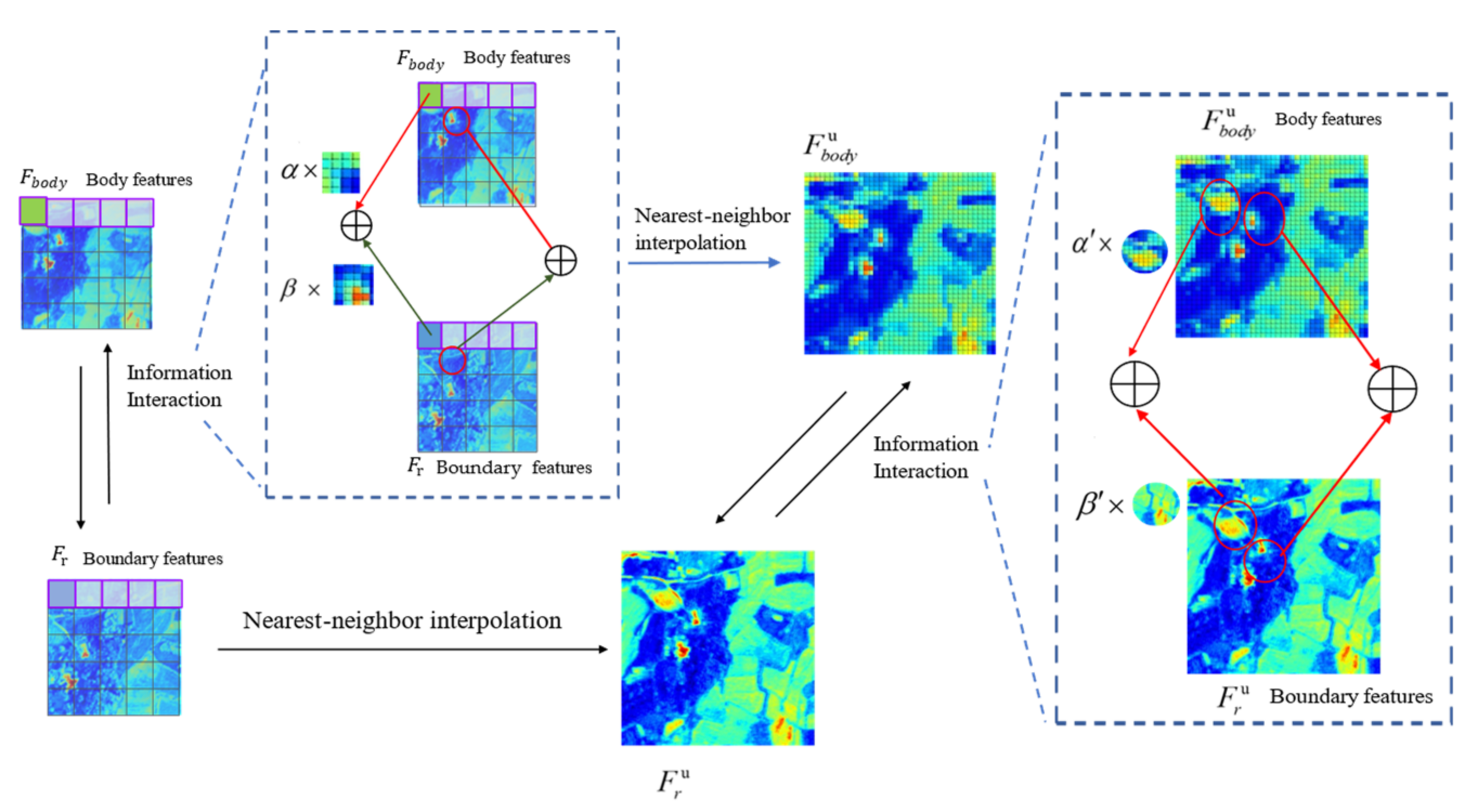
• We designed a boundary detail enhancement module (BDE), which is applied to high-level features that obtain more global information. This enhancement highlights the information on the boundaries of the cropland more conducive to cropland extraction. After completing the boundary feature enhancement, we proposed an information interaction module (IBBM) for feature interaction between boundary features and body features to obtain a more precise feature map.
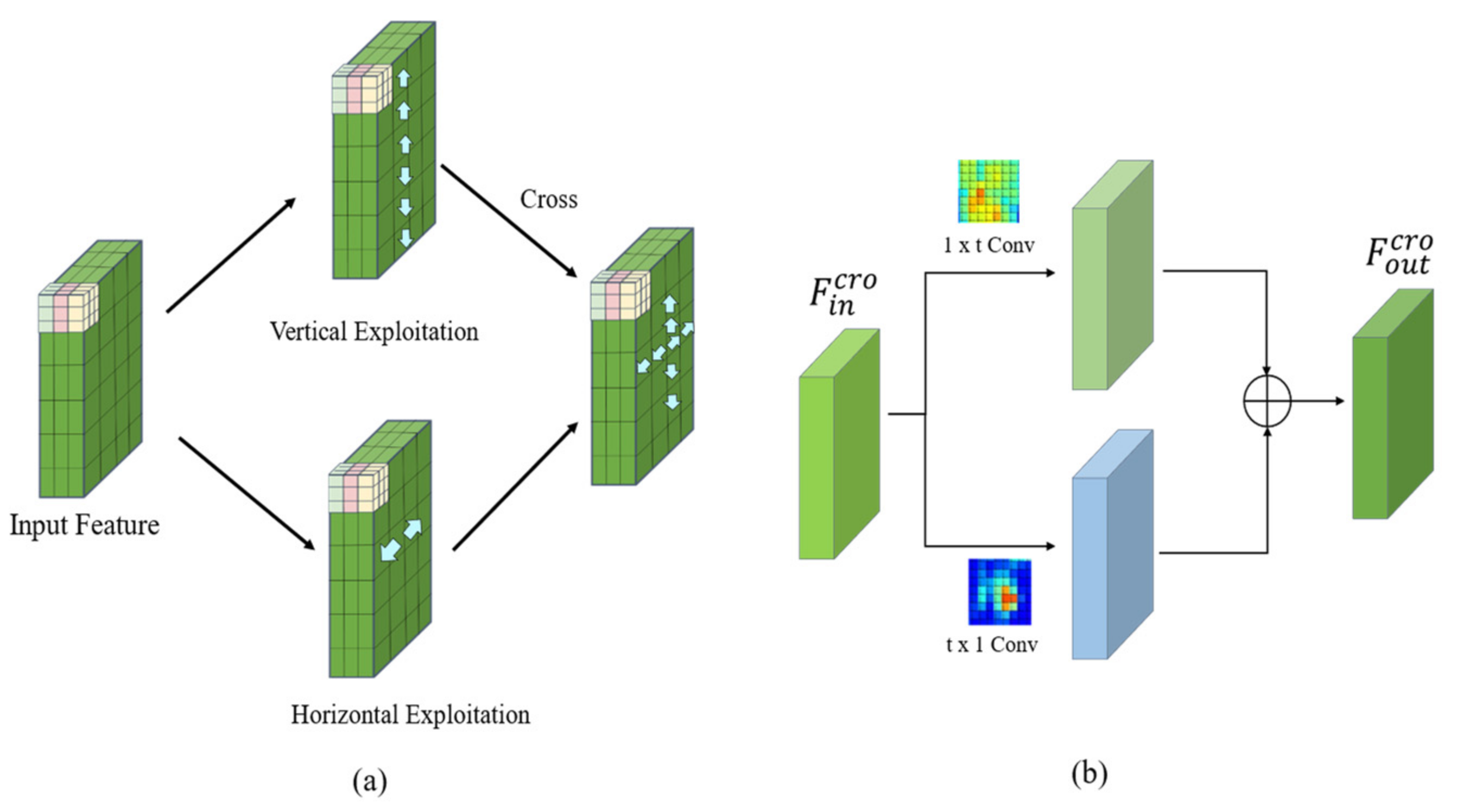
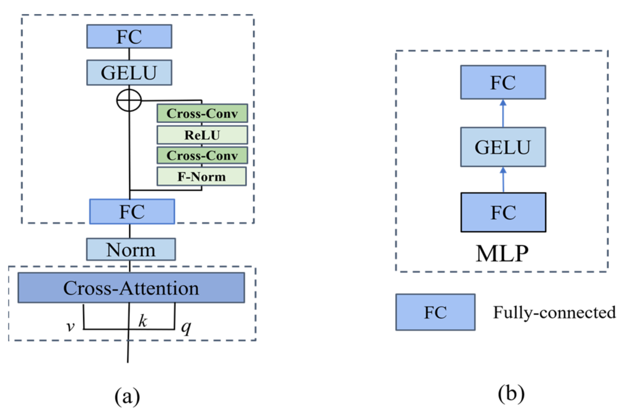
• We propose a cross-detail module by combining the cross-attention mechanism with an improved multi-layer perceptron (MLP). We set up the detail branch to the MLP layer, which makes it possible to enhance the detail information of the extracted features.

2. Materials and Methods

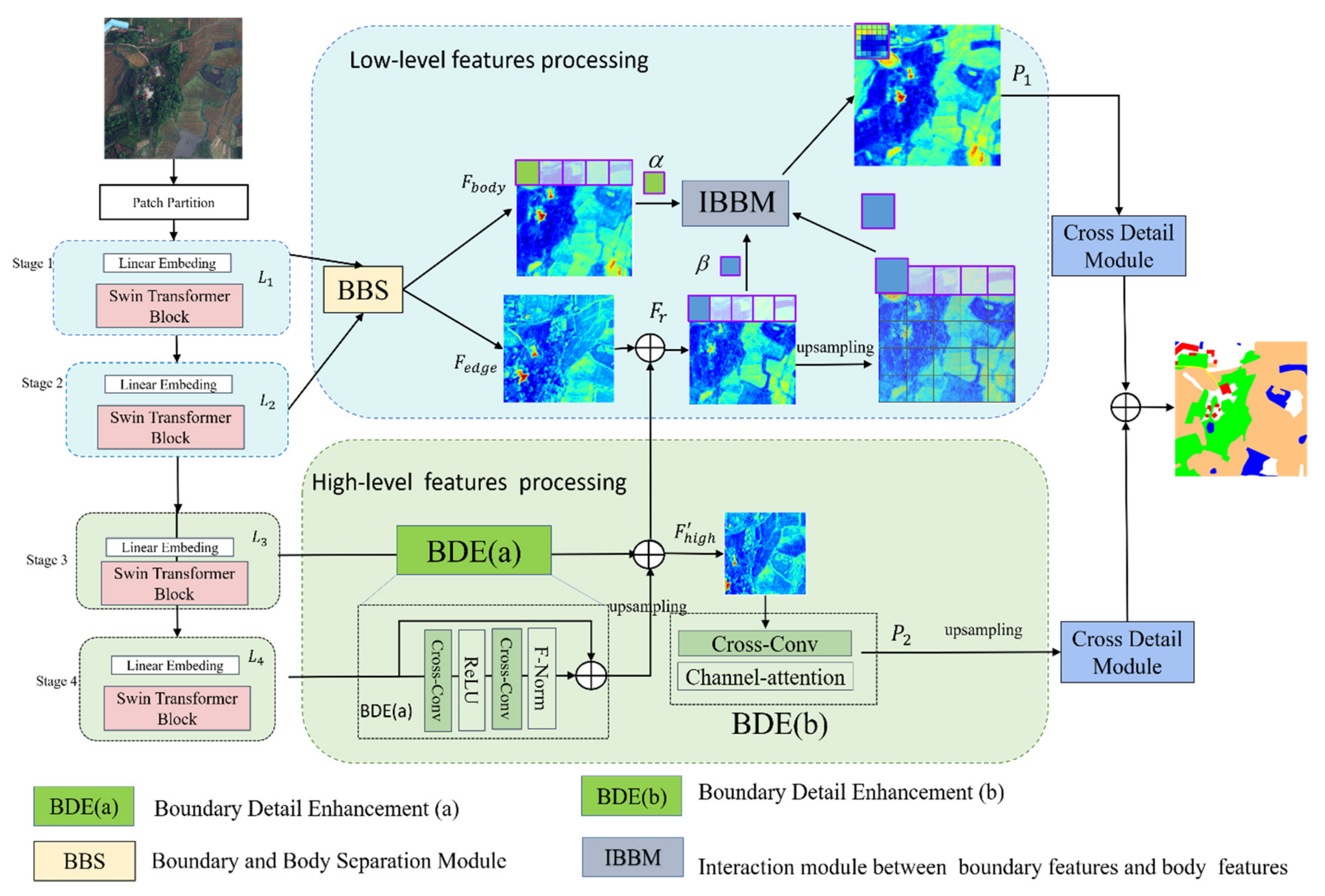
2.1. Network Architecture

HBRNet mainly focuses on boundary refinement in different ways for each layer of the output feature map in the backbone network. The backbone of the network is Swin Transformer, and the two successive Swin Transformer blocks are shown in Figure 2.

Swin Transformer segments the input image into non-overlapping patches and consider each patch as a “token”. We employed a patch size of 4 × 4 as described in [23], thus calculating a feature dimension of 48 for each patch. Apply a linear embedding layer to the raw-valued features, projecting it to an arbitrary dimension (denoted as C). The Swin Transformer contains 4 main levels, each level with a different number of transformer blocks. The patch merging merges tokens to generate different numbers of tokens and thus combines them into different resolution features. Several modified transformer blocks are applied to these patch markers and their self-attention computations are performed. Each group concatenates features from 2 × 2 of the neighboring patches to produce a 4C-dimensional feature series. The 4C-dimensional tandem features are passed through a linear layer to generate the first patch merge layer. After that, the token is reduced by a factor of 4 according to the downsampling rate of the resolution, then the output dimension can be set to $2C$. The resolutions of the feature map output from Stage 2, 3, and 4 after feature transformation blocks are $\mathrm{H}/8 \times \mathrm{W}/8$, $\mathrm{H}/16 \times \mathrm{W}/16$, and $\mathrm{H}/32 \times \mathrm{W}/32$. In this paper, we denote the output features of Swin Transformer from the first stage to the fourth stage as $\left\{L_1,L_2,L_3,L_4\right\}$. In this paper, the Swin-Tiny variation network (Swin-T) is used as the backbone, where the dimension C is 96, the numbers of Swin Transformer blocks in each stage are $\left\{2,2,6,2\right\}$. As shown in Figure 2, the two consecutive Swin Transformer blocks are mainly composed of window-based multi-head self-attention and shifted window-based multi-head self-attention. It is obvious from the figure that a multi-head self-attention module is included between every two Layer Norm layers.

We utilized the agricultural cropland image as our image input. Firstly, we generated the feature maps for the different layers according to the four stages in the backbone, i.e., Figure 3. Secondly, we applied different processing methods to the different layers of features. Thirdly, by combining the features of each layer, we obtained an extracted image of the cropland with more boundary detail. It is worth mentioning that the processing we specify for the different layers of features is customized, taking into account the unique characteristic of each layer of in the module. Therefore, the fusion of the final features allows the results of each layer to complement each other and thus retain more detailed information when extracting the cropland.

As shown in Figure 3, we upsampled features $L_2$and combined it with features $L_1$ to obtain low-level features $F_{low}$. Then, we upsampled features $L_4$ and combined it with features $L_3$ to obtain high-level features $F_{high}$. The boundary body separation module is used for the $F_{low}$. The IBBM for boundary information extracted from features enhanced by BDE (a). The combination of boundary information and body features can compensate for each other’s loss of spatial information, thus obtaining accurate high-resolution feature maps.

The BDE (a) is used to refine the boundary of the features$F_{high}$. We combine the boundary information of $L_3$after BDE (a) and the boundary information in $L_4$ after BDE (a). After that, we use BDE (b) to achieve boundary information fusion. A cross-detail module is used to interact with the global and contextual information to obtain a predictive feature map that retains both context and details.

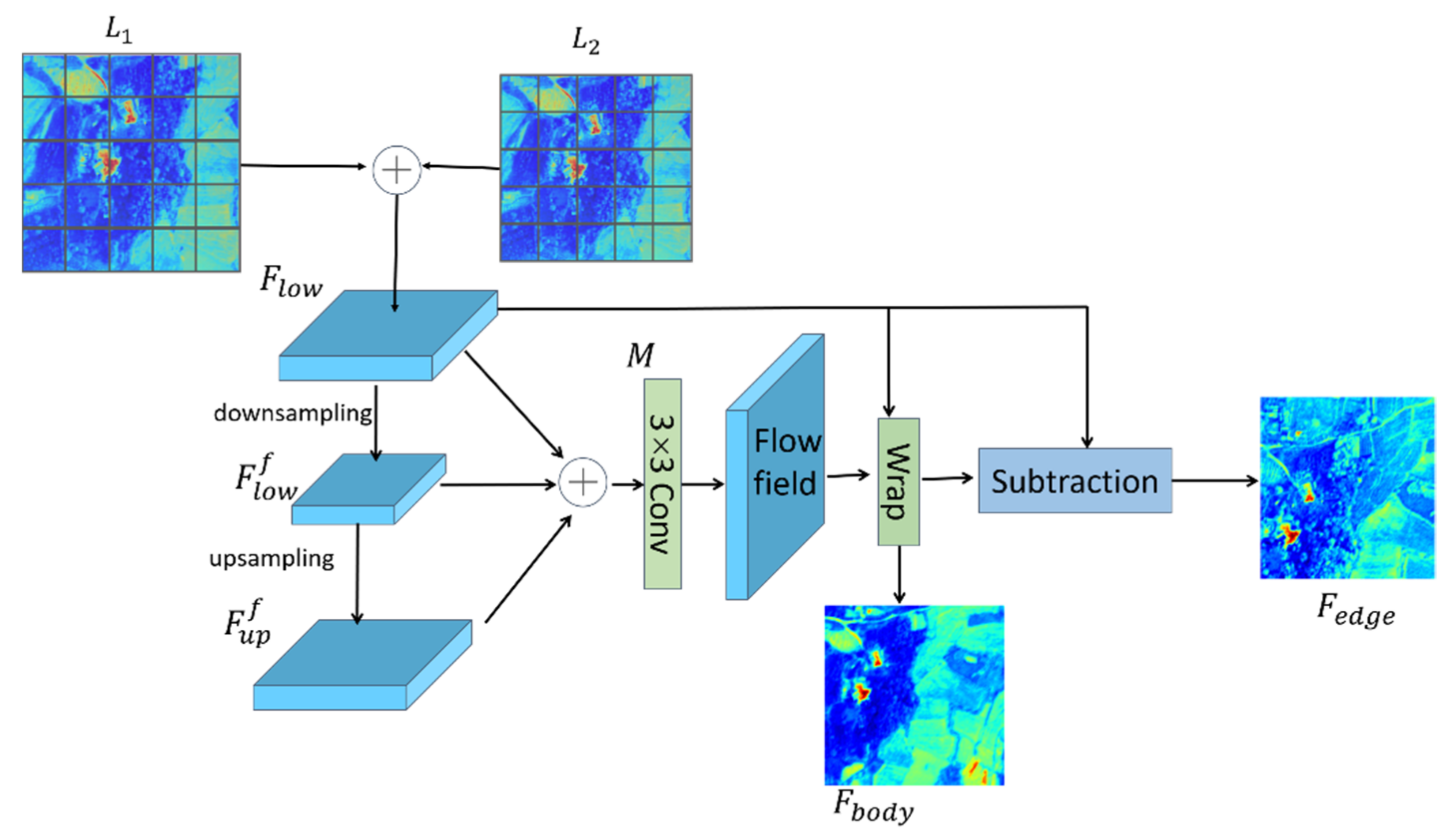
2.2. Boundary and Body Separation Module (BBS)

We propose a boundary body separation module (BBS) that separates boundary features from body features using high and low frequency information [36]. The BBS decomposes the semantic segmentation low-level features into two parts: boundary features$F_{edge}$ and body features $F_{body}$. From the decomposition of the high-resolution low-level features into body features and edge features, the main structure of the BBS is shown in Figure 4. From Figure 4, we can learn that after feature fusion of feature map$L_{1 }$and feature map $L_2$, the boundary features and body features are then obtained by the BBS. The boundary features$F_{edge}$ get clearer boundary information, while the information boundary of the feature map obtained in the body features $F_{body}$ can retain most of the global information.

Two parts are required to obtain the body features: flow field generation and feature distortion. The body feature refers to the part of the flow that points to the center of the feature $F_{low}$ throughout the flow field generation process. In order to create a flow that mainly points to the center of the object, we focused on the features of the central part of the object.

The low-frequency feature map $F_{low}^f$ is first generated by downsampling the feature $F_{low}$and then the low-frequency feature map $F_{low}^f$ is upsampled to the same size $F_{up}^f$. The three feature maps ($F_{low}$, $F_{low}^f$, $F_{up}^f$) are concatenated and compressed by using the convolutional layer to obtain the prediction map $M$.

The feature warping is performed to reassign a new coordinate position $p_i+M\left(p_i\right)$ to each pixel point at position $p_i$ on the original standard image. Each pixel point $p_x$ in the body features $F_{body}$can be approximated by a micro-bilinear sampling mechanism [37]. The adopted microscopic bilinear sampling mechanism is formulated as follows:

$$F_{body}\left(p_x\right)={\displaystyle \sum }_{n\in NP\left(p_i\right)}{m}_n{F}_{low}\left(n\right)$$

(1)

$NP$ represents the set of 4 nearest neighbor pixel points of $p_i$, and $m_n$ is the bilinear kernel weight on the distorted space grid, computed by predicting the prediction map$M$. After the wrapping process, the edge features $F_{edge}$ are acquired through the subtraction of the feature map $F_{low}$from the acquired body features $F_{body}$.

$$F_{edge}=F_{low}-F_{body}$$

(2)

2.3. Boundary Detail Enhancement Module (BDE)

The BDE is used to refine the boundary information of edge features in different level features. The module mainly contains two parts: module a and module b. First, module BDE (a) is applied to the refinement of features $L_3,L_4$, and then BDE (b) is applied to integrate the feature information of different level features. The detail enhancement module is mainly composed of cross-convolution [38]. The cross-convolution is different from the ordinary convolution, which obtains more feature information by crossing from two directions, horizontal and vertical, in a different order, as shown in Figure 5a. After sending the feature map to the cross-convolution, the corresponding two convolution kernels perform feature extraction according to the vertical and horizontal directions, and the arrows in the Figure 5a indicate the gradient direction of the pixels.

The structure of cross-convolution is shown in Figure 5b and consists of two asymmetric vertical filters $k_{1\times t}$ and $k_{t\times 1}$ with a receptive field size of $1\times t$ for filter $k_{1\times t}$ and $t\times 1$ for filter $k_{t\times 1}$. Assuming the cross-convolution input features $F_{in}^{cro}$, the output features $F_{out}^{cro}$ consists of the convolution of the input features $F_{in}^{cro}$ and the vertical filter plus the deviation $b$. The formula is calculated as follows:

$$F_{out}^{cro}=k_{1\times t}\otimes F_{in}^{cro}+k_{t\times 1}\otimes F_{in}^{cro}+b$$

(3)

Instead of extracting features in one direction, cross-convolution focuses on extracting features crosswise in the vertical and horizontal directions, compared to normal convolution layers. This parallel design mode preserves more details and also focuses more on boundary information.

As shown in Figure 3, BDE (a) consists of two cross-convolutions, with the feature map first passing through the first cross-convolution, followed by the RELU layer, then the second cross-convolution, and finally the feature normalization (F-Norm) [39].

F-Norm is a feature normalization method starting from the feature channel. Assuming that different channels contain different information, F-Norm designs different channels to process the information in parallel, thus reducing the parameters and computational complexity. This parallel processing of normalized features can also effectively prevent the missing details caused by cross-channel information fusion. The F-Norm is calculated as follows:

$$f_{out}^j=\left(g_j\times f_{in}^j+b_j\right)+f_{in}^j$$

(4)

where $j$ is the channel index,$f_{out}^j$ is the output feature channels,$f_{in}^j$ is the input channels.$g$ is a convolutional kernel, and $b$ stands for bias. In order to retain more contextual feature information at higher levels, the pre- and post-normalization features were appended to the output.

Feature map $L_3$ and feature map $L_4$ were feature fused into one feature map after going through BDE (a) operation. After that, the feature map was upsampled to get feature map $F_{high}^{\prime }$ sized as the $L_3$. The feature fused feature map is feature enhanced using module BDE (b) to obtain feature map $P_2$. BDE (b) mainly consists of a combination of cross-convolution and channel attention mechanism [40], which can ensure that the fused feature maps can achieve the integration of global and local information. We average the channel dimension and convert it to one dimension for visualization. Figure 6a shows the original image, Figure 6b shows the visualization of features after BDE(a) operation, and Figure 6c visualization of features after BDE(a) operation and BDE(b) operation. As shown in Figure 6, the boundary information of the feature map becomes more distinct after BDE (b).

The feature map $F_{high}^{\prime }$ is the same size as the features $F_{low}$. After connecting $F_{high}^{\prime }$ and $F_{edge}$, the feature map $F_r$ is calculated as follows:

$$F_r=F_{edge}+F_{high}^{\prime }$$

(5)

The obtained feature map $F_r$contains more boundary information. $F_r$needs to interact with the boundary subject information with the body feature map $F_{body}$, which is extracted from the feature, $F_{low}$, to obtain the prediction map $P_1$.

2.4. The Module for Interaction between Boundary Information and Body Information (IBBM)

We propose IBBM for the interaction of boundary features and body features, as shown in Figure 7, which is used to fuse features from the feature map $F_r$ and the body features $F_{body}$ extracted from the low-level features. There are various ways of information interaction, but the main objective is to enable more efficient feature fusion. We design the function to calculate the interaction information as follows:

$$E\left(x_1,x_2\right)=\alpha \times x_1+\beta \times x_2$$

(6)

where $\alpha$ and $\beta$ are the learnable scalar weights of the input body information $x_1$ and boundary information $x_2$.

As shown in Figure 7, we first interacted with the information of body features $F_{body}$and boundary features $F_r$, and generated feature maps $F_{body}^u$ by nearest-neighbor interpolation of the feature maps obtained from the interaction. The specific calculation formula is as follows:

$$E\left(F_{body},F_r\right)=\alpha \times F_{body}+\beta \times F_r$$

(7)

We performed nearest-neighbor interpolation on the boundary features to obtain the features $F_r^u$. After that we interacted with the information of body features $F_{body}^u$ and boundary features $F_r^u$. The specific calculation formula is as follows:

$$E\left(F_r^u,F_{body}^u\right)={\alpha }^{\prime }\times F_r^u+{\beta }^{\prime }\times F_{body}^u$$

(8)

where${\alpha }^{\prime }$and ${\beta }^{\prime }$ are the learnable scalar weights of the input body information $F_{body}^u$ and boundary information $F_r^u$. When interacting with boundary information and subject information, each information interaction is done according to the corresponding position pixel and then find the neighboring pixels in the same position for interaction. After implementing the boundaries and body information interact with each other between the two feature maps, the feature map $P_1$ is generated.

2.5. Cross-Detail Module

We designed a cross-detail module, which can fully guarantee the interaction of contextual and global information while achieving the preservation of more detailed and local information. The cross-detail module is mainly composed of the Cross-Attention [33,41] and the improved MLP. The cross-detail module is shown in Figure 8a.

The module obtains the high-level features $P_1,P_2$and category information from the backbone network $cl{s}_1,cl{s}_3$, where $cl{s}_i=\left[c_i^1,c_i^2,\dots ,c_i^{Nc}\right]\in R^{Nc\times D}$, $Nc$ is the count of classes, $c_i^k$ is the $k$-th class of stage $i$. The features $P_1,P_2$corresponds to tokens $z_1,z_2$. These tokens are transformed into corresponding keys $k$, values $v$ by linear change, and $cl{s}_1,cl{s}_3$ into queries $q$ by linear change. The main operations of the Cross-Attention layer are as follows:

$$\begin{gathered} k=z_i{W}_k,v=z_i{W}_v,q=cl{s}_i{W}_q \\ CA=softmax(\frac{q{k}^T}{\sqrt{\frac{D}{h}}})v+cl{s}_i \end{gathered}$$

(9)

It is noted that $W_k,W_v,W_q\in {ℝ}^{D\times \left(\mathrm{D}/\mathrm{h}\right)}$ are learnable parameters,$D$ stands for embedding dimension, and $h$ stands for the count of heads. The Cross-Attention operation is mainly to obtain more context and is efficiently computational. The module is mainly used to find the relevant information needed and integrate it into the existing features. In this paper, cross-detail module is mainly used to search for more contextual information while maintaining the class information.

The MLP structure is shown in Figure 8b, which consists of two fully connected layers, and an intermediate layer of activation function GELU. FC layer is used in the conventional feedforward layer implements pixel-by-pixel propagation, which results in the inability to learn cross token information. The cross-convolution changes the original fully connected layer with a single information interaction by extracting information from two directions in parallel. We set up the detail branch to the MLP layer, and the detail branch consists of two cross-convolutions. The design MLP layer is calculated as follows:

$$\begin{gathered} x_1=FC\left(x_{in},{\theta }_1\right) \\ {x}_{out}=FC\left(\sigma \left(x_1+CS\left(x_1\right)\right),{\theta }_2\right) \end{gathered}$$

(10)

where $x_{in }$ denotes the input features, $x_{out}$ denotes the output features, $CS$ denotes the added cross-convolution module branches, ${\theta }_1$ and ${\theta }_2$ denote the optional parameters, $FC$ means full connectiVity layer, σ represents the active layer. The output feature map$P_3$ is obtained from $P_1$ with the cross-detail module, and the output feature map$P_4$ is obtained from $P_2$ with the cross- detail module. The final output prediction map is obtained by connecting the $P_3$ and upsampling $P_4$ of the hierarchical refinement of boundary features.

3. Results and Discussion

3.1. Datasets

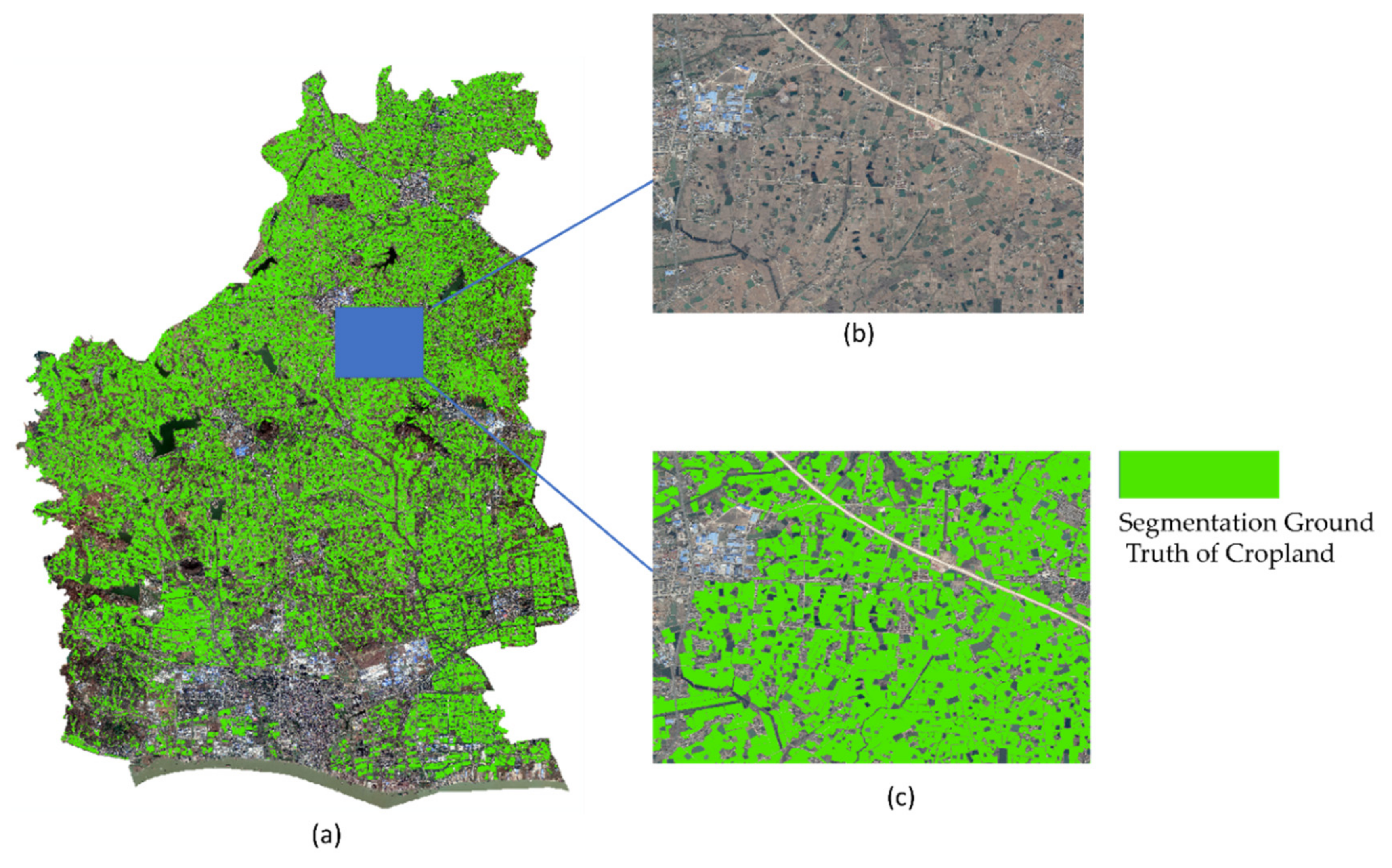
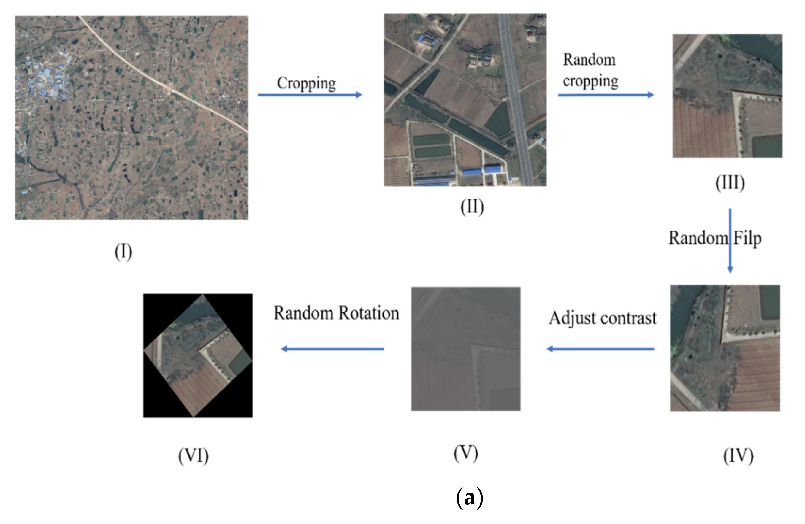
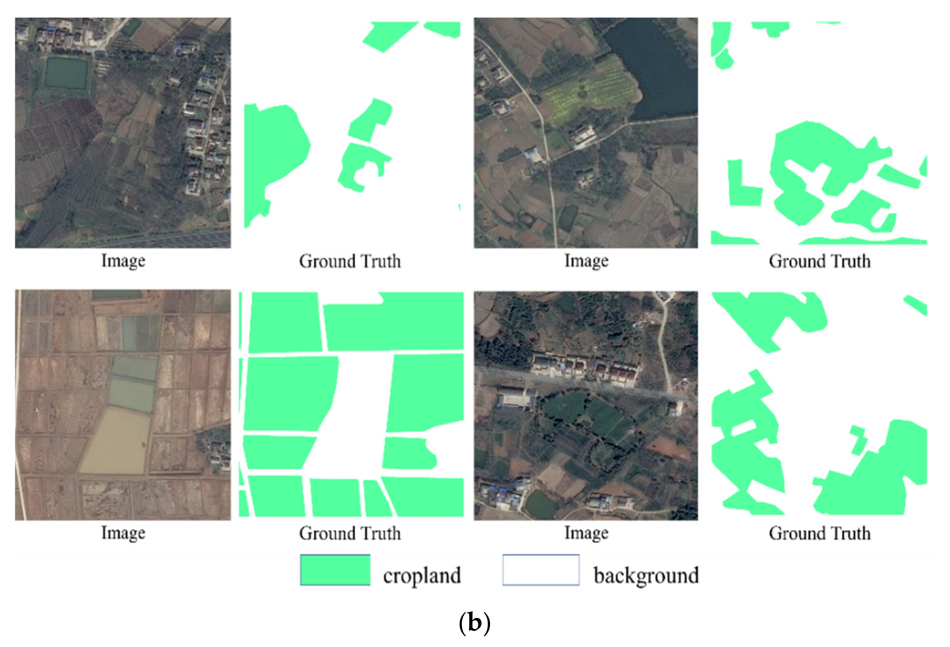
3.1.1. Agriculture Dataset

The dataset used Google Maps as the source of high-resolution images with a resolution of 0.3 m. The Agriculture dataset is mainly from the remote sensing images of Yizheng City, Yangzhou City, as shown in Figure 9. Most of the obtained images are cropland subdivisions, and the whole dataset is divided into two categories: Cropland and Background. We perform precise semantic segmentation labeling on the obtained remote sensing images. As shown in Figure 10a, we crop the images, and the cropped image size was 1456 × 1456, with 1280 images in total. After that, we crop the image to a random size of 325 × 325 for training purposes. We randomly select random copping, adjust contrast and random rotation for data enhancement.

Figure 10b contains some images and the label of the Agriculture dataset, where the label in green represents the cropland and the label in white represents the background area.

3.1.2. DeepGlobe Dataset

This public dataset is a total of 80 satellite images with a spatial resolution of 0.5 m and a pixel size of 2448 × 2448 for each image in the dataset. The DeepGlobe dataset focuses on the geographic types of rural areas and needs to be partitioned into seven classes. The DeepGlobe dataset, derived from an open challenge, is satellite imagery with a resolution of 0.5 m, with a focus on rural areas. Overall, 56.76% of the pixel classes in the dataset are agricultural land. The dataset is divided into a high number of categories and a dense distribution of categories, containing a large amount of mountainous woodland. The total area of the dataset is equivalent to 1716.9 km². In this paper, we discard the “Unknown” category and split the sample into six classes, namely Urban, Agriculture, Rangeland, Forest, Water, and Barren. We divided the dataset according to the method proposed in the literature [29], with 455 training sets, 207 validation sets, and 142 test sets. We crop the image to a random size of 512 × 512 for training purposes. We randomly select random copping, adjust contrast, and random rotation for data enhancement.

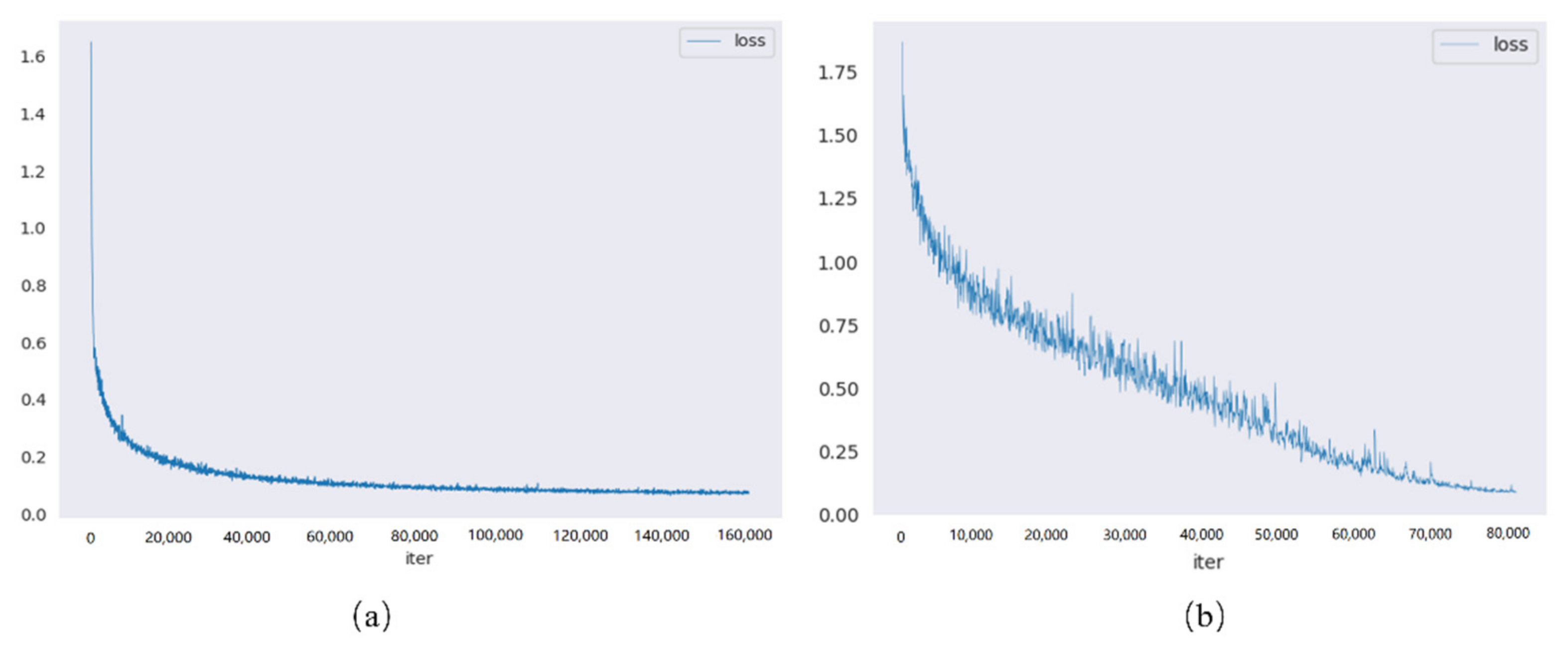
3.2. Implementation Details

The learning rate size for the initial training is set to 8 and a “poly” learning rate strategy is used. The initial learning rate was set to 1e-3 and the power to 0.9. We use AdamW with a weight decay of 1e-2. For the DeepGlobe dataset, we trained 80K iterations. For the Agriculture dataset, we trained 160 K iterations. All experiments are performed on a Tesla V100. We employed the overall accuracy (OA) and the mean Intersection over Union (mIoU) to evaluate model performance.

$$\mathrm{OA}=\frac{{{\displaystyle \sum }}_{k=1}^{N}T{P}_k}{{{\displaystyle \sum }}_{k=1}^{N}T{P}_k+F{P}_k+T{N}_k+F{N}_k}$$

(11)

$$mIoU=\frac{1}{N}{\displaystyle \sum }_{k=1}^N\frac{T{P}_k}{T{P}_k+F{P}_k+F{N}_k}$$

(12)

where $T{P}_k$ is the true positive for class $k$, $F{P}_k$ is the false positive for class $k$, $T{N}_k$ is the true negative for class $k$, and $F{N}_k$ is the false negative for class $k$. Figure 11 shows the loss reduction curve of the two datasets, respectively. The loss curves all fall slowly and smoothly, with the end result being convergence.

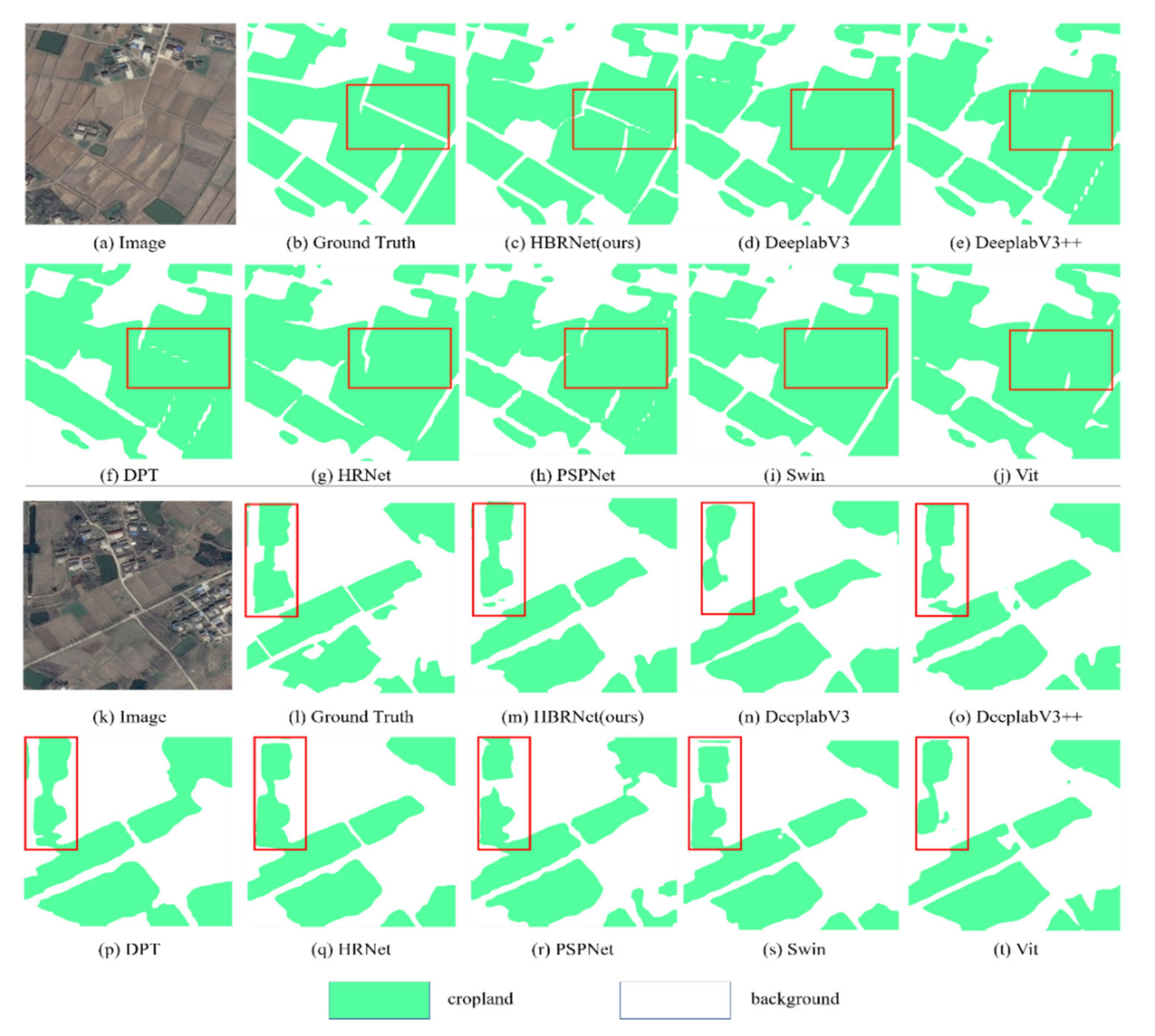
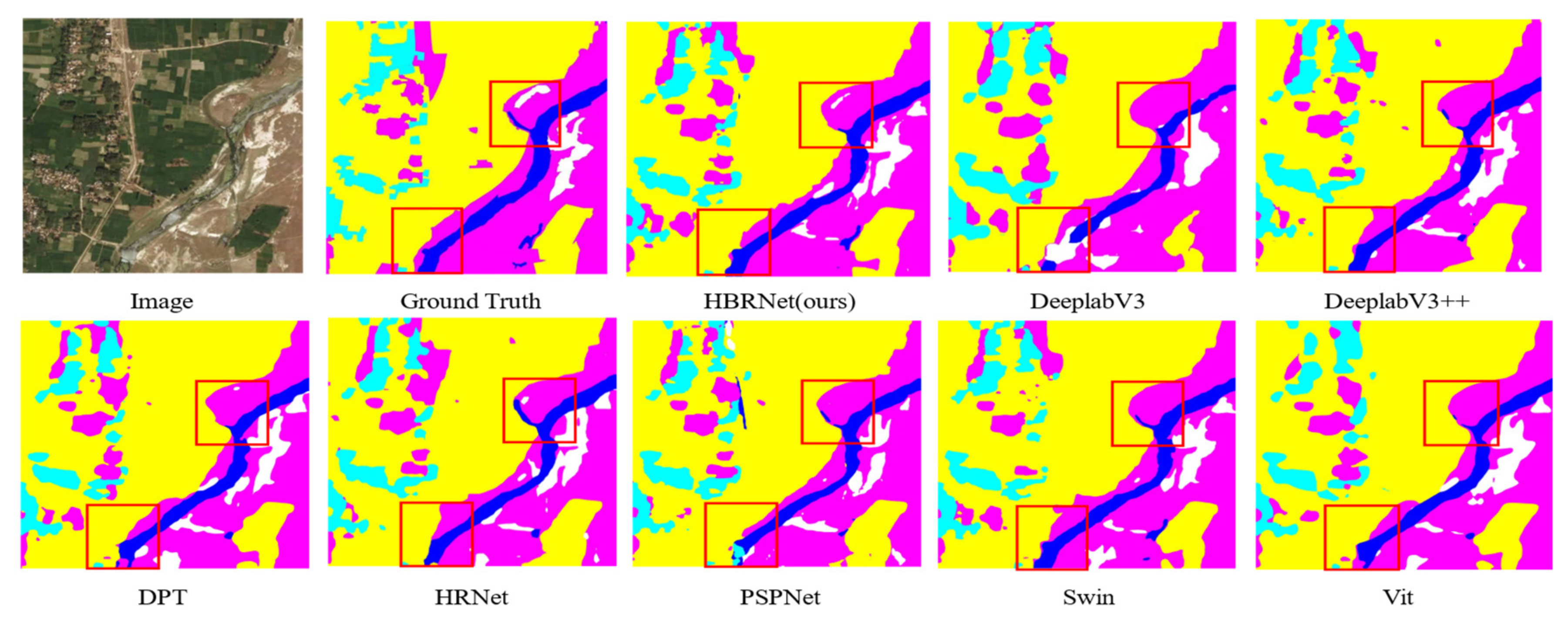
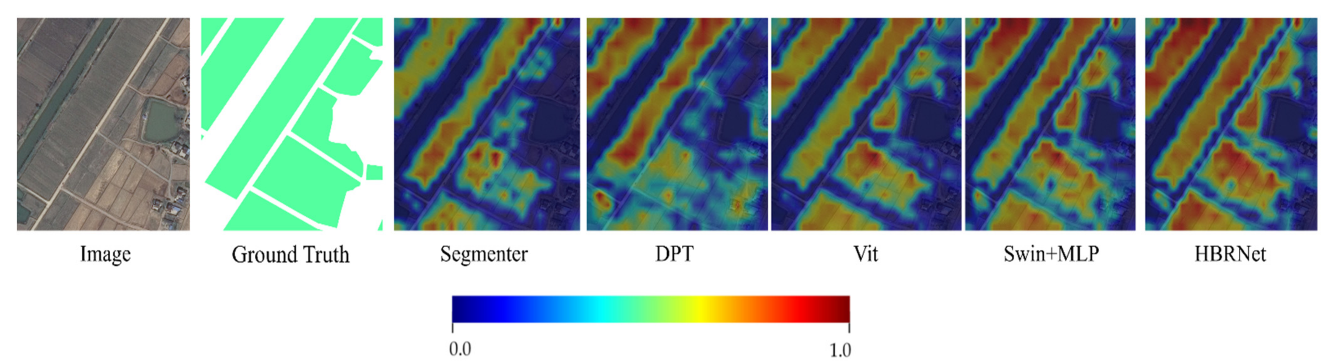
3.3. Semantic Segmentation Results and Analysis

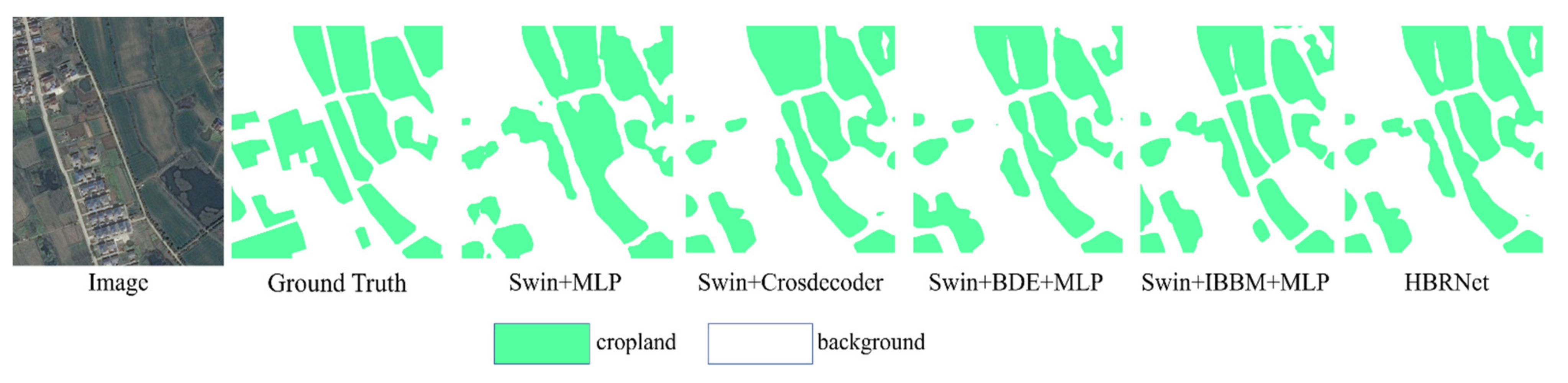
The existing semantic segmentation algorithms HRNet [42], PSPNet [17], DeeplabV3 [43], DeeplabV3+ [44], DPT [45], Vit [13], IsaNet [46], Unet [47], ApcNet [48], SegFormer [49], and Segmenter [50] have achieved excellent performance in semantic segmentation. In this paper, we compare HBRNet with the above semantic segmentation networks in the same network framework and setup. HRNet effectively improves the accuracy by the network structure that keep the high resolution of the features. DeepLabV3 and PSPNet are also multi-layered structures with multi-scale feature fusion modules, which also achieve effective improvement in semantic segmentation. Vit is the breakthrough in the application of transformer mechanism to image semantic segmentation, which can obtain contextual information well.

Table 1. Results on the Agriculture dataset test set (the result with the highest value is bolded). We employed the overall accuracy (OA), Intersection over Union (IoU) of Per Category and the mean Intersection over Union (mIoU) to evaluate model performance.

Method	Backbone	IoU Per Category (%)		mIoU (%)	OA
		CropLand	Background
HRNet	W32	81.99	70.92	76.46	87.49
PSPNet	ResNet50	82.70	71.52	77.11	87.94
IsaNet	ResNet50	82.66	71.40	77.03	87.90
UNet + FCN	UNet-S5	79.08	69.00	74.08	85.74
ApcNet	ResNet50	82.55	71.38	76.97	87.84
DeeplabV3	ResNet50	81.73	70.84	76.28	87.34
Deeplab V3+	ResNet50	82.58	71.60	76.87	87.82
Swin-MLP	Swin-T	83.70	73.20	78.45	88.72
SegFormer	MIT-B0	82.89	72.86	77.92	88.32
Segmenter-Mask	Vit-T_16	83.47	72.93	78.20	88.56
DPT	Vit-b16	83.62	72.17	78.17	88.60
Vit-upernet	Vit-b16	83.60	73.12	78.36	88.66
HBRNet	Swin-T	84.59	74.64	79.61	89.40

shows the experimental performance on the Agriculture dataset. HBRNet achieves the highest mIoU of 79.61% and OA of 89.4% when the backbone is Swin. Our proposed method HBRNet improves the mIoU of CropLand by 1.18% on this dataset of Agriculture compared to Vit network with attention mechanism.

Table 2. Results on the DeepGlobe dataset test set (the result with the highest value is bolded). We employed the overall accuracy (OA), Intersection over Union (IoU) of Per Category and the mean Intersection over Union (mIoU) to evaluate model performance.

Method	Backbone	IoU Per Category (%)						mIoU (%)	OA
		Urban	Agriculture	Range	Forest	Water	Barren
HRNet	W32	72.57	88.08	36.02	80.64	82.57	62.59	70.41	88.03
PSPNet	ResNet50	73.28	88.66	38.25	81.38	83.36	64.10	71.50	88.51
IsaNet	ResNet50	78.05	88.09	34.30	78.55	78.28	68.39	70.94	88.47
UNet + FCN	UNet-S5	72.73	86.97	33.15	79.99	81.64	57.46	68.66	86.94
ApcNet	ResNet50	72.42	89.02	41.58	83.55	83.45	61.08	71.85	88.75
DeeplabV3	ResNet50	71.99	88.57	35.27	81.46	81.65	63.64	70.43	88.19
Deeplab V3+	ResNet50	72.93	88.55	34.98	81.27	84.05	61.99	70.63	88.24
Swin- MLP	Swin-T	75.00	89.85	44.32	83.74	85.44	66.35	74.12	89.60
SegFormer	MIT-B0	74.66	89.22	42.99	84.16	83.47	63.84	73.06	89.25
Segmenter	Vit-T16	74.68	89.41	43.11	83.16	84.10	66.50	73.49	89.32
DPT	Vit-b16	73.22	88.80	40.91	82.98	82.60	65.96	72.29	88.73
Vit- upernet	Vit-b16	72.55	89.19	44.48	83.02	80.10	66.96	72.72	88.92
HBRNet	Swin-T	76.28	90.37	47.93	84.36	84.67	67.37	75.15	90.16

shows the experimental results on the DeepGlobe dataset, where our proposed method has the highest mIoU of 75.15% and OA of 90.16%. HBRNet improves the mIoU metric by 6.73% and the OA metric by 2.42% compared to HRNet, a high-resolution semantic segmentation network with convolution as the main structure. As shown in Table 1 and Table 2, the head of Vit is upernet [51]. Compared with the existing hierarchical structure networks (such as PSPNet and DeepLabV3), our proposed HBRNet applies attention mechanism to obtain more contextual information. The boundary information is enhanced by fusion of hierarchical information, which effectively improves the accuracy of segmentation.

The results visualized on the Agriculture dataset are shown in Figure 12, which illustrates that the present method achieves more significant fine feature representation results than other methods. The results of the image segmentation on the DeepGlobe dataset are displayed in Figure 13. From Figure 12, we can observe that HBRNet improves the accuracy of the cropland extraction. The distribution of labels in the red box is worth being focused on, where HBRNet performs with greater attention to details in the extraction of the cropland compared to the other algorithms. First, consider the top half of Figure 12. Figure 12a shows the original image, Figure 12b shows the correctly segmented label information, Figure 12c shows the output of our method, and the remainder show the output of the comparison experiment. From the red box in Figure 12, we can see that there is a white border across the correctly segmented labels. This border is partially segmented by our algorithm, but other algorithms such as DeepLabV3, HRNet, and PSPNet do not identify it, while the DPT algorithm identifies a few white dots. Next, consider the bottom half of Figure 12. Similar to the top half, Figure 12k shows the original image, Figure 12i shows the correctly segmented label information, Figure 12m shows the output of our method, and the remainder shows the output of the comparison experiment. We can observe the segmentation in the red box. For correctly segmented label information, the lower part of the green label inside the box does not meet the other green. In other words, there is a boundary. We find that several segmentation results in the fourth row do not identify this boundary well, and in the third row the DeeplabV3 image and the DeepLabV3 recognition results differ from the label information at the boundary by a large result. Although our method does not fully identify the boundary, it achieves more promising results compared to other algorithms.

We chose two images as examples, and from Figure 13, we can observe that HBRNet network achieves satisfactory performance in both overall segmentation of multiple classes of objects and segmentation of small objects. In particular, for cropland segmentation with some detailed information, HBRNet segmented cropland has more delicate boundaries compared to other algorithms.

To further illustrate the effectiveness of our network, we generate the probability heat map of cropland in the final layers of Segmenter, DPT, Vit, Swin, and HBRNet. As shown in Figure 14, the features are normalized between (0,1). The degree of distinctness of an area of cropland corresponds to the shade of color—the more red areas and the darker the color, the more likely it is to be cropped. We can see from the heat map that our algorithm is more aware of contextual information and is better able to extract ploughing features.

3.4. Ablation Study

We performed ablation experiments on the Agriculture dataset and the DeepGlobe dataset, and the experimental results are shown in

Table 3. The ablation experiments on the Agriculture dataset evaluated by mIoU (%) and OA (%) about the methods. We employed the overall accuracy (OA), Intersection over Union (IoU) of Per Category and the mean Intersection over Union (mIoU) to evaluate model performance.

Method	IoU Per Category (%)		mIoU (%)	OA
	CropLand	Background
Swin + mlp	83.7	73.2	78.45	88.72
Swin + CDD	83.78	73.67	78.73	88.85
Swin + BDE + mlp	84.03	73.85	78.94	88.99
Swin + IBBM + mlp	83.81	73.91	78.86	88.9
Swin + BDE + IBBM + CDD	84.59	74.64	79.61	89.4

and

Table 4. The ablation experiments on the DeepGlobe dataset evaluated by mIoU (%) and OA (%) about the methopds. We employed the overall accuracy (OA), Intersection over Union (IoU) of Per Category and the mean Intersection over Union (mIoU) to evaluate model performance.

Method	IoU Per Category (%)						mIoU (%)	OA
	Urban	Agriculture	Range	Forest	Water	Barren
Swin + mlp	75.00	89.85	44.32	83.74	85.44	66.35	74.12	89.60
Swin + CDD	74.54	90.18	47.24	84.18	85.62	67.84	74.93	89.95
Swin + BDE + mlp	75.45	90.27	45.30	82.72	86.96	67.73	74.74	89.76
Swin + IBBM + mlp	75.33	90.08	46.89	83.79	86.44	67.57	75.02	89.85
Swin + BDE + IBBM + CDD	76.18	90.37	47.93	84.36	84.67	67.37	75.15	90.16

, respectively. As shown in Table 3 and Table 4, “swin” indicates Swin-T as the backbone. Specifically, four sets of experiments were implemented to evaluate the performance of the Cross Detail Module (CDD), the Boundary Detail Enhancement (BDE), and the Interaction Between Boundary Features and Body Features Module (IBBM).

Details of the implementation of these four sets of experiments are as follows. In experiment 1, Swin-T is the backbone and multi-layer perceptron (MLP) is the head. In experiment 2, Swin-T is the backbone and CDD is the head. The cross-detail module is added as head to compare whether the cross-detail module we design is helpful to improve the segmentation performance. We use CDD for the output features, respectively, and get two output prediction maps. The final prediction is obtained by fusing the features of the two output prediction maps. In experiment 3, we use Swin-T as the backbone and MLP as the head. We add BDE for high-level features and use CDD for low-level features. After we use BDE for high-level features, we use CDD. The output features of different features after CDD are fused to obtain the final output prediction map. In experiment 4, we use Swin-T as the backbone and MLP as the head. The specific details are as follows. Firstly, BBS is used for low-level features to obtain boundary features and body features. Then, the features obtained by feature fusion of boundary features and high-level features are used as the input of IBBM. Another input feature of IBBM is the body features. From the results of the ablation experiment, we can reveal that Swin + CDD + BDE + IBBM improve the performance of the backbone method dramatically. From the observation of the experimental results, we can conclude that all four main modules in HBRNet are effective in advancing cropland extraction.

In order to further reveal the role of CDD, BDE, and IBBM, we visualize the results on the Agriculture and DeepGlobe datasets after adding CDD, BDE, and IBBM on backbone in Figure 15 and Figure 16. As shown in the third, fourth, and fifth columns of Figure 15, these methods lack the processing of boundary information. Comparing the sixth column in Figure 15, HBRNet contains enhanced boundary features. From the Figures, we can observe that each module plays a positive role in the acquisition of boundary and contextual information.

4. Conclusions

Accurately extracted cropland helps to achieve precision agriculture and promotes the maintenance of grain security. In this paper, we used semantic segmentation algorithm to extract cropland from high-resolution remote sensing images. We propose a hierarchical boundary enhancement semantic segmentation method (HBRNet), which tackles the problem of boundary information degradation during cropland extraction. In addressing the issue of cropland extraction, we have made three key findings. Firstly, HBRNet uses the boundary body separation module (BBS) to extract the boundary information. This approach focuses more on the high-resolution feature maps and thus is more beneficial for extracting cropland. Secondly, in order to obtain a feature map with more details, the module for interaction between boundary information and body information (IBBM) is proposed. Thirdly, we conducted experiments on a cropland dataset containing large-scale cropland in Yizheng City. Experiments on the Agriculture dataset and the DeepGlobe dataset show that our algorithm is effective in compensating for poor boundary information on cropland extraction. Compared with some algorithms, HBRNet achieves the best results in cropland extraction, achieving 84.59% in IoU on Agriculture dataset. In future work, we will consider the fusion of multiple sources of data for the extraction of cropland, including earth surface temperature images, hyperspectral images, multispectral images, nearing infrared images, etc.

References

1. Huang, J.; Weng, L.; Chen, B.; Xia, M. DFFAN: Dual Function Feature Aggregation Network for Semantic Segmentation of Land Cover. ISPRS Int. J. Geo-Inf. 2021, 10, 125. [Google Scholar] [CrossRef]
2. Zhang, H.; Peng, Q. PSO and K-means-based semantic segmentation toward agricultural products. Future Gener. Comput. Syst. 2022, 126, 82–87. [Google Scholar] [CrossRef]
3. Nzabarinda, V.; Bao, A.; Xu, W.; Uwamahoro, S.; Huang, X.; Gao, Z.; Umugwaneza, A.; Kayumba, P.M.; Maniraho, A.P.; Jiang, Z. Impact of cropland development intensity and expansion on natural vegetation in different African countries. Ecol. Inform. 2021, 64, 101359. [Google Scholar] [CrossRef]
4. Liu, J.; Wang, D.; Maeda, E.E.; Pellikka, P.K.E.; Heiskanen, J. Mapping Cropland Burned Area in Northeastern China by Integrating Landsat Time Series and Multi-Harmonic Model. Remote Sens. 2021, 13, 5131. [Google Scholar] [CrossRef]
5. Copenhaver, K.; Hamada, Y.; Mueller, S.; Dunn, J.B. Examining the Characteristics of the Cropland Data Layer in the Context of Estimating Land Cover Change. ISPRS Int. J. Geo-Inf. 2021, 10, 281. [Google Scholar] [CrossRef]
6. Chen, Q.; Cao, W.; Shang, J.; Liu, J.; Liu, X. Superpixel-Based Cropland Classification of SAR Image with Statistical Texture and Polarization Features. IEEE Geosci. Remote Sens. Lett. 2022, 19, 1–5. [Google Scholar] [CrossRef]
7. Sun, Y.; Qin, Q.; Ren, H.; Zhang, Y. Decameter Cropland LAI/FPAR Estimation From Sentinel-2 Imagery Using Google Earth Engine. IEEE Trans. Geosci. Remote Sens. 2022, 60, 1–14. [Google Scholar] [CrossRef]
8. Chen, J.; Wang, H.; Guo, Y.; Sun, G.; Zhang, Y.; Deng, M. Strengthen the Feature Distinguishability of Geo-Object Details in the Semantic Segmentation of High-Resolution Remote Sensing Images. IEEE J. Sel. Top. Appl. Earth Obs. Remote Sens. 2021, 14, 2327–2340. [Google Scholar] [CrossRef]
9. He, X.; Zhou, Y.; Zhao, J.; Zhang, M.; Yao, R.; Liu, B.; Li, H. Semantic Segmentation of Remote-Sensing Images Based on Multiscale Feature Fusion and Attention Refinement. IEEE Geosci. Remote Sens. Lett. 2022, 19, 1–5. [Google Scholar] [CrossRef]
10. Wei, H.; Xu, X.; Ou, N.; Zhang, X.; Dai, Y. DEANet: Dual Encoder with Attention Network for Semantic Segmentation of Remote Sensing Imagery. Remote. Sens. 2021, 13, 3900. [Google Scholar] [CrossRef]
11. Zheng, S.; Lu, J.; Zhao, H.; Zhu, X.; Luo, Z.; Wang, Y.; Fu, Y.; Feng, J.; Xiang, T.; Torr, P.H.S.; et al. Rethinking Semantic Segmentation from a Sequence-to-Sequence Perspective with Transformers. In Proceedings of the IEEE/CVF Conference on Computer Vision and Pattern Recognition(CVPR), Virtual, 19–25 June 2021; pp. 6881–6890. [Google Scholar]
12. Yuan, Y.; Chen, X.; Wang, J. Object-Contextual Representations for Semantic Segmentation. In Proceedings of the European Conference on Computer Vision(ECCV), Glasgow, UK, 23–28 August 2020; pp. 173–190. [Google Scholar]
13. Yuan, Y.; Fu, R.; Huang, L.; Lin, W.; Zhang, C.; Chen, X.; Wang, J. HRFormer: High-Resolution Transformer for Dense Prediction. arXiv 2021, arXiv:2110.09408. [Google Scholar]
14. Ganesan, R.; Raajini, X.M.; Nayyar, A.; Padmanaban, S.; Hossain, E.; Ertas, A.H. BOLD: Bio-Inspired Optimized Leader Election for Multiple Drones. Sensors 2020, 20, 3134. [Google Scholar] [CrossRef]
15. Wei, Z.; Youqiang, S.; He, H.; Haotian, P.; Jiajia, S.; Po, Y. Pest Region Detection in Complex Backgrounds via Contextual Information and Multi-Scale Mixed Attention Mechanism. Agriculture 2022, 12, 1104. [Google Scholar]
16. Zhao, H.; Shi, J.; Qi, X.; Wang, X.; Jia, J. Pyramid Scene Parsing Network. In Proceedings of the IEEE Conference on Computer Vision and Pattern Recognition (CVPR), Honolulu, HI, USA, 21–26 July 2017; pp. 6230–6239. [Google Scholar]
17. Liu, M.; Yin, H. Efficient pyramid context encoding and feature embedding for semantic segmentation. Image Vis. Comput. 2021, 111, 104195. [Google Scholar] [CrossRef]
18. Bousselham, W.; Thibault, G.; Pagano, L.; Machireddy, A.; Gray, J.; Chang, Y.H.; Song, X. Efficient Self-Ensemble Framework for Semantic Segmentation. arXiv 2021, arXiv:2111.13280. [Google Scholar]
19. Wang, L.; Li, R.; Duan, C.; Zhang, C.; Meng, X.; Fang, S. A Novel Transformer based Semantic Segmentation Scheme for Fine-Resolution Remote Sensing Images. IEEE Geosci. Remote Sens. Lett. 2022, 19, 1–5. [Google Scholar] [CrossRef]
20. Peng, C.; Ma, J. Semantic segmentation using stride spatial pyramid pooling and dual attention decoder. Pattern Recognit. 2020, 107, 107498. [Google Scholar] [CrossRef]
21. Liu, Z.; Lin, Y.; Cao, Y.; Hu, H.; Wei, Y.; Zhang, Z.; Lin, S.; Guo, B. Swin Transformer: Hierarchical Vision Transformer using Shifted Windows. In Proceedings of the IEEE/CVF International Conference on Computer Vision(ICCV), Montreal, QC, Canada, 10–17 October 2021; pp. 9992–10002. [Google Scholar]
22. Wang, L.; Li, R.; Wang, D.; Duan, C.; Wang, T.; Meng, X. Transformer meets convolution: A bilateral awareness network for semantic segmentation of very fine resolution urban scene images. Remote Sens. 2021, 13, 3065. [Google Scholar] [CrossRef]
23. Chong, Y.; Chen, X.; Pan, S. Context Union Edge Network for Semantic Segmentation of Small-Scale Objects in Very High Resolution Remote Sensing Images. IEEE Geosci. Remote Sens. Lett. 2022, 19, 10–14. [Google Scholar] [CrossRef]
24. Pan, S.; Tao, Y.; Nie, C.; Chong, Y. PEGNet: Progressive Edge Guidance Network for Semantic Segmentation of Remote Sensing Images. IEEE Geosci. Remote Sens. Lett. 2021, 18, 637–641. [Google Scholar] [CrossRef]
25. Li, H.; Qiu, K.; Chen, L.; Mei, X.; Hong, L.; Tao, C. SCAttNet: Semantic Segmentation Network with Spatial and Channel Attention Mechanism for High-Resolution Remote Sensing Images. IEEE Geosci. Remote Sens. Lett. 2021, 18, 905–909. [Google Scholar] [CrossRef]
26. Ghandorh, H.; Boulila, W.; Masood, S.; Koubaa, A.; Ahmed, F.; Ahmad, J. Semantic Segmentation and Edge Detection—Approach to Road Detection in Very High Resolution Satellite Images. Remote Sens. 2022, 14, 613. [Google Scholar] [CrossRef]
27. Li, Q.; Yang, W.; Liu, W.; Yu, Y.; He, S. From Contexts to Locality: Ultra-high Resolution Image Segmentation via Locality-aware Contextual Correlation. In Proceedings of the IEEE/CVF International Conference on Computer Vision, Montreal, QC, Canada, 10–17 October 2021; pp. 7232–7241. [Google Scholar]
28. Huynh, C.; Tran, A.; Luu, K.; Hoai, M. Progressive Semantic Segmentation. In Proceedings of the IEEE Conference on Computer Vision and Pattern Recognition(CVPR), Virtual, 19–25 June 2021; pp. 16755–16764. [Google Scholar]
29. Zhu, L.; Ji, D.; Zhu, S.; Gan, W.; Wu, W.; Yan, J. Learning statistical texture for semantic segmentation. In Proceedings of the IEEE Conference on Computer Vision and Pattern Recognition, Virtual, 19–25 June 2021; pp. 12532–12541. [Google Scholar]
30. Chen, B.; Xia, M.; Huang, J. MFANet: A Multi-Level Feature Aggregation Network for Semantic Segmentation of Land Cover. Remote. Sens. 2021, 13, 731. [Google Scholar] [CrossRef]
31. Padmanaban, S.; Daya, F.J.L.; Blaabjerg, F.; Wheeler, P.W.; Szcześniak, P.; Oleschuk, V.; Ertas, A.H. Wavelet-fuzzy speed indirect field oriented controller for three-phase AC motor drive—Investigation and implementation. Eng. Sci. Technol. Int. J. 2016, 19, 1099–1107. [Google Scholar] [CrossRef] [Green Version]
32. Padmanaban, S.; Daya, F.J.L.; Blaabjerg, F.; Mir-Nasiri, N.; Ertas, A.H. Numerical implementation of wavelet and fuzzy transform IFOC for three-phase induction motor. Eng. Sci. Technol. Int. J. 2016, 19, 96–100. [Google Scholar] [CrossRef] [Green Version]
33. Wang, J.; Zheng, Z.; Ma, A.; Lu, X.; Zhong, Y. LoveDA: A Remote Sensing Land-Cover Dataset for Domain Adaptive Semantic Segmentation. In Proceedings of the Neural Information Processing Systems Track on Datasets and Benchmarks, Virtual, 6–14 December 2021; pp. 1–16. [Google Scholar]
34. Demir, I.; Koperski, K.; Lindenbaum, D.; Pang, G.; Huang, J.; Basu, S.; Hughes, F.; Tuia, D.; Raska, R. DeepGlobe 2018: A challenge to parse the earth through satellite images. In Proceedings of the IEEE Computer Society Conference on Computer Vision and Pattern Recognition Workshops, Salt Lake City, UT, USA, 18–22 June 2018; pp. 172–181. [Google Scholar]
35. Li, X.; Li, X.; Zhang, L.; Cheng, G.; Shi, J.; Lin, Z.; Tan, S.; Tong, Y. Improving Semantic Segmentation via Decoupled Body and Edge Supervision. In Proceedings of the European Conference on Computer Vision, Glasgow, UK, 23–28 August 2020; pp. 435–452. [Google Scholar]
36. Zhu, X.; Xiong, Y.; Dai, J.; Yuan, L.; Wei, Y. Deep feature flow for video recognition. In Proceedings of the IEEE Conference on Computer Vision and Pattern Recognition, Honolulu, HI, USA, 21–26 July 2017; pp. 4141–4150. [Google Scholar]
37. Liu, Y.; Jia, Q.; Fan, X.; Wang, S.; Ma, S.; Gao, W. Cross-SRN: Structure-Preserving Super-Resolution Network with Cross Convolution. IEEE Trans. Circuits Syst. Video Technol. 2021, 32, 4927–4939. [Google Scholar] [CrossRef]
38. Liu, Y.; Wang, S.; Zhang, J.; Wang, S.; Ma, S.; Gao, W. Iterative Network for Image Super-Resolution. IEEE Trans. Multimed. 2021, 24, 2259–2272. [Google Scholar] [CrossRef]
39. Hu, J.; Shen, L.; Albanie, S.; Sun, G.; Wu, E. Squeeze-and-Excitation Networks. IEEE Trans. Pattern Anal. Mach. Intell. 2020, 42, 2011–2023. [Google Scholar] [CrossRef] [Green Version]
40. Chen, C.-F.R.; Fan, Q.; Panda, R. CrossViT: Cross-Attention Multi-Scale Vision Transformer for Image Classification. In Proceedings of the IEEE/CVF International Conference on Computer Vision, Montreal, QC, Canada, 11–17 October 2021; pp. 347–356. [Google Scholar]
41. Wang, J.; Sun, K.; Cheng, T.; Jiang, B.; Deng, C.; Zhao, Y.; Liu, D.; Mu, Y.; Tan, M.; Wang, X.; et al. Deep High-Resolution Representation Learning for Visual Recognition. IEEE Trans. Pattern Anal. Mach. Intell. 2020, 43, 3349–3364. [Google Scholar] [CrossRef] [Green Version]
42. Chen, L.-C.; Papandreou, G.; Schroff, F.; Adam, H. Rethinking Atrous Convolution for Semantic Image Segmentation. arXiv 2017, arXiv:1706.05587. [Google Scholar]
43. Kim, T.H.; Sajjadi, M.S.M.; Hirsch, M.; Sch, B. Encoder-Decoder with Atrous Separable Convolution for Semantic. In Proceedings of the European Conference on Computer Vision, Munich, Germany, 8–14 September 2018; pp. 111–127. [Google Scholar]
44. Ranftl, R.; Bochkovskiy, A.; Koltun, V. Vision Transformers for Dense Prediction. In Proceedings of the IEEE/CVF International Conference on Computer Vision, Montreal, QC, Canada, 10–17 October 2021; pp. 12159–12168. [Google Scholar]
45. Huang, L.; Yuan, Y.; Guo, J.; Zhang, C.; Chen, X.; Wang, J. Interlaced Sparse Self-Attention for Semantic Segmentation. arXiv 2019, arXiv:1907.12273. [Google Scholar]
46. Ronneberger, O.; Fischer, P.; Brox, T. U-Net: Convolutional Networks for Biomedical Image Segmentation. arXiv 2015, arXiv:1505.04597. [Google Scholar]
47. He, J.; Deng, Z.; Zhou, L.; Wang, Y.; Qiao, Y. Adaptive Pyramid Context Network for Semantic Segmentation. In Proceedings of the IEEE/CVF Conference on Computer Vision and Pattern Recognition, Long Beach, CA, USA, 16–20 June 2019; pp. 7519–7528. [Google Scholar]
48. Xie, E.; Wang, W.; Yu, Z.; Anandkumar, A.; Alvarez, J.M.; Luo, P. SegFormer: Simple and Efficient Design for Semantic Segmentation with Transformers. In Proceedings of the Annual Conference on Neural Information Processing Systems, Virtual, 6–14 December 2021; pp. 12077–12090. [Google Scholar]
49. Strudel, R.; Pinel, R.G.; Laptev, I.; Schmid, C. Segmenter: Transformer for Semantic Segmentation. In Proceedings of the IEEE/CVF International Conference on Computer Vision, Montreal, QC, Canada, 10–17 October 2021; pp. 7242–7252. [Google Scholar]
50. Fan, M.; Lai, S.; Huang, J.; Wei, X.; Chai, Z.; Luo, J.; Wei, X. Rethinking BiSeNet for Real-Time Semantic Segmentation. In Proceedings of the IEEE Conference on Computer Vision and Pattern Recognition, Virtual, 19–25 June 2021; pp. 9716–9725. [Google Scholar]
51. Xiao, T.; Liu, Y.; Zhou, B.; Jiang, Y.; Sun, J. Unified Perceptual Parsing for Scene Understanding. In Proceedings of the European Conference on Computer Vision, Munich, Germany, 8–14 September 2018; pp. 432–448. [Google Scholar]
Figure 1. Three boundary refinement structures. (a) The refinement of high-level features. (b) The refinement of low-level features. (c) Module with hierarchical refinement (ours). “RM” indicates refinement module.
Agriculture 12 01284 g001
Figure 2. Two transformer blocks in Swin transformer in succession. MLP stands for multi-layer perceptron.
Agriculture 12 01284 g002
Figure 3. Overall structure of HBRNet. The figure shows the main modules for processing high-level features and low-level features. After inputting the original map, two level features are output through a hierarchical structure, and the feature map is processed separately. The output features of Swin Transformer from the first stage to the fourth stage as L 1 , L 2 , L 3 , L 4 . F b o d y stands for body features. F e d g e stands for boundary features. F h i g h represents the features obtained after the BDE (a) for the high-level features. F r represents the features generated by the combination of boundary features and F h i g h . P 1 represents the features generated after the low-level feature processing. P 1 represents the features generated after the low-level features processing.   P 2 represents the features generated after the high-level features processing. F-Norm stands for feature normalization. ReLU stands for rectified linear unit. Cross-Conv stands for cross-convolution.
Agriculture 12 01284 g003
Figure 4. Main structure of boundary and body separation. We upsampled features L 2 and combined it with features L 1 to obtain low-level features F l o w . F l o w f is obtained by downsampling with F l o w . F u p f is obtained by upsampling with F l o w f . F e d g e represents the edge features. F b o d y represents the body features.
Agriculture 12 01284 g004
Figure 5. (a) Cross-convolution obtains more feature information by taking more information from both horizontal and vertical directions. (b) The structure of cross-convolution. F i n c r o represents cross-convolution input features and F o u t c r o represents cross-convolution out features. 1 × t Conv stands for convolution kernel size of 1 × t . t × 1 Conv stands for convolution kernel size of t × 1 .
Agriculture 12 01284 g005
Figure 6. (a) The original image, (b) Visualization of features after BDE (a) operation, (c) Visualization of features after BDE (a) operation and BDE (b) operation.
Agriculture 12 01284 g006
Figure 7. The structure of the interaction between boundary features and body features. α ,   β , α ,   and β are the learnable scalar weights of the input body information. The boundary features F r and the body features F b o d y have the same size. The boundary features F r u and the body features F b o d y u have the same size.
Agriculture 12 01284 g007
Figure 8. (a) The structure of cross-detail module, FC stands for fully-connected, Norm stands for Layer Normalization, and k means keys, v means values, and q means queries. (b) The structure of multi-layer perceptron (MLP). GELU stands for Gaussian Error Linear Unit, which is an activation function. F-Norm stands for feature normalization. ReLU stands for rectified linear unit.
Agriculture 12 01284 g008
Figure 9. Large area of cropland extraction results in Yizheng City, Yangzhou City, Jiangsu Province. (a) Cropland results extracted from high-resolution remote sensing images, (b) true color image in the blue box in (a), (c) ground truth of semantically segmented cropland in (b).
Agriculture 12 01284 g009
Figure 10. (a) The main steps of data processing. The figure shows several data enhancement methods, including random copping, adjust contrast, and random rotation. These methods are random selection in order. (b) Original images of some of the cropland and the labeling of the cropland areas.
Agriculture 12 01284 g010aAgriculture 12 01284 g010b
Figure 11. Training plots for the cropland extraction network in the dataset: (a) training decreasing loss curves in the Agriculture dataset, (b) training decreasing loss curves in the DeepGlobe dataset.
Agriculture 12 01284 g011
Figure 12. Visualization of results on the Agriculture dataset. The green represents the distribution of cropland and the white is the background. We can focus on comparisons of the details in the red boxes when observing the figure of the experimental results.
Agriculture 12 01284 g012
Figure 13. Visualization of results on the DeepGlobe dataset. We have marked some detailed information in the experimental results section with red boxes, and by comparing this information we can see which algorithms achieved better results.
Agriculture 12 01284 g013aAgriculture 12 01284 g013b
Figure 14. The probability heat map of cropland. The redder the red represents the greater likelihood that the section is arable land and indicates that the experimental results are closer to the true results.
Agriculture 12 01284 g014
Figure 15. Visualization of the results on the Agriculture dataset after adding different modules on Swin-T.
Agriculture 12 01284 g015
Figure 16. Visualization of the results on the DeepGlobe dataset after adding different modules on Swin-T.
Agriculture 12 01284 g016