
Energy Saving Performance of Agricultural Tractor Equipped with Mechanic-Electronic-Hydraulic Powertrain System


Abstract
:1. Introduction
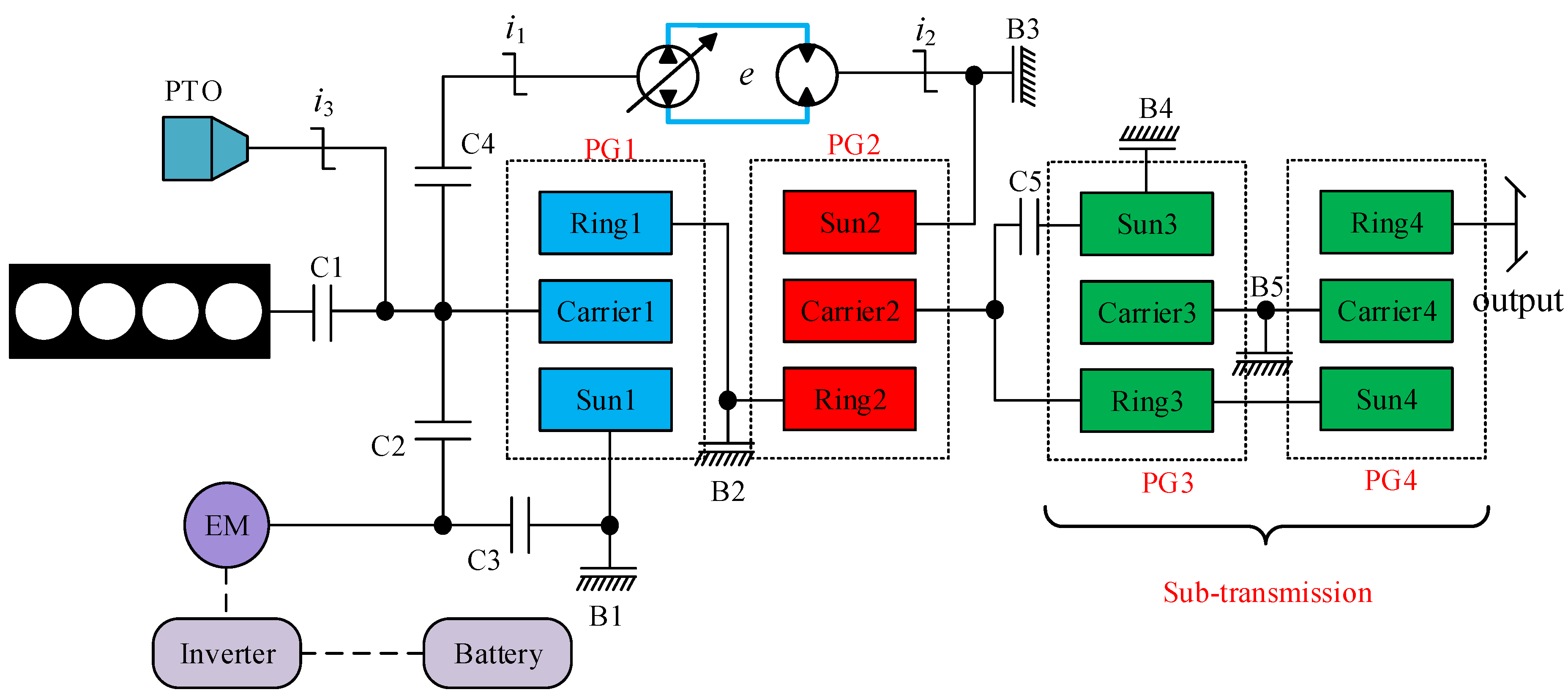
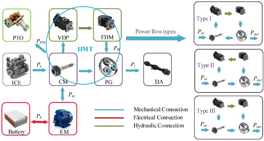
2. Principle of Powertrain Configuration
2.1. Driving Mode Analysis
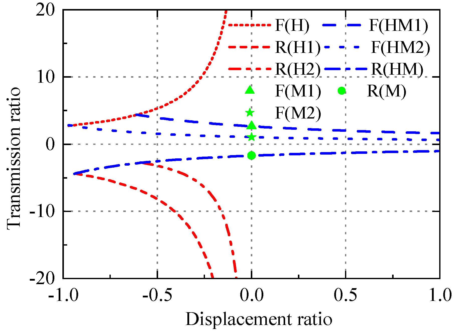
2.2. Transmission Mode Analysis
3. Powertrain Modeling
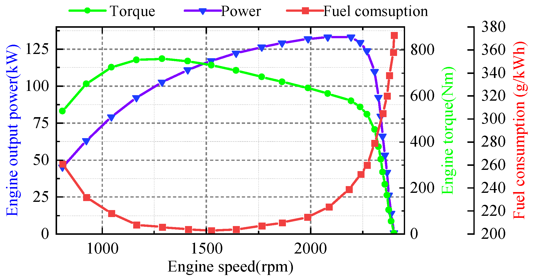
3.1. Engine Model
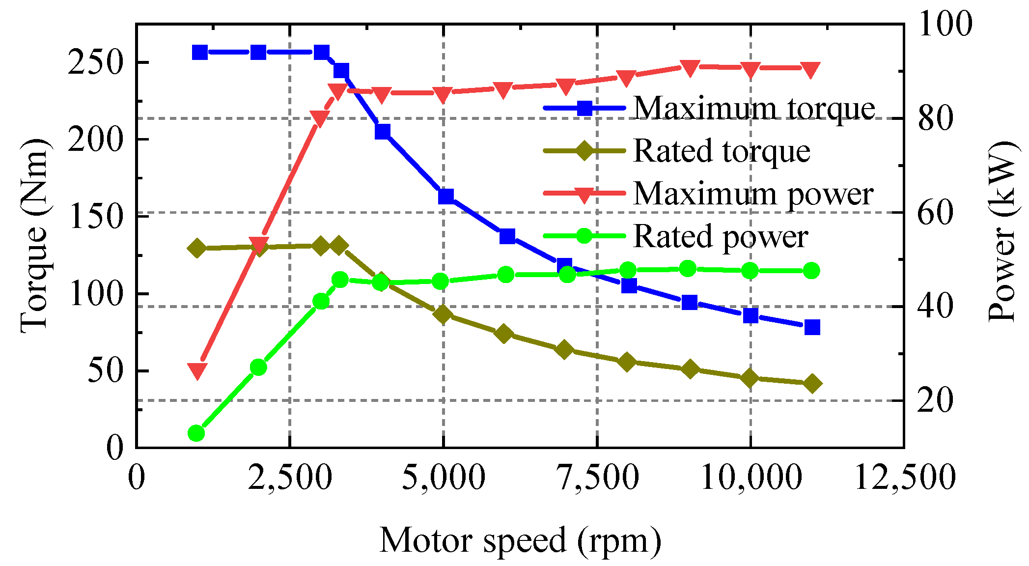
3.2. Motor Model
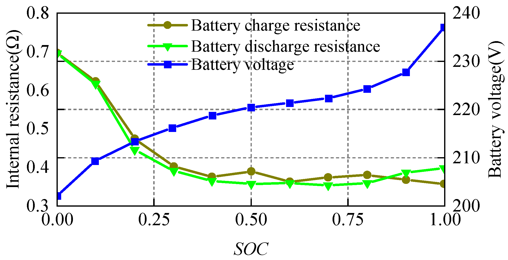
3.3. Battery Model
3.4. Transmission Model
3.5. Tractor Model
4. Tractor Control Strategy
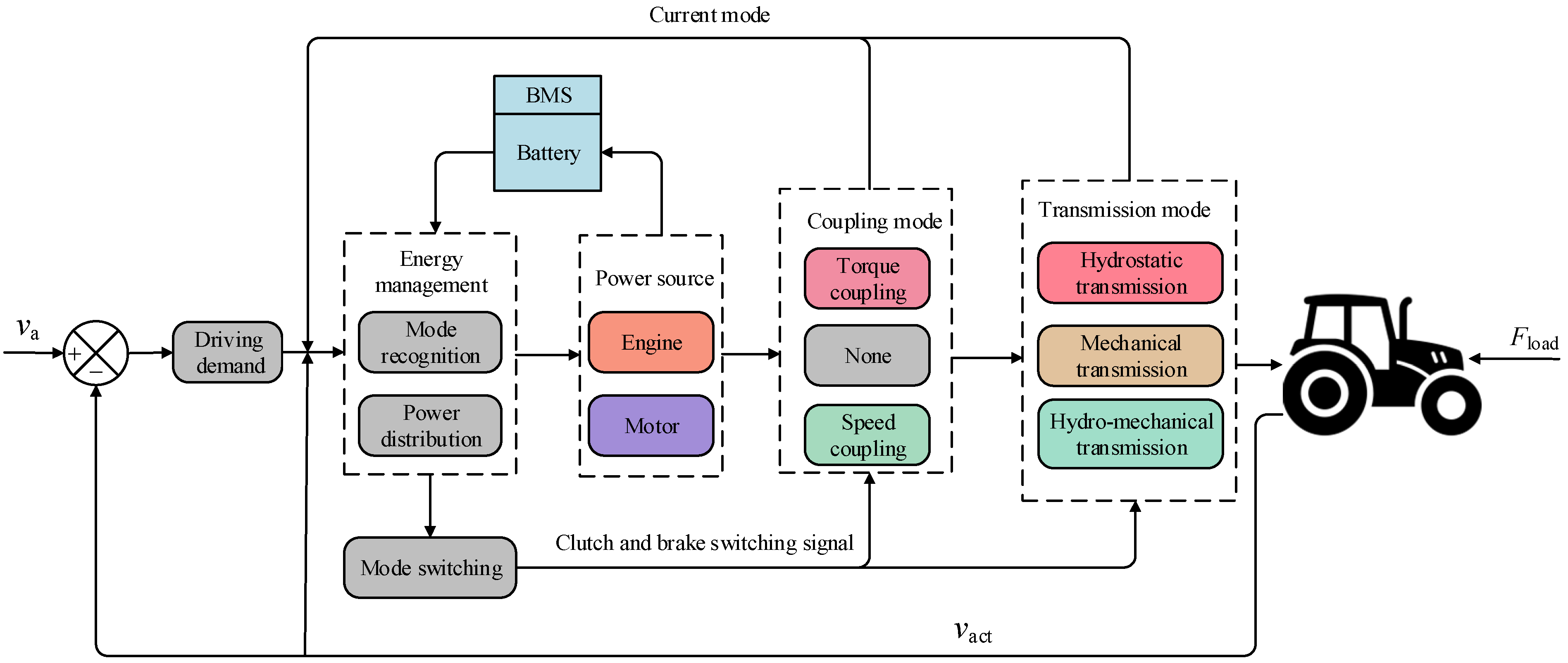
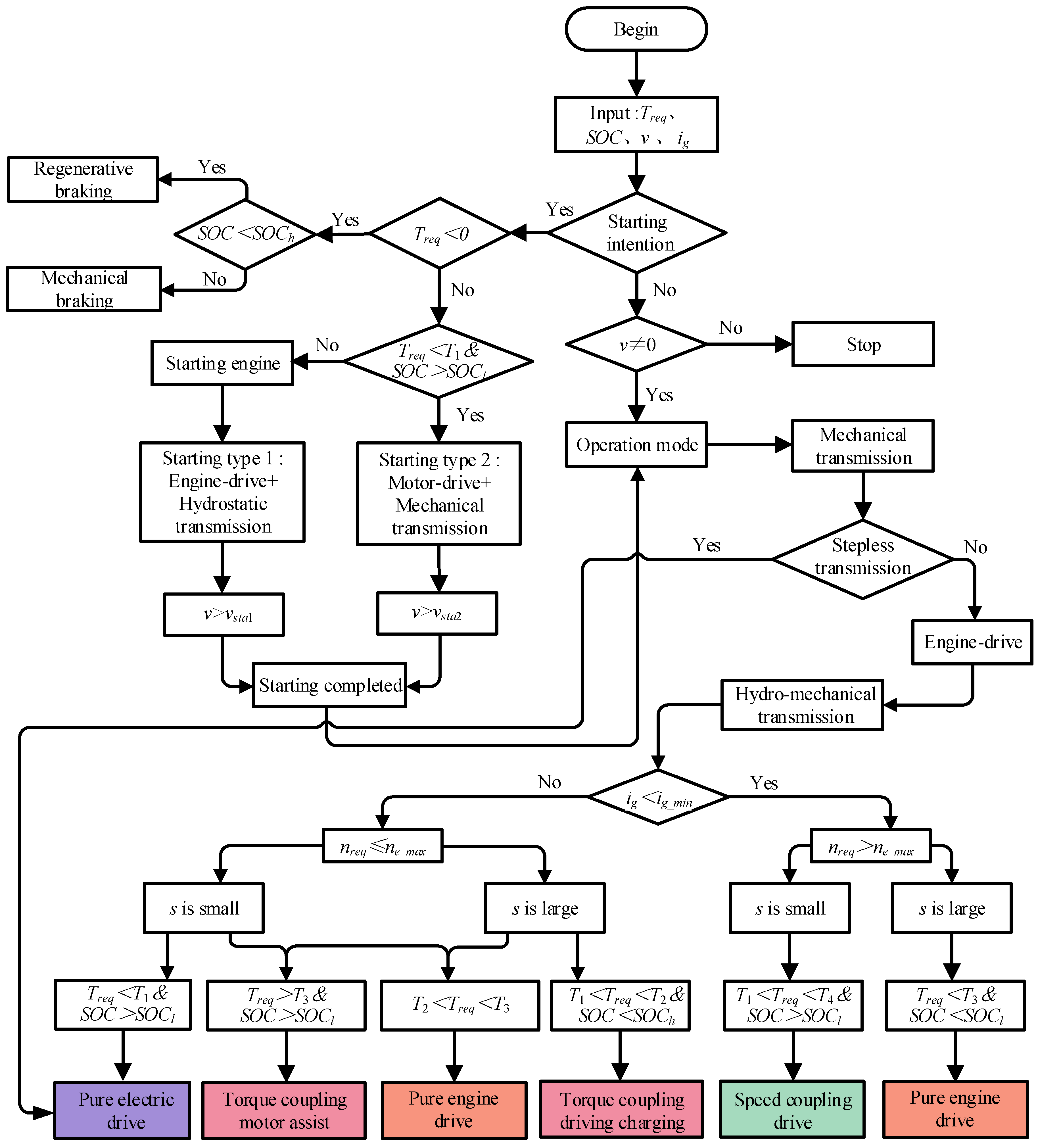
4.1. Overall Control Strategy
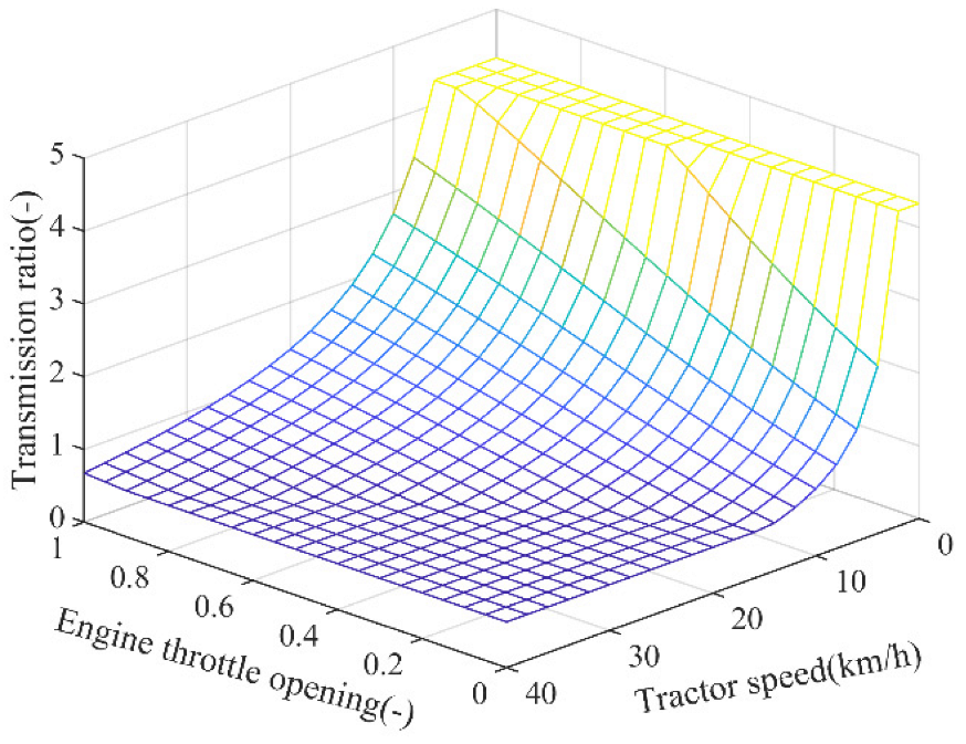
4.2. HMT Transmission Ratio Control Strategy
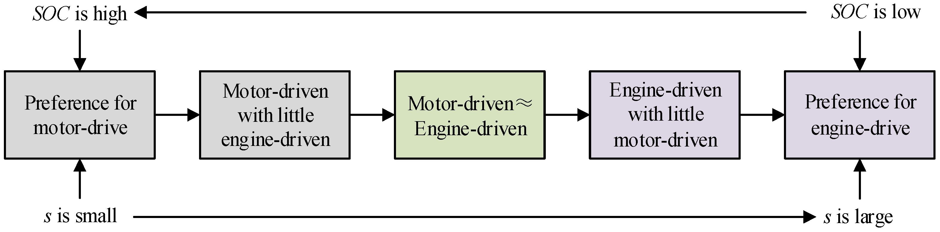
4.3. Mode Division of Rule-Based
4.4. Optimization Strategy with Minimal Equivalent Fuel Consumption
5. Simulation and Experiment
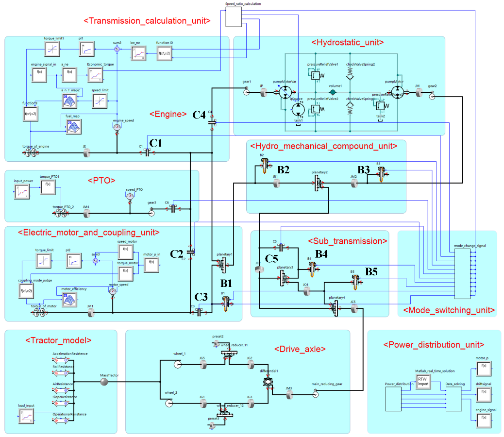
5.1. Simulation Modeling
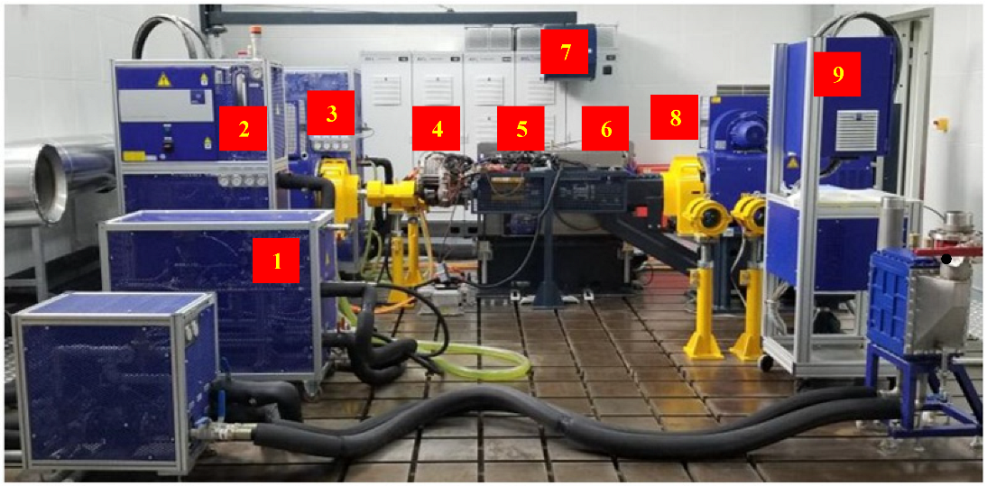
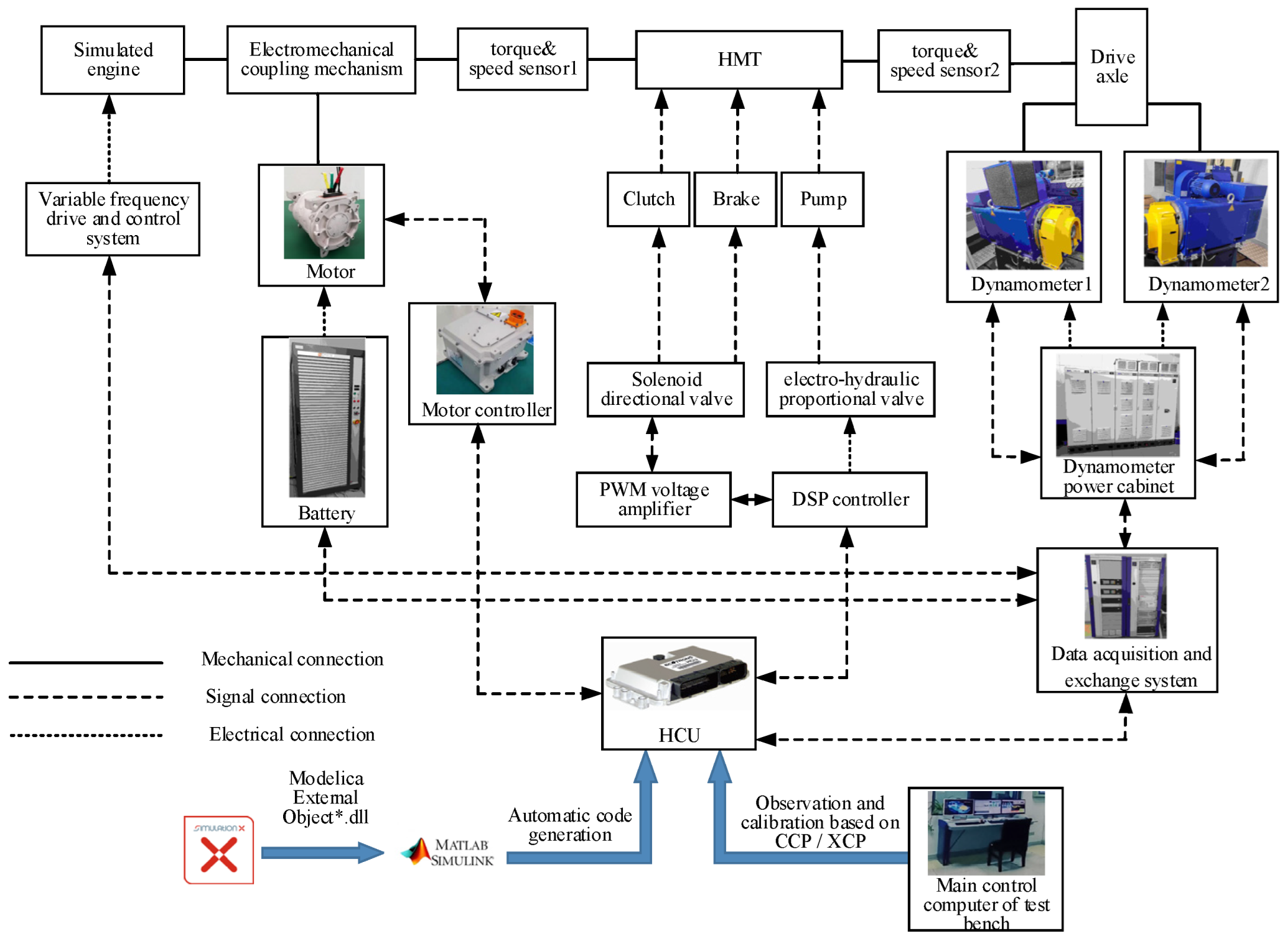
5.2. Test Bench and Principle
5.3. Simulation and Test of Tractor Operation
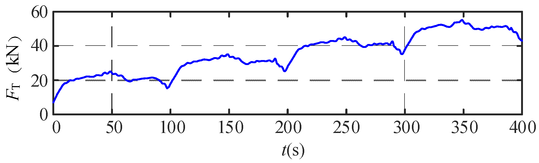
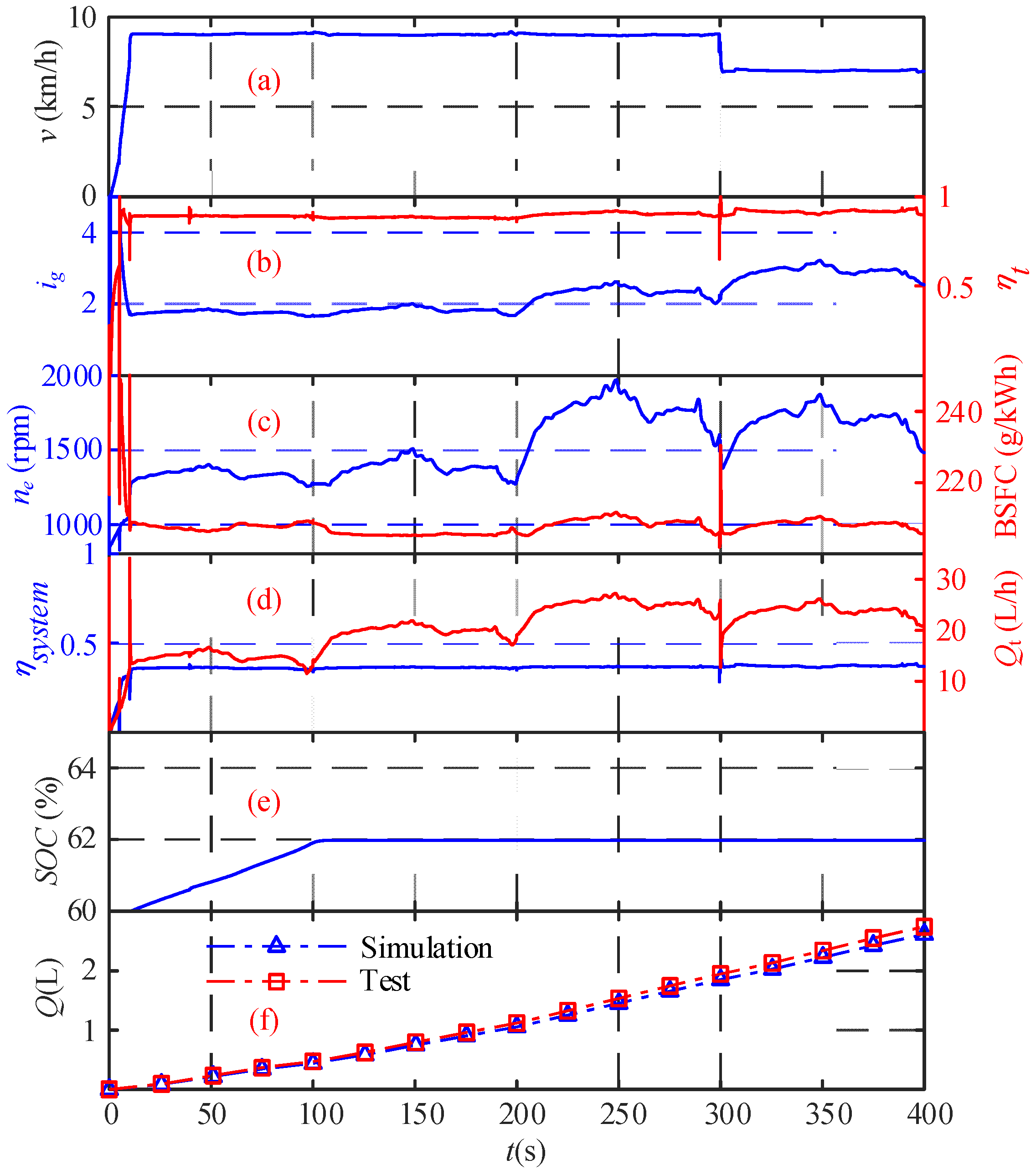
5.3.1. Ploughing Analysis
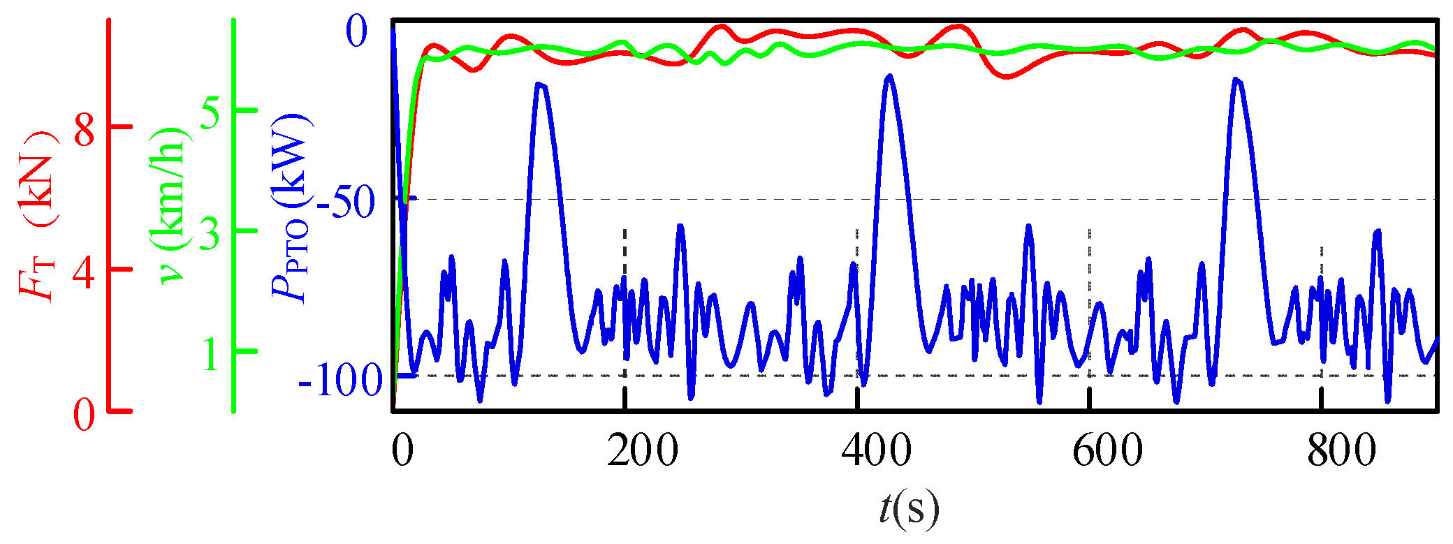
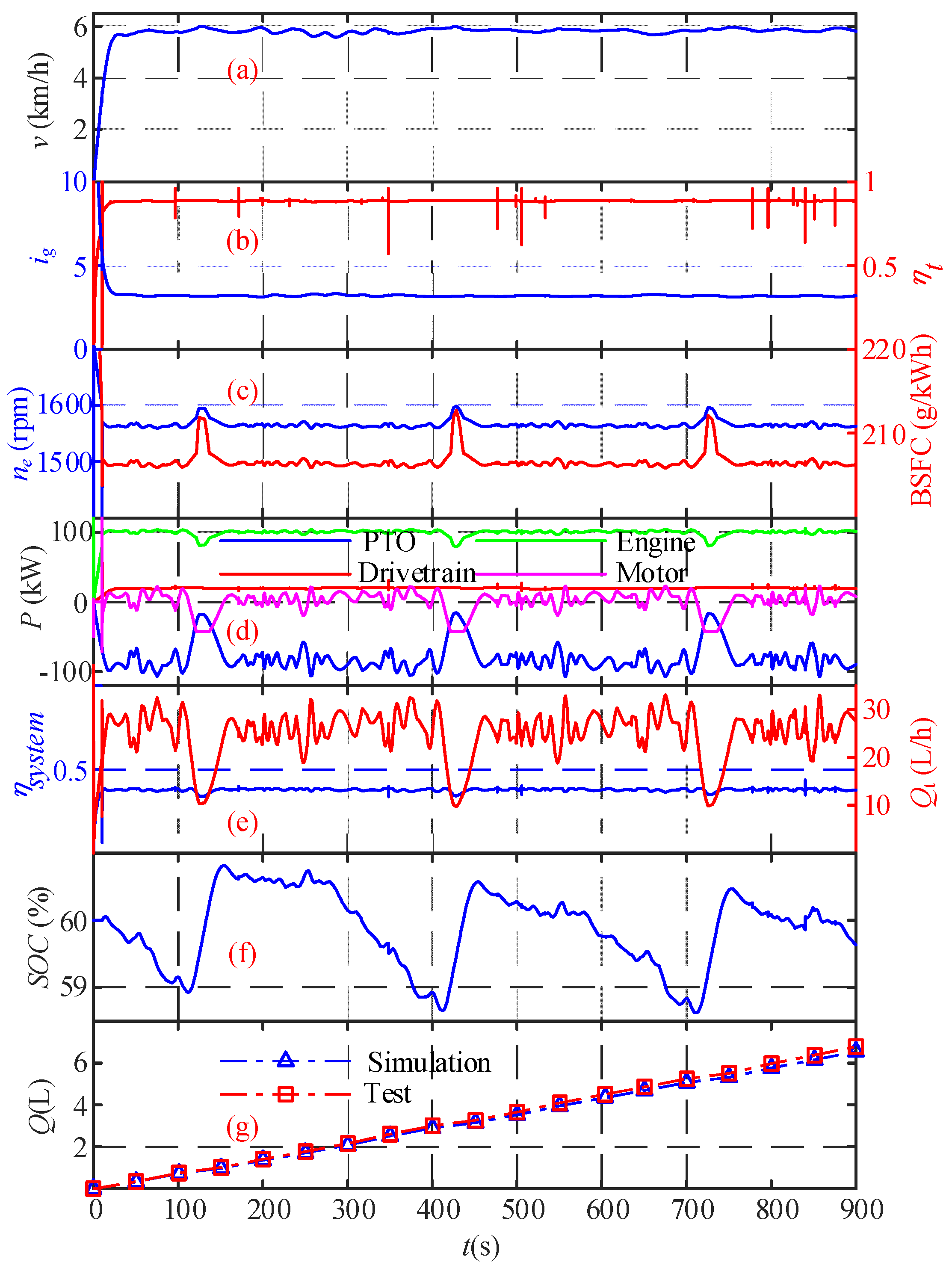
5.3.2. Harvest Analysis
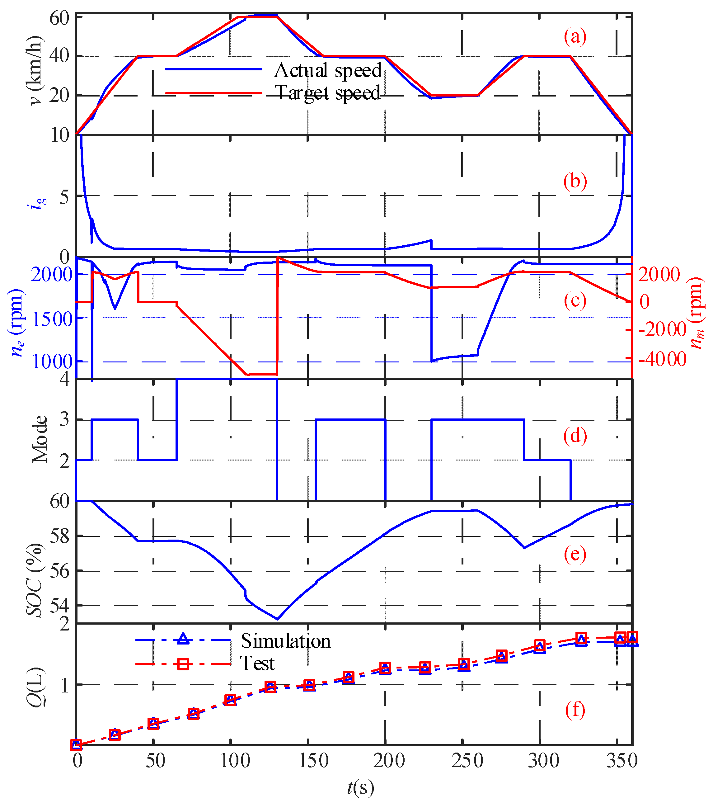
5.3.3. Transport Analysis
6. Discussion
- In terms of structural design, compared to a typical hydro-mechanical transmission, this paper uses only a single planetary row for the merging of the hydraulic and mechanical power, which has fewer planetary gears compared to the structure mentioned in the paper [41]. Moreover, the advantages of hybrid power can be exploited without the need for more powerful electrical equipment.
- The speed ratio control strategy and energy management strategy are designed for the hybrid tractor, and three tractor operating conditions of the whole tractor is simulated. Moreda pointed out that there are no standard test conditions for hybrid tractors, however, the data from the actual tractor operation is reliable and can be a reference for the research of hybrid tractors [42].
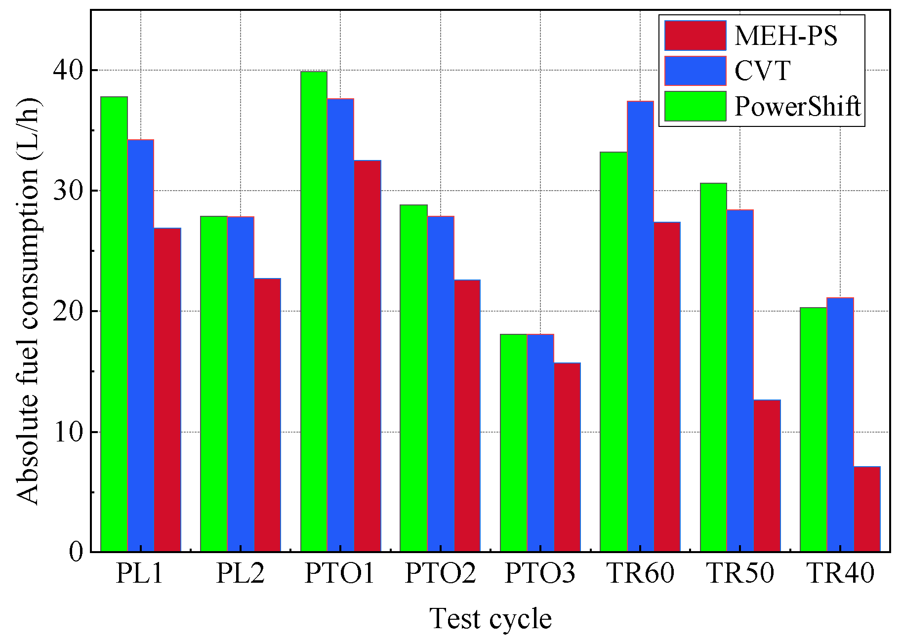
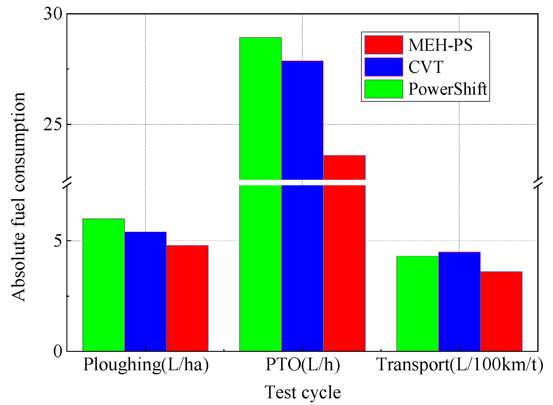
- The feasibility of the MEH-PS scheme was confirmed by comparing the difference between bench test and simulation data within 5% and comparing the fuel consumption of PowerShift tractors and CVT tractors published by DLG under the corresponding operating conditions. It was found that the device has the lowest fuel consumption, which further confirms the reliability of the scheme, and the scheme has practical value for energy saving of agricultural machinery.
7. Conclusions
8. Patents
Author Contributions
Funding
Institutional Review Board Statement
Informed Consent Statement
Data Availability Statement
Conflicts of Interest
Appendix A

| Item | Parameter | Specification |
|---|---|---|
| Tractor | Mass | 8260 kg |
| Radius of wheels | 750 mm | |
| Engine | Rated power | 132 kW@2200 r/min |
| Maximum torque | 750 Nm@1300 r/min | |
| Minimum fuel consumption | 203 g/kW·h@1500 r/min | |
| Motor | Rated power | 45 kW |
| Rated speed | 3300 r/min | |
| Maximum speed | 11,000 r/min | |
| Battery | Capacity | 45 Ah |
| Nominal voltage | 360 V | |
| Driveline | Transmission ratio | 0.63~4.33 |
| Gear ratio of main reducer | 6.4 | |
| Gear ratio of wheel reducer | 3.7 |
| Load Type | Test Cycle | Engine Speed (r/min) | Driving Speed (km/h) | Absolute Fuel Consumption (L/h) | BSFC (g/kWh) | ||||||||
|---|---|---|---|---|---|---|---|---|---|---|---|---|---|
| PowerShift | CVT | MEH-PS | PowerShift | CVT | MEH-PS | PowerShift | CVT | MEH-PS | PowerShift | CVT | MEH-PS | ||
| Drawbar work | PL1 | 1407 | 1348 | 1684 | 7.1 | 6.7 | 7.0 | 37.8 | 34.2 | 26.9 | 247 | 251 | 208 |
| PL2 | 1312 | 1393 | 1407 | 8.5 | 8.8 | 9.1 | 27.9 | 27.8 | 22.7 | 246 | 250 | 205 | |
| Drawbar + PTO work | PTO1 | 1663 | 1622 | 1558 | 5.6 | 5.7 | 5.7 | 39.9 | 37.6 | 32.5 | 227 | 230 | 206 |
| PTO2 | 1424 | 1664 | 1567 | 5.5 | 5.9 | 5.8 | 28.8 | 27.9 | 22.6 | 227 | 236 | 207 | |
| PTO3 | 1433 | 1684 | 1574 | 5.5 | 5.9 | 5.8 | 18.1 | 18.1 | 15.7 | 249 | 266 | 207 | |
| Transport work | TR60 | 1989 | 1448 | 2140 | 60.3 | 61.2 | 60.1 | 33.2 | 37.4 | 27.4 | 573 | 580 | 259 |
| TR50 | 1908 | 1201 | 2135 | 51.1 | 50.4 | 50.0 | 30.0 | 28.4 | 12.6 | 539 | 610 | 266 | |
| TR40 | 1478 | 1015 | 2079 | 40.8 | 40.2 | 40.0 | 20.3 | 21.0 | 7.09 | 266 | 643 | 236 | |
References
- Data Query System of Ministry of Agriculture and Rural Affairs of the People’s Republic of China. Available online: http://zdscxx.moa.gov.cn:8080/nyb/pc/search.jsp (accessed on 26 February 2022).
- The State Council on the Issuance of the “13th Five-Year Plan” Comprehensive Work Program of Energy Saving and Emission Reduction Notice. Available online: http://www.gov.cn/zhengce/content/2017-01/05/content_5156789.htm# (accessed on 5 January 2017).
- Opinions on the Key Work of Comprehensive Promotion of Rural Revitalization in 2022. Available online: https://xhpfmapi.xinhuaxmt.com/vh512/share/10614093 (accessed on 22 February 2022).
- Scolaro, E.; Alberti, L.; Barater, D. Electric Drives for Hybrid Electric Agricultural Tractors. In Proceedings of the 2021 IEEE Workshop on Electrical Machines Design, Control and Diagnosis (WEMDCD), Modena, Italy, 8–9 April 2021; pp. 331–336. [Google Scholar]
- Renius, K.T.; Resch, R. Continuously Variable Tractor Transmissions; American Society of Agricultrual Engineers: St. Joseph, MI, USA, 2005. [Google Scholar]
- Yu, J.; Cao, Z.; Cheng, M.; Pan, R. Hydro-mechanical power split transmissions: Progress evolution and future trends. Proc. Inst. Mech. Eng. Part D J. Automob. Eng. 2019, 233, 727–739. [Google Scholar] [CrossRef]
- Xia, Y.; Sun, D.; Qin, D.; Zhou, X. Optimisation of the power-cycle hydro-mechanical parameters in a continuously variable transmission designed for agricultural tractors. Biosyst. Eng. 2020, 193, 12–24. [Google Scholar] [CrossRef]
- Li, B.; Sun, D.; Hu, M.; Zhou, X.; Wang, D.; Xia, Y.; You, Y. Automatic gear-shifting strategy for fuel saving by tractors based on real-time identification of draught force characteristics. Biosyst. Eng. 2020, 193, 46–61. [Google Scholar] [CrossRef]
- Wan, L.; Dai, H.; Zeng, Q.; Sun, Z.; Tian, M. Characteristic analysis and co-validation of hydro-mechanical continuously variable transmission based on the wheel loader. Appl. Sci. 2020, 10, 5900. [Google Scholar] [CrossRef]
- Rossetti, A.; Macor, A. Control strategies for a powertrain with hydromechanical transmission. Energy Procedia 2018, 148, 978–985. [Google Scholar] [CrossRef]
- Xiao, M.; Zhao, J.; Wang, Y.; Zhang, H.; Lu, Z.; Wei, W. Fuel economy of multiple conditions self-adaptive tractors with hydro-mechanical CVT. Int. J. Agric. Biol. Eng. 2018, 11, 102–109. [Google Scholar] [CrossRef]
- Ahn, S.; Choi, J.; Kim, S.; Lee, J.; Choi, C.; Kim, H. Development of an integrated engine-hydro-mechanical transmission control algorithm for a tractor. Adv. Mech. Eng. 2015, 7, 1–18. [Google Scholar] [CrossRef]
- Karner, J.; Baldinger, M.; Reichl, B. Prospects of hybrid systems on agricultural machinery. GSTF J. Agric. Eng. 2014, 1, 33–37. [Google Scholar] [CrossRef]
- Delgado, O.; Lutsey, N. Advanced Tractor-Trailer Efficiency Technology Potential in the 2020–2030 Timeframe; The International Council on Clean Transportation: Washington, DC, USA, 2015; Report in preparation. [Google Scholar]
- Mcfadzean, B.; Butters, L. An investigation into the feasibility of hybrid and all-electric agricultural machines. Sci. Pap. Ser. A Agron 2017, 60, 500–511. [Google Scholar]
- Katrašnik, T. Energy conversion phenomena in plug-in hybrid-electric vehicles. Energy Convers. Manag. 2011, 52, 2637–2650. [Google Scholar] [CrossRef]
- Guo, H.; Wang, X.; Li, L. State-of-charge-constraint-based energy management strategy of plug-in hybrid electric vehicle with bus route. Energy Convers. Manag. 2019, 199, 111972. [Google Scholar] [CrossRef]
- Lee, D.; Kim, Y.; Choi, C.; Chung, S.; Inoue, E.; Okayasu, T. Development of a parallel hybrid system for agricultural tractors. J. Fac. Agric. Kyushu Univ. 2017, 62, 137–144. [Google Scholar] [CrossRef]
- Kim, W.-S.; Kim, Y.-J.; Chung, S.-O.; Lee, D.-H.; Choi, C.-H.; Yoon, Y.-W. Development of simulation model for fuel efficiency of agricultural tractor. Korean J. Agric. Sci. 2016, 43, 116–126. [Google Scholar] [CrossRef] [Green Version]
- Li, X.; Zhang, L.; Yang, S.; Liu, N. Analysis and experiment of HMT stationary shift control considering the effect of oil bulk modulus. Adv. Mech. Eng. 2020, 12, 1–13. [Google Scholar] [CrossRef]
- Rossi, C.; Pontara, D.; Falcomer, C.; Bertoldi, M.; Mandrioli, R. A Hybrid–Electric Driveline for Agricultural Tractors Based on an e-CVT Power-Split Transmission. Energies 2021, 14, 6912. [Google Scholar] [CrossRef]
- Zhu, Z.; Lai, L.; Sun, X.; Chen, L.; Cai, Y. Design and Analysis of a Novel Mechanic-Electronic-Hydraulic Powertrain System for Agriculture Tractors. IEEE Access 2021, 9, 153811–153823. [Google Scholar] [CrossRef]
- Haughery, J.R.; Steward, B.L.; Ryan, S.J.; Kankanamalage, R.G. Modeling Hybrid Hydro-Electro-Mechanical Power-Split Propulsion Systems. In Proceedings of the Fluid Power Systems Technology, Virtual, 19–21 October 2021; p. V001T001A047. [Google Scholar]
- Cheng, Z.; Lu, Z.; Qian, J. A new non-geometric transmission parameter optimization design method for HMCVT based on improved GA and maximum transmission efficiency. Comput. Electron. Agric. 2019, 167, 105034. [Google Scholar] [CrossRef]
- Hui, S.; Lifu, Y.; Junqing, J.; Yanling, L. Control strategy of hydraulic/electric synergy system in heavy hybrid vehicles. Energy Convers. Manag. 2011, 52, 668–674. [Google Scholar] [CrossRef]
- Onori, S.; Serrao, L.; Rizzoni, G. Hybrid Electric Vehicles: Energy Management Strategies; Springer: London, UK, 2016. [Google Scholar]
- Liu, T.; Tang, X.; Wang, H.; Yu, H.; Hu, X. Adaptive hierarchical energy management design for a plug-in hybrid electric vehicle. IEEE Trans. Veh. Technol. 2019, 68, 11513–11522. [Google Scholar] [CrossRef]
- Ince, E.; Güler, M.A. Design and analysis of a novel power-split infinitely variable power transmission system. J. Mech. Des. 2019, 141, 054501. [Google Scholar] [CrossRef]
- Manring, N.D. Mapping the efficiency for a hydrostatic transmission. J. Dyn. Syst. Meas. Control. 2016, 138, 031004. [Google Scholar] [CrossRef]
- Renius, K.T. Fundamentals of Tractor Design; Springer: Cham, Switzerland, 2020. [Google Scholar]
- Carl, B.; Ivantysynova, M.; Williams, K. Comparison of Operational Characteristics in Power Split Continuously Variable Transmissions; Sae technical paper; SAE: Warrendale, PA, USA, 2006; ISSN 0148-7191. [Google Scholar]
- Chancellor, W.; Thai, N. Automatic control of tractor transmission ratio and engine speed. Trans. ASAE 1984, 27, 642–0646. [Google Scholar] [CrossRef]
- Hofman, T.; Steinbuch, M.; Van Druten, R.; Serrarens, A. Rule-based energy management strategies for hybrid vehicles. Int. J. Electr. Hybrid Veh. 2007, 1, 71–94. [Google Scholar] [CrossRef]
- Gu, B.; Rizzoni, G. An adaptive algorithm for hybrid electric vehicle energy management based on driving pattern recognition. In Proceedings of the ASME International Mechanical Engineering Congress and Exposition, Chicago, IL, USA, 5–10 November 2006; pp. 249–258. [Google Scholar]
- Zhang, L.; Liu, W.; Qi, B. Energy optimization of multi-mode coupling drive plug-in hybrid electric vehicles based on speed prediction. Energy 2020, 206, 118126. [Google Scholar] [CrossRef]
- Wang, F.; Xia, J.; Xu, X.; Cai, Y.; Ni, S.; Que, H. Torsional vibration-considered energy management strategy for power-split hybrid electric vehicles. J. Clean. Prod. 2021, 296, 126399. [Google Scholar] [CrossRef]
- Zhang, L.; Liu, W.; Qi, B. Innovation design and optimization management of a new drive system for plug-in hybrid electric vehicles. Energy 2019, 186, 115823. [Google Scholar] [CrossRef]
- Gökce, K.; Ozdemir, A. An instantaneous optimization strategy based on efficiency maps for internal combustion engine/battery hybrid vehicles. Energy Convers. Manag. 2014, 81, 255–269. [Google Scholar] [CrossRef]
- Xia, Y.; Sun, D.; Qin, D.; Hou, W. Study on the Design Method of a New Hydro-Mechanical Continuously Variable Transmission System. IEEE Access 2020, 8, 195411–195424. [Google Scholar] [CrossRef]
- Han, J.; Xia, C.; Shang, G.; Gao, X. In-field experiment of electro-hydraulic tillage depth draft-position mixed control on tractor. In Proceedings of the IOP Conference Series: Materials Science and Engineering, Changsha, China, 28–29 October 2017; p. 012028. [Google Scholar]
- Liu, F.; Wu, W.; Hu, J.; Yuan, S. Design of multi-range hydro-mechanical transmission using modular method. Mech. Syst. Signal Processing 2019, 126, 1–20. [Google Scholar] [CrossRef]
- Moreda, G.; Muñoz-García, M.; Barreiro, P. High voltage electrification of tractor and agricultural machinery—A review. Energy Convers. Manag. 2016, 115, 117–131. [Google Scholar] [CrossRef]


| Driving Mode | C1 | C2 | C3 | B1 |
|---|---|---|---|---|
| Pure electric drive (1) | ▲ | ▲ | ||
| Pure engine drive (2) | ▲ | ▲ | ||
| Torque coupling drive (3) | ▲ | ▲ | ▲ | |
| Speed coupling drive (4) | ▲ | ▲ |
| Gear | C4 | C5 | B1 | B2 | B3 | B4 | B5 | ig |
|---|---|---|---|---|---|---|---|---|
| F(H) | ▲ | ▲ | ▲ | |||||
| R(H1) | ▲ | ▲ | ▲ | |||||
| R(H2) | ▲ | ▲ | ▲ | |||||
| F (HM1) | ▲ | ▲ | ▲ | |||||
| F (HM2) | ▲ | ▲ | ▲ | |||||
| R(HM) | ▲ | ▲ | ▲ | |||||
| F (M1) | ▲ | ▲ | ▲ | |||||
| F (M2) | ▲ | ▲ | ▲ | |||||
| R(M) | ▲ | ▲ | ▲ |
| Parameters | k1 | k2 | k3 | k4 | i1 | i2 |
|---|---|---|---|---|---|---|
| Value | 1.80 | 1.60 | 1.65 | 1.65 | 0.62 | 1.00 |
| Time (s) | Tractor Speed (km/h) | Ploughing Depth (m) |
|---|---|---|
| 0~100 | 9.00 | 0.10 |
| 100~200 | 9.00 | 0.18 |
| 200~300 | 9.00 | 0.26 |
| 300~400 | 7.00 | 0.34 |
| Parameter | Ploughing | Harvest | Transport |
|---|---|---|---|
| SOC initial value/final value (%) | 60.00/61.96 | 60.00/59.63 | 60.00/59.81 |
| SOC difference (%) | +1.96 | −0.37 | −0.19 |
| Simulation/test fuel consumption (L) | 2.59/2.72 | 6.56/6.80 | 1.69/1.77 |
| Fuel consumption error (%) | 4.8 | 3.5 | 4.5 |
Publisher’s Note: MDPI stays neutral with regard to jurisdictional claims in published maps and institutional affiliations. |
© 2022 by the authors. Licensee MDPI, Basel, Switzerland. This article is an open access article distributed under the terms and conditions of the Creative Commons Attribution (CC BY) license (https://creativecommons.org/licenses/by/4.0/).
Share and Cite
Zhu, Z.; Yang, Y.; Wang, D.; Cai, Y.; Lai, L. Energy Saving Performance of Agricultural Tractor Equipped with Mechanic-Electronic-Hydraulic Powertrain System. Agriculture 2022, 12, 436. https://doi.org/10.3390/agriculture12030436
Zhu Z, Yang Y, Wang D, Cai Y, Lai L. Energy Saving Performance of Agricultural Tractor Equipped with Mechanic-Electronic-Hydraulic Powertrain System. Agriculture. 2022; 12(3):436. https://doi.org/10.3390/agriculture12030436
Chicago/Turabian StyleZhu, Zhen, Yanpeng Yang, Dongqing Wang, Yingfeng Cai, and Longhui Lai. 2022. "Energy Saving Performance of Agricultural Tractor Equipped with Mechanic-Electronic-Hydraulic Powertrain System" Agriculture 12, no. 3: 436. https://doi.org/10.3390/agriculture12030436