Article

Dynamic Fresh Weight Prediction of Substrate-Cultivated Lettuce Grown in a Solar Greenhouse Based on Phenotypic and Environmental Data

1
College of Mechanical & Electronic Engineering, Shandong Agricultural University, Tai’an 271018, China
2
Shandong Provincial Key Laboratory of Horticultural Machinery and Equipment, Tai’an 271018, China
3
Shandong Agricultural Equipment Intelligent Engineering Laboratory, Tai’an 271018, China
4
School of Mechanical Engineering, Shanghai Jiao Tong University, Shanghai 200240, China
*
Authors to whom correspondence should be addressed.
Agriculture 2022, 12(11), 1959; https://doi.org/10.3390/agriculture12111959
Submission received: 12 October 2022 / Revised: 13 November 2022 / Accepted: 17 November 2022 / Published: 20 November 2022
(This article belongs to the Special Issue Robots and Autonomous Machines for Agriculture Production)

Abstract

:
The fresh weight of vegetables is an important index for the accurate evaluation of growth processes, which are affected by factors such as temperature and radiation fluctuation, especially in a passive solar greenhouse. Predicting dynamic growth indexed by fresh weight in a solar greenhouse remains a challenge. A novel method for predicting the dynamic growth of leafy vegetables based on the in situ sensing of phenotypic and environmental data of batches is proposed herein, enabling prediction of the dynamic fresh weight of substrate-cultivated lettuce grown in a solar greenhouse under normal water and fertilizer conditions. Firstly, multibatch lettuce cultivation experiments were carried out and batch datasets constructed by collecting growth environmental data and lettuce canopy images in real time. Secondly, the cumulative environmental factors and instantaneous fresh weights of the lettuce batches were calculated. The optimum response time in days was then explored through the most significant correlations between cumulative environmental factors and fresh weight growth. Finally, a dynamic fresh weight prediction model was established using a naive Bayesian network, based on cumulative environmental factors, instantaneous fresh weight, and the fresh weight increments of batches. The results showed that the computing time setpoint of cumulative environmental factors and instantaneous fresh weight of lettuce was 8:00 AM and the optimum response time was 12 days, and the average R2 values among samples from three batches reached 95.95%. The mean relative error (MRE) of fresh weight prediction 4 days into the future based on data from the current batch was not more than 9.57%. Upon introducing another batch of data, the prediction 7 days into the future dropped below 8.53% MRE; upon introducing another two batches, the prediction 9 days into the future dropped below 9.68% MRE. The accuracy was improved by the introduction of additional data batches, proving the model’s feasibility. The proposed dynamic fresh weight growth prediction model can support the automatic management of substrate-cultivated leafy vegetables in a solar greenhouse.

1. Introduction

In line with an annual increase in greenhouse planting area in recent years [1,2], the solar greenhouse, a relatively low-cost, environmentally controllable, and highly productive option for farmers, has become the predominant facility type used to provide year-round vegetable production in northern China [3,4]. A solar greenhouse has a large roof area along the south side which is passively heated by sunlight during the daytime [5]. Meanwhile, a thermal blanket is rolled over the greenhouse at night to hold heat inside the structure, and a northern brick wall preserves heat inside the structure [6]. Compared with Venlo greenhouses [7], passive solar greenhouses generally provide only basic environmental control with low-cost equipment [8]. In addition, the use of advanced automated fertigators to ensure sufficient water and fertilizer absorption of vegetables in solar greenhouses has become popular owing to significant labor savings [9]. In production in a Venlo greenhouse, environmental control technology [10,11] is used to regulate indoor environmental parameters such as light, temperature, humidity, and carbon dioxide, making the vegetable growth environment close to optimal. Solar greenhouses have the disadvantages of large temperature fluctuation ranges and frequently weak solar radiation [12], which is not conducive to crop growth, making the crop growth models established in Venlo greenhouse systems unsuitable for application in solar greenhouses.
In a suitable environment, vegetable growth adheres to certain inherent laws throughout the plant’s life cycle [13]. Scholars have studied many crop growth models [14,15,16,17] with the aim of guiding future crop production in greenhouse systems through regulation of the environment, water, and fertilizer. In one greenhouse crop growth system, a machine learning method based on the expectation maximum algorithm was applied to link environmental parameters with crop growth [18]. Based on only a small number of samples, future crop growth could be predicted several days in advance. Thus, the feasibility of using environmental parameters to predict vegetable growth in greenhouse systems has been verified. However, in the above-mentioned model, leaf area index, evapotranspiration, and dry weight were taken as crop growth indicators, and the leaf area index and dry weight were obtained by destructive methods at intervals of one week. For one thing, indicators obtained using destructive methods cannot provide growth indicators over the whole life cycle sequence of a specific plant, and indicators for shorter time intervals were not obtained. For another, many vegetables needed to be planted in order to assess indicators using destructive sampling during the vegetable growth period, and the process was inefficient and cumbersome. Moreover, the indicators used to measure vegetable growth could not directly reflect the current vegetable yield (i.e., fresh weight).
The fresh weight of vegetables is an important index for accurate evaluation of the growth process, so it is of great significance to apply the fresh weight index to the prediction of crop growth. Compared with hydroponic vegetables, the online, nondestructive monitoring of the fresh weight of substrate-cultured vegetables during the growth process is a challenge. In view of the importance of fresh weight, Yanes et al. [19] proposed a deep learning image segmentation method to obtain information from canopy images for the estimation of fresh weight of hydroponic lettuce, and a regression model relating lettuce size and fresh weight was established. Jung et al. [20] established a model of the relationship between the projected area of lettuce canopy and fresh weight in an environmentally controllable, water-based lettuce cultivation system based on the morphological analysis machine vision method. Jiang et al. [21] developed a fresh weight estimation system for hydroponic lettuce based on online image processing, which realized high-precision estimation of the fresh weight of lettuce and allowed environmental control for high-quality production. In hydroponic vegetable production systems, the plants can be removed from the nutrient solution temporarily and directly weighed without hindering their continuous growth. This is convenient for nondestructive calibration of fresh weight and makes it easy to realize nondestructive, high-precision fresh weight estimation. In substrate culture systems, the plants can be taken out of the substrate and directly weighed to accurately obtain the fresh weight. However, plants weighed in this way will not continue to grow [22,23], and the subsequent fresh weight growth cannot be obtained. It is difficult to achieve nondestructive estimation of the fresh weight of substrate-cultivated vegetables. In order to solve this problem, Liu et al. [24] proposed a fresh weight estimation method based on the fusion of phenotypic characteristics and environmental parameters, which was used to realize nondestructive estimation of the individual and population fresh weights of substrate-cultured lettuce in a solar greenhouse.
However, accurate prediction of dynamic fresh weight growth based on in situ sensing in solar greenhouse systems is still a challenge. Fresh weight growth of vegetables is affected by many complex environmental factors [25]. Large indoor temperature fluctuations and frequently weak solar radiation in solar greenhouse systems lead to differences in the fresh weight growth of different batches. There is a complex and uncertain relationship between vegetable fresh weight growth and environmental factors. Therefore, in contrast to the static modeling of fresh weight under hydroponic conditions [19], a novel prediction method for the dynamic growth of leafy vegetables based on phenotypic and environmental data of batches is proposed herein, which is able to predict the dynamic fresh weight of substrate-cultivated lettuce in a solar greenhouse system under normal water and fertilizer conditions.
The main contributions of this paper are as follows:
(1) Multibatch substrate-cultivated lettuce cultivation experiments were carried out, with the growth environment and lettuce canopy images monitored in real time. A dataset was built using phenotypic and environmental data of batches.
(2) Computation of the cumulative environmental factors and instantaneous fresh weight of batches of lettuce was achieved. The optimum response time was explored via the most significant correlations between cumulative environmental factors and fresh weight growth.
(3) A dynamic fresh weight prediction model was established using a naive Bayesian network, based on cumulative environmental factors, instantaneous fresh weight, and fresh weight increments of batches, which can be used to predict the dynamic fresh weight of substrate-cultured lettuce in a solar greenhouse system.

2. Materials and Methods

2.1. Experimental Design

The experimental site was Solar Greenhouse No. 6 in Shandong Agricultural University Science and Technology Innovation Park, located in Tai’an City, Shandong Province, China (36.16° N, 117.16° E). The greenhouse has a span of about 8 m, a height of about 4 m, and a length of about 50 m from east to west. The experimental material was Italian lettuce, which was produced by Hebei Maohua Seed Industry Limited Company. The main characteristics of this lettuce are a semi-erect form, plant height of about 26 cm, development of about 28 cm, and nearly round leaves. The color is emerald green, and the loose leaves do not form a ball. In order to improve the accuracy of the dynamic fresh weight prediction model, multiple batches of planting experiments were carried out. The same variety of lettuce was used for the multiple batches of planting experiments. When the lettuce seedlings in a batch had grown to five leaves and a heart, the batch was transplanted into a planting tank filled with substrate.
The aboveground growth environment of the lettuce was the closed microclimate environment of the passive solar greenhouse. Due to the structural characteristics of a passive solar greenhouse, only simple environmental regulation could be achieved during the lettuce growth process, barring the introduction of heating, fans, supplementary lights, etc. For example, in the morning, the thermal blanket was opened to allow storage of heat from the sunlight. At noon, the vent was opened to allow natural ventilation for dehumidification, cooling, and air exchange. In the evening, the thermal blanket was closed for insulation, so as to ensure a normal indoor lettuce growth environment and prevent frostbite of the lettuce plants. The underground growth environment of the lettuce plants was the substrate. The substrate had the characteristics of good ventilation and a good drainage effect, but the water retention effect was relatively poor. Therefore, Yamazaki formula nutrient solution at a 100% concentration was used for irrigation via the water and fertilizer application system in the greenhouse (Figure 1), ensuring normal water and fertilizer conditions throughout the lettuce cultivation experiment.

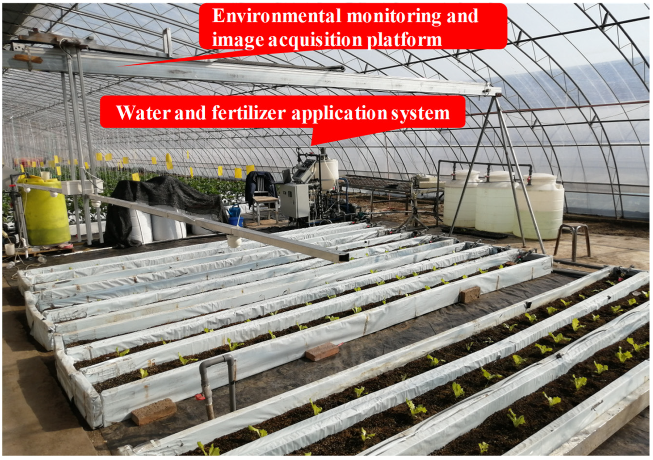
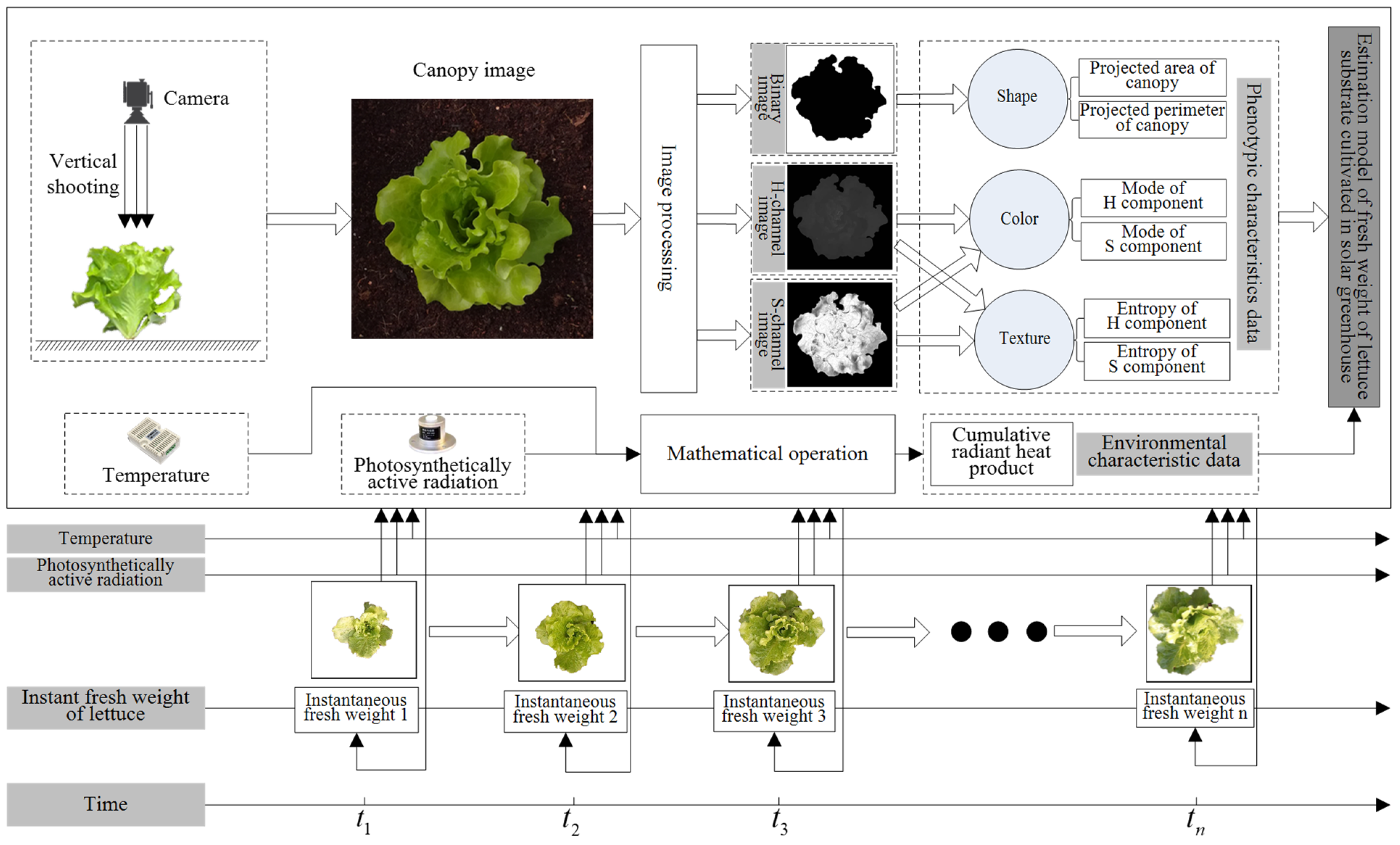
2.2. Acquisition of Environmental Data and Lettuce Images in the Solar Greenhouse

An environmental monitoring and image acquisition platform (Figure 1) was used to record the temperature, humidity, photosynthetically active radiation, carbon dioxide concentration, and lettuce canopy images in the solar greenhouse during the lettuce cultivation experiment. The platform was mainly composed of a support mechanism, guide rail slide, hanger, cross bar, sensor, and controller. The support mechanism was used to support the guide rail slide so that the guide rail slide could move horizontally in the north–south direction at a certain height from the ground. The guide rail slide was fixed at the upper end of the support mechanism and the cross bar equipped with the sensor was connected through the hanger, so that the sensor could move in the north–south direction synchronously with the cross bar. The height of the cross bar could be adjusted according to the current situation, and the cross bar and the guide rail slide were kept vertical in the horizontal direction. The guide rail slide was controlled by the controller and the cross bar equipped with sensors was moved to complete the environmental monitoring and image acquisition tasks in the upper part of the planting area.

2.3. Calculation of Environmental Factors and Instantaneous Fresh Weight

2.3.1. Calculation of Cumulative Radiant Heat Product

The effects of temperature and radiation on the fresh weight of lettuce can be measured by the cumulative radiant heat product. The specific calculation formula is as follows [26]:
R T E = { 0                           ( T < T b ) T T b T o b T b               ( T b T < T o b )       1                     ( T o b T T o u ) T m T T m T o u             ( T o u < T T m ) 0                         ( T > T m )  
T E P = R T E P    
R T E P = i = 1 24 ( R T E i × P A R i × 3600 / 10 6 )
where Tb is the lower limit of growth temperature (°C), Tm is the upper limit of growth temperature (°C), Tob is the lower limit of optimum growth temperature (°C), Tou is the upper limit of optimum growth temperature (°C), T is the ambient temperature (°C), RTE is the relative thermal effect, RTEP is the daily cumulative radiant heat product (MJ·m−2·d−1), RTEi is the relative thermal effect in the i-th hour, PAri is the average photosynthetically active radiation in the i-th hour (MJ·m−2·d−1), and TEP is the cumulative radiation heat product (MJ·m−2).

2.3.2. Calculation of Crop Evapotranspiration

If reference evapotranspiration is used to replace crop evapotranspiration, there will be a large error. Therefore, in order to improve the accuracy of calculation of crop evapotranspiration, the crop coefficient was used to correct the reference evapotranspiration. The specific calculation formula is as follows [27]:
E T c = E T 0 K c
E T 0 i = 0.408 Δ ( R n G ) + γ 1713 T + 273 ( e s e a ) Δ + 1.64 γ  
Δ = 2505 exp ( 17.27 T T + 237.3 ) ( T + 237.3 ) 2
e s = e s ( T max ) + e s ( T min ) 2
e s ( T max / min ) = 0.6108 exp ( 17.27 T max / min T max / min + 237.3 )
e a = e s ( T min ) R H max 100 + e s ( T max ) R H min 100 2
R = K P A R
R n = a · R + b
where ET0 is the reference evapotranspiration under full irrigation (cm·d−1), Δ is the slope of the saturated vapor pressure curve (kPa·°C−1), Rn is the net radiation of the crop canopy (MJ·m−2·d−1), G is the soil heat flux density (MJ·m−2·d−1), γ is the dry and wet table constant (kPa·°C−1), T is the daily average temperature at the height of 1.5 to 2.5 m above the surface (°C), Tmax/min is the daily maximum or minimum air temperature at the height of 1.5 to 2.5 m above the surface (°C), es is the average saturated vapor pressure at the height of 1.5 to 2.5 m above the surface (kPa), ea is the average actual vapor pressure at the height of 1.5 to 2.5 m above the surface (kPa), RHmax/min is the daily maximum or minimum relative humidity at the height of 1.5 to 2.5 m above the surface (%), ETci is the evapotranspiration of crops on the i-th day under full irrigation (cm/d), Kc is the crop coefficient, R is the total solar radiation (MJ·m−2·d−1), PAR is the photosynthetically active radiation (MJ·m−2·d−1), K is the conversion coefficient between photosynthetically active radiation and total solar radiation, and a and b are the conversion coefficients between net radiation and total radiation.
If G = 0, γ = 0.067, Kc = 0.7, 1.00 or 0.95 [28], K = 80/39 [29], a = 0.8277, and b = 0.2909 [30], then ETc can be calculated using Formulas (4)–(11) and the indoor temperature, humidity, and photosynthetically active radiation.

2.3.3. Calculation of Instantaneous Fresh Weight and Fresh Weight Increment

Based on the previous research results of this research group [24], the online, nondestructive calculation of the fresh weight of substrate-cultivated lettuce grown in a solar greenhouse was realized by combining the data of phenotypic characteristics and environmental characteristics. Firstly, the collected lettuce canopy images were used to extract phenotypic characteristics such as shape, color, and texture. Then, using the online monitoring values of temperature and photosynthetically active radiation, cumulative radiant heat product was calculated as an environmental factor. Finally, the above factors were introduced into the model for fresh weight estimation of substrate-cultivated lettuce grown in a solar greenhouse, and the instantaneous fresh weight of the lettuce was obtained (Figure 2). The fresh weight increment was obtained by subtracting the instantaneous fresh weight at one time point from another.

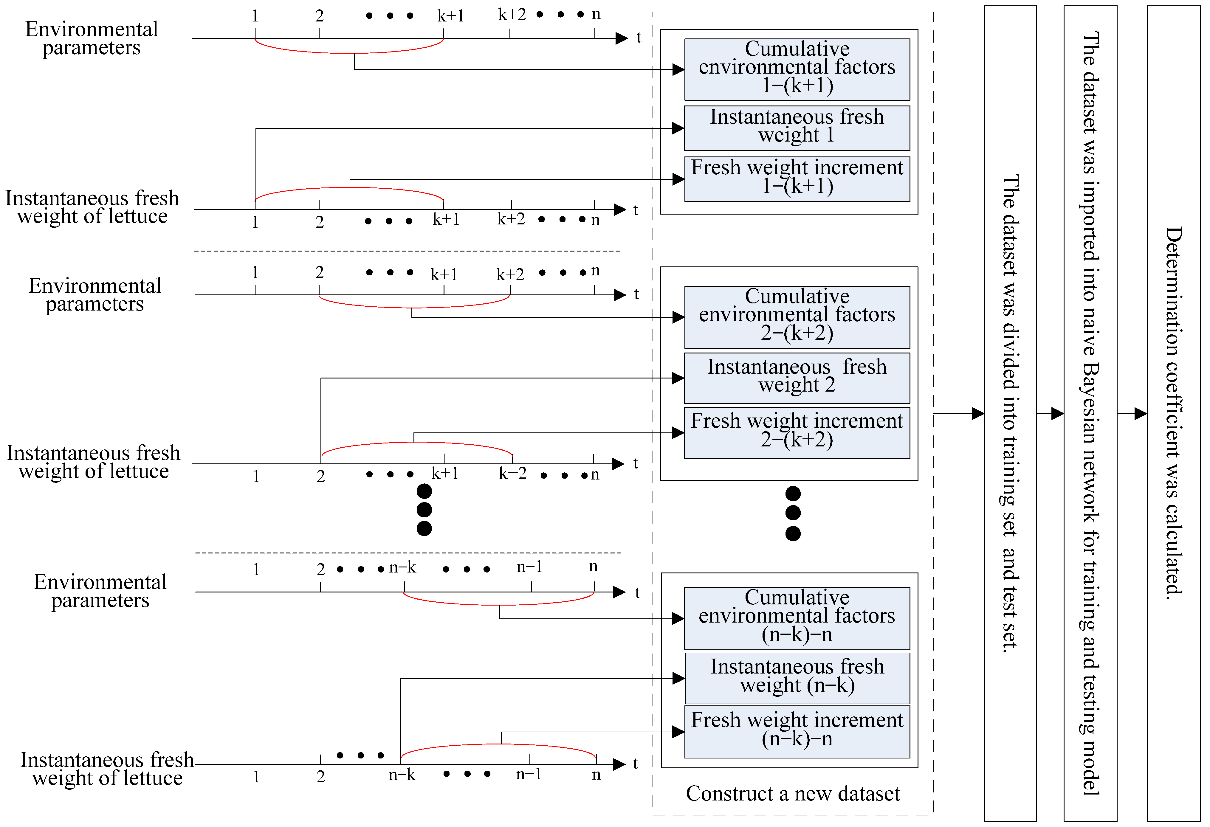
2.4. Exploration of Optimum Response Time in Days

In order to study the optimum response time of the most significant correlations between cumulative environmental factors and fresh weight growth, a naive Bayesian network [31,32,33] was used to establish the relationship model. There were n − k elements in the dataset, including cumulative environmental factors, instantaneous fresh weight, and fresh weight increments of the previous k days, and the dataset was divided into a training set and a test set. The training set was introduced into the naive Bayesian network for model training, and the test set was used for model testing.
The determination coefficient of the model was calculated by referring to Formula (12) using predicted values and measured values, and was used to examine the degree of correlation between predicted values and measured values of the samples in the dataset. The normal value range is from 0 to 1, and the closer it is to 1, the better the model fits the data. The calculation formula is as follows:
R 2 = 1 i = 1 n ( y _ t e s t i y _ p r e i ) 2 i = 1 n ( y _ t e s t i y _ m e a n ) 2
where y_testi is the measured value of the i-th sample in the dataset (g), y_prei is the predicted value of the i-th sample in the dataset (g), and y_mean is the average of the measured values of all samples in the dataset (g).
The coefficient of determination was used as the evaluation index of the model. The larger the coefficient of determination, the more significant the relationship between cumulative environmental factors and fresh weight growth.
The solution process with the most significant response between cumulative environmental factors and fresh weight growth in the previous k days is shown in Figure 3. The figures on the y axis represent the environmental parameters (temperature, humidity, photosynthetically active radiation, and carbon dioxide concentration) or the instantaneous fresh weight of lettuce at a certain time. Firstly, instantaneous fresh weight on day 1, cumulative environmental factors (cumulative radiant heat product, crop evapotranspiration, and average carbon dioxide concentration), and fresh weight increment from day 1 to day k + 1 were taken as the first element group in constructing the dataset. The instantaneous fresh weight on day 2, cumulative environmental factors, and fresh weight increment from day 2 to day k + 2 were used as the second element group in constructing the dataset. Correspondingly, instantaneous fresh weight on day n – k, cumulative environmental factors, and fresh weight increment from day n − k to day n were taken as the last element group in constructing the dataset, which had a total of n – k element groups. The dataset was then divided into a training set and a test set, and the training set was substituted into the naive Bayesian network for model training. Finally, the test set was substituted into the above model and the determination coefficient was calculated, which was used as the evaluation index for the significance of the response between cumulative environmental factors and fresh weight growth in the previous k days.

2.5. Establishment of Dynamic Fresh Weight Growth Prediction Model

Using the above methods, it was easy to obtain the optimum response time of the most significant correlations between cumulative environmental factors and the fresh weight growth of substrate-cultivated lettuce grown in a solar greenhouse. Thus, a dynamic fresh weight prediction model was constructed, using the collected data to predict the dynamic fresh weight growth of lettuce.

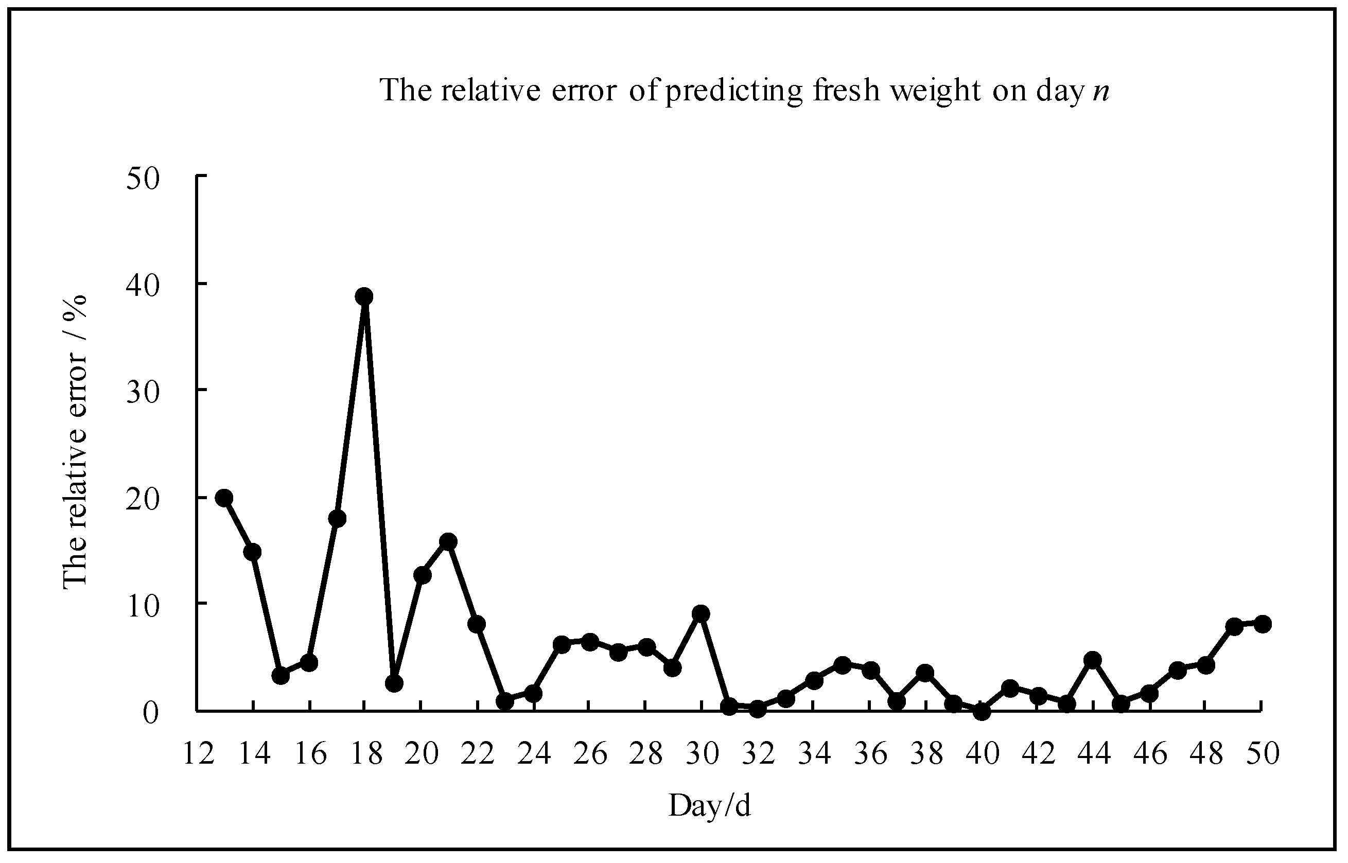
2.5.1. Predicting the Fresh Weight on the Next Day

Firstly, a dataset labeled 1 is constructed using instantaneous fresh weight, cumulative environmental factors, and fresh weight increment in the previous k days from day 1 to day n0, with a total of n0 − k elements. The dataset labeled 1 is imported into the naive Bayesian network for training and testing of the model. Then, instantaneous fresh weight on day n0 − k + 1 and cumulative environmental factors from day n0 − k + 1 to day n0 + 1 are taken as the inputs of the above model, and the fresh weight increment from day n0 − k + 1 to day n0 + 1 is derived by substituting the above model. Finally, the instantaneous fresh weight on day n0 + 1 is calculated and the relative error is calculated. The specific calculation formula is as follows:
m n 0 = m k + Δ m n 0 k
R E = | m n 0   m n 0 | m n 0
M R E = 1 n i = 1 n R E i        
σ = 1 n - 1 i = 1 n ( R E i M R E ) 2
where Δ m n 0 k is the predicted value of fresh weight increment from day n0 to day k (g),   m k is the measured value of instantaneous fresh weight on day k (g), m n 0 is the predicted value of instantaneous fresh weight on day n0 (g), m n 0 is the measured value of instantaneous fresh weight on day n0 (g), RE is the relative error between the predicted value and measured value of instantaneous fresh weight (%), MRE is the mean relative error (%), and σ is the standard deviation of relative error (%).

2.5.2. Predicting the Fresh Weight in the Next 2 Days

① Using the method of predicting the fresh weight on the next day, the fresh weight increment from day n0 − k − 1 to day n0 + 1 can be obtained.
② The instantaneous fresh weight on day n0 − k + 1, cumulative environmental factors, and predicted fresh weight increment from day n0 − k + 1 to day n0 + 1 are taken as the last element group to construct a new dataset labeled 2, with a total of n0 − k + 1 elements. The dataset labeled 2 is imported into the naive Bayesian network for training and testing of the model.
③ The cumulative environmental factors from day n0 − k + 2 to day n0 + 2 and the instantaneous fresh weight on day n0 − k + 2 are taken as the inputs of the above model, and the fresh weight increment from day n0 − k + 2 to day n0 + 2 is derived by substituting them into the above model.
④ With reference to Equations (13) and (14), the instantaneous fresh weight on day n0 + 2 and the relative error are calculated.

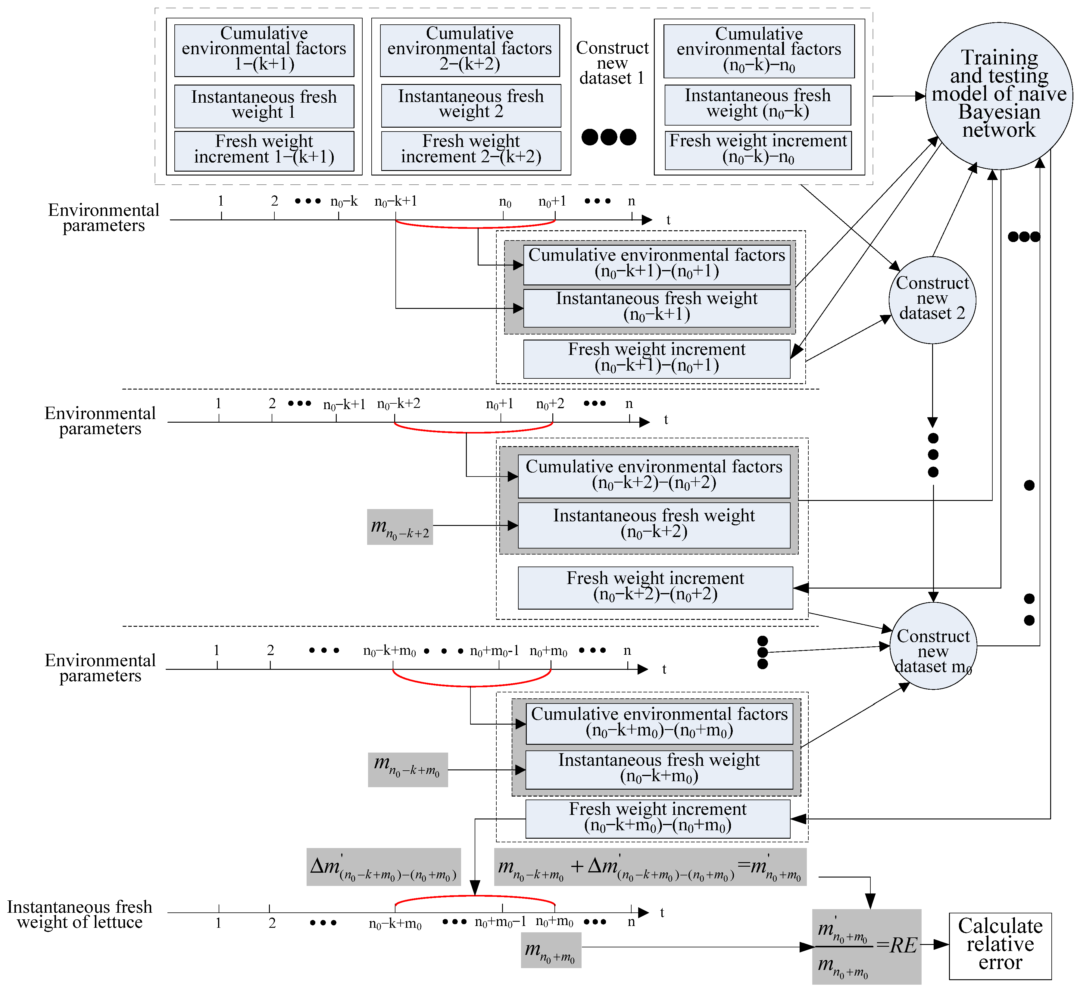
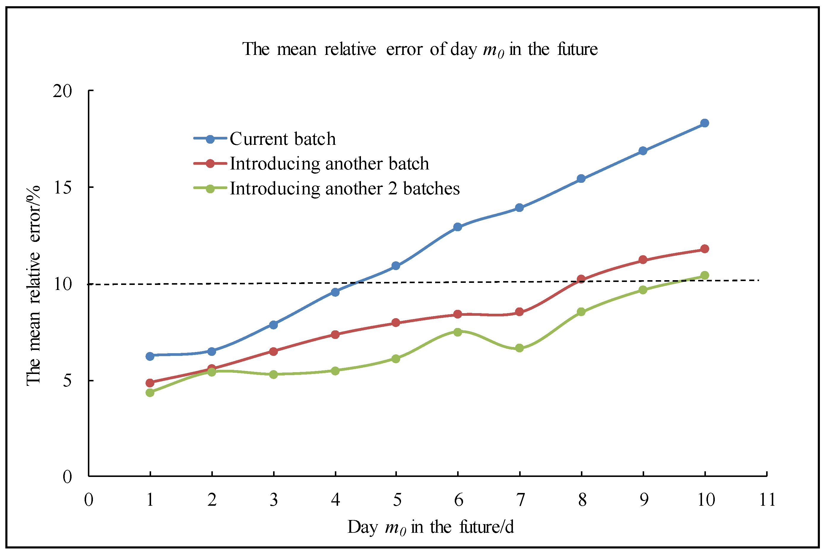
2.5.3. Predicting the Fresh Weight in the Next m0 Days

Schematic diagram of the solution process for predicting fresh weight in the next m0 days based on the phenotypic and environmental data from the previous k days is shown as Figure 4.
① According to the method of predicting the fresh weight in the next 2 days, the fresh weight increment from day n0 − k − 2 to day n0 + 2 can be obtained.
② By analogy, the instantaneous fresh weight on day n0 − k + m0 − 1, cumulative environmental factors, and predicted fresh weight increment from day n0 − k + m0 − 1 to day n0 + m0 − 1 are taken as the last element to construct a new dataset labeled m0, which has a total of n0 − k + m0 − 1 elements. The dataset labeled m0 is imported into the naive Bayesian network for training and testing of the model.
③ The cumulative environmental factors from day n0 − k + m0 to day n0 + m0 and the instantaneous fresh weight on day n0 + m0 are taken as the inputs of the above model, and the fresh weight increment from day n0 − k + m0 to day n0 + m0 is derived by substituting them into the above model.
④ With reference to Equations (13) and (14), the instantaneous fresh weight on day n0 + m0 and the relative error are calculated.
Therefore, through the above methods, the future fresh weight can be predicted using phenotypic and environmental data. For example, if instantaneous fresh weight on the next day is predicted, the cumulative environmental factors from day n0 − k + 1 to day n0 + 1 will be used, which from day n0 − k + 1 to day n0 are real and known. However, the cumulative environmental factors from day n0 to day n0 + 1 have not occurred and are unknown. Even if there is an error in estimating the environmental factors from day n0 to day n0 + 1, the impact on the accuracy of the cumulative environmental factors from day n0 − k + 1 to n0 + 1 is only 1/k. The overall error generated in fresh weight dynamic prediction is not too large.

3. Results and Discussion

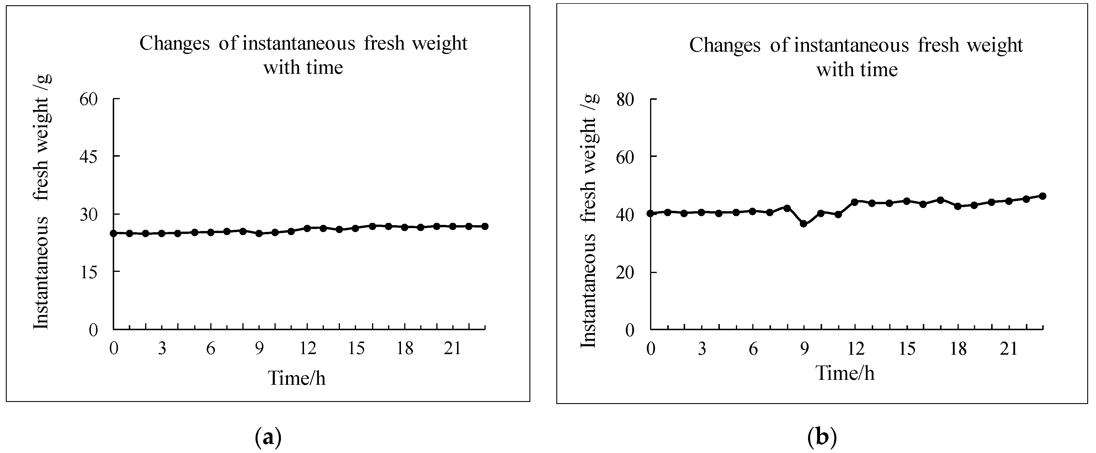
3.1. Fresh Weight Growth Curve of Lettuce

It can be seen from Figure 5 that on both sunny and cloudy days, the changes in fresh weight at nighttime are not obvious, while the changes in fresh weight during the daytime are relatively obvious. The fresh weight tends to decrease in the morning when the sun suddenly becomes stronger. The fresh weight then rises slowly and gradually recovers. When the sun is shining brightly at noon, the fresh weight tends to decrease again. The fresh weight recovers slowly in the afternoon, and it tends to remain stable. The main reason is that the transpiration during the daytime is obviously higher than that at nighttime [34], and the lettuce water content changes faster under the high temperatures, strong light, and low humidity of the daytime. Transpiration is an important indicator for measuring plant water content [35], and its strength is closely related to the degree of water loss in plants [36]. Moreover, water absorption through roots is the main way that water content is maintained in plants [37]. When the water lost by transpiration is higher than that absorbed by roots, the fresh weight of lettuce shows a downward trend. With the decrease of water content in a lettuce plant, a larger pull force is created, forcing the root to absorb more water to maintain normal metabolism and to supplement the water lost through transpiration. When the rate of water absorption by the roots increases slowly, approaching and exceeding the rate of water loss by transpiration, the fresh weight decreases slowly, stops gradually, and begins to increase. Finally, the fresh weight approaches the previous fresh weight range. During the processes of losing water through transpiration and absorption of water through the roots, and with the increase of photosynthesis of the lettuce leaves, the content of organic matter produced by photosynthesis gradually increases in the plant, making the lettuce larger in volume and allowing more water to be stored in the plant. The fresh weight of lettuce will then increase.
By comparing the change of fresh weight on a sunny day with that on a cloudy day, it was found that the variation in fresh weight growth on the sunny day was higher than that on the cloudy day. This was mainly due to the higher temperatures, stronger illumination, and lower humidity on the sunny day than on the cloudy day, meaning that the volumes of water lost through transpiration and absorbed by the roots were greater and the variations of fresh weight were stronger. There is no sunlight at nighttime and there is little change in temperature and humidity. The water lost by transpiration and the water absorbed by roots is relatively stable. At the same time, compared with a cloudy day, lettuce has a higher level of photosynthesis and accumulates more organic matter on a sunny day, which enables lettuce to absorb more water, increasing its fresh weight.
In order to accurately construct the relationship between the environmental factors and fresh weight growth, the calculation time of cumulative environmental factors and instantaneous fresh weight of lettuce was set at 8:00 AM.

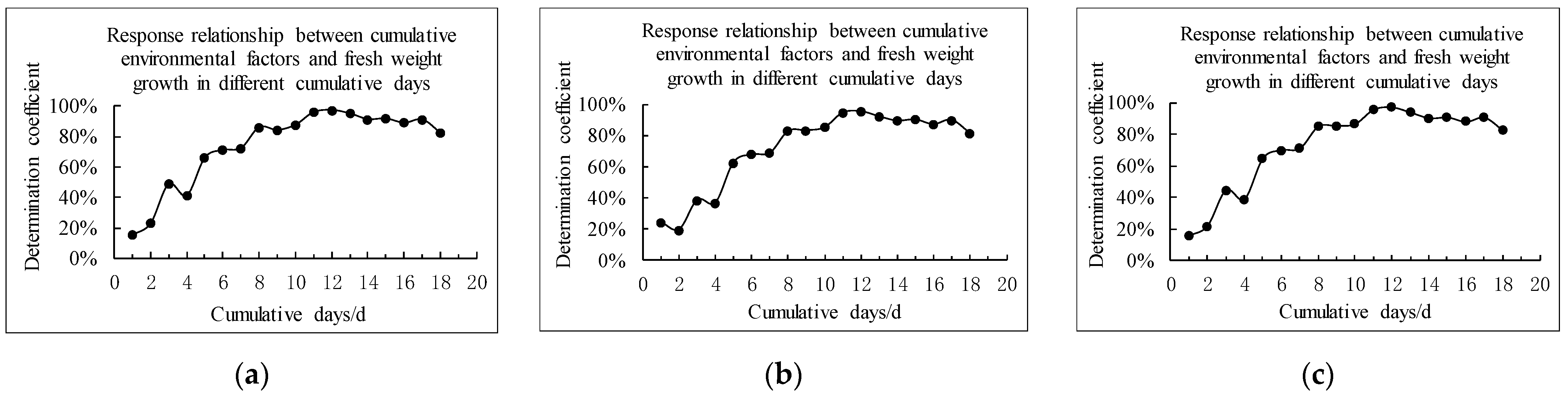
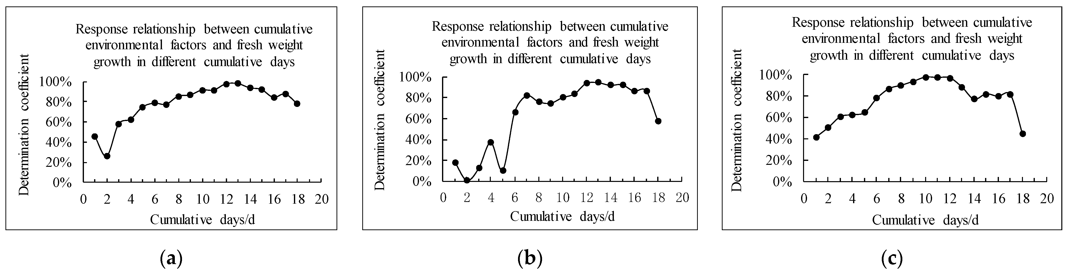
3.2. Optimum Response Time

It can be seen from Figure 6 that the response relationship between cumulative environmental factors and fresh weight growth over different cumulative days was different during the growth process among different samples in the same batch. With the increase in the number of cumulative days, the predicted determination coefficient showed a trend of increase at first. There was an individual decline in this process, but it did not affect the trend of increase. When the cumulative time reached 12 days, the determination coefficients for samples 1, 2, and 3 reached maximum values of 97.02%, 95.64%, and 97.06%, followed by a trend of decrease. In this process, there was an individual increase, but it did not affect the decreasing trend. The optimum response time of the most significant correlation between cumulative environmental factors and fresh weight growth among the different samples in the same batch was 12 days.
It can be seen from Figure 7 that the response relationship between cumulative environmental factors and fresh weight growth in different cumulative days was different during the growth process among the different samples in different batches. With the increase of cumulative days, the determination coefficient showed a trend of gradual increase at first. In this process, there was a decline in some cases, but it did not affect the trend of increase. When the determination coefficient reached the maximum value, it began to decrease. In this process, there was an increase in some cases, but it did not affect the decreasing trend. In the samples from the first batch, the coefficient of determination reached a maximum value of 97.57% for 13 cumulative days. The determination coefficient for 12 cumulative days was 97.29%, which was very close to the maximum value of the determination coefficient, and only 0.28% lower. In the samples of the second batch, the determination coefficient reached a maximum value of 94.14% for 13 cumulative days. The determination coefficient for 12 cumulative days was 93.47%, which was very close to the maximum value of the determination coefficient, and only 0.67% lower. In the samples of the third batch, the determination coefficient reached a maximum value of 97.72% for 10 cumulative days. The determination coefficient for 11 cumulative days was 97.39%, which was very close to the maximum value, and only 0.33% lower. The determination coefficient for 12 cumulative days was 97.09%, which was very close to the maximum value, and only 0.63% lower.
It can be seen in Table 1 that with the increasing number of cumulative days, the average value of the determination coefficient in the three batches of samples showed a trend of first increasing and then decreasing. When the cumulative time reached 12 days, the average of the determination coefficient reached its maximum value of 95.95%, indicating that the optimum response time of the most significant correlation between cumulative environmental factors and fresh weight growth among different samples in the different batches was 12 days.

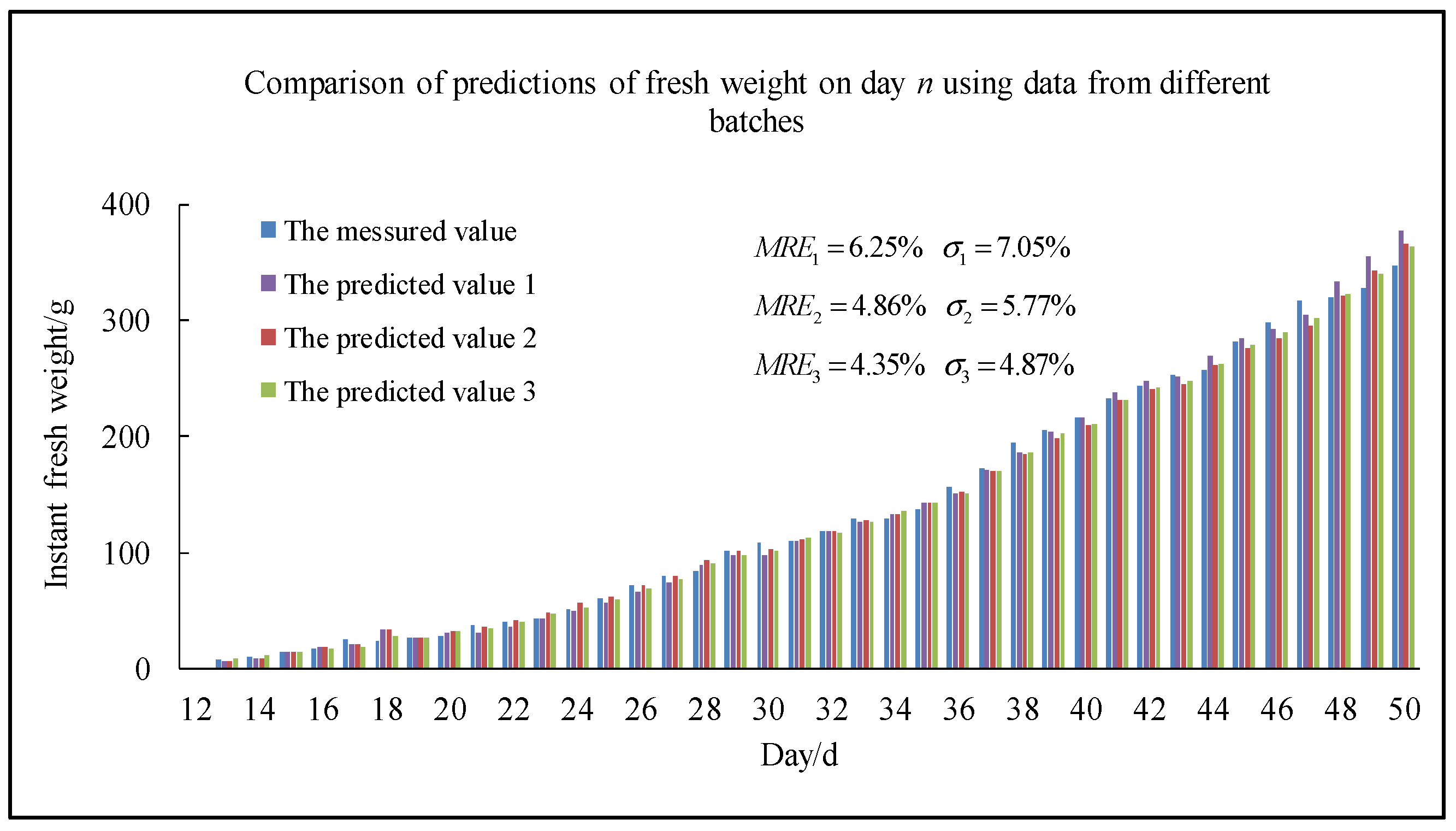
3.3. Using Batch Data to Predict the Dynamic Fresh Weight of Lettuce

It is obvious from Figure 8 that the fresh weight on the next day can be predicted by using only the data from the current batch (MRE1 = 6.25%, σ1 = 7.05%). The relative error (Figure 9) of predicting fresh weight using only the data from the current batch fluctuated greatly at first, and there was one point with a relative error of 40.9%. Subsequently, the relative error fluctuation began to stabilize. This is mainly because the number of elements constructed from the data of the current batch was relatively small at the initial stage, and the accuracy of the model trained by the naive Bayesian network was relatively low. With the increase of the number of elements in the dataset, the accuracy of the model trained by the naive Bayesian network gradually improved, and the relative error started to decrease.
It can be seen from Table 2 that only the data from the current batch were used to predict fresh weight, and the relative error gradually increased with the increasing number of future days (MRE: 6.25% < 6.50% < 7.88%, σ: 7.05% < 6.76% < 11.17%). The data from the current batch with the introduction of another batch were used to predict fresh weight, and the relative error had a tendency to increase with the increasing number of future days (MRE: 4.86% < 5.57% < 6.50%, σ: 5.77% < 6.04%, 5.77% < 5.78%). The data from the current batch with the introduction of another two batches were used to predict fresh weight, and the relative error gradually increased with the increasing number of future days (MRE: 4.35% < 5.40% < 5.29%, σ: 4.87% < 5.38% < 6.11%).
As shown in Figure 10, the data from the current batch were used to predict the fresh weight in the future. With the increasing number of future days, the MRE of fresh weight prediction gradually increased. In other words, the accuracy of predicting fresh weight in the future gradually decreased, and the MRE of fresh weight prediction over 4 days based on data from the current batch was not more than 9.57%.
Upon introducing another batch of data, the MRE of fresh weight prediction gradually increased with the increasing number of future days. However, it was lower than that of the fresh weight predicted using only the data from the current batch, and the MRE of fresh weight prediction in the next 7 days based on the introduction of another batch of data was not more than 8.53%, indicating that the accuracy of predicting fresh weight was improved by introducing another batch.
After introducing the data from another two batches, the MRE of fresh weight prediction tended to increase with increasing number of future days. However, it was lower than that for the fresh weight predicted using the data with only one additional batch, and the MRE of fresh weight prediction over 9 days based on the introduction of data from another two batches was not more than 9.68%, indicating that the accuracy of the fresh weight prediction could be further improved by introducing more batches.

4. Conclusions and Future Work

A dynamic fresh weight growth prediction model based on phenotypic and environmental batch data was proposed, and was used to predict the dynamic fresh weight growth of substrate-cultivated lettuce in a solar greenhouse under normal water and fertilizer conditions. The computation of cumulative environmental factors and instantaneous fresh weight of batches of lettuce was achieved. The optimum response days were explored through the most significant correlations between cumulative environmental factors and fresh weight growth. A dynamic fresh weight prediction model was established using a naive Bayesian network based on cumulative environmental factors, instantaneous fresh weight, and fresh weight increments of batches. Experimental results showed that the calculation time setpoint of cumulative environmental factors and instantaneous fresh weight of lettuce was 8:00 AM and the optimum response time was 12 days. The MRE of fresh weight prediction over 4 days based on data from the current batch was not more than 9.57%; upon introducing another batch of data, the prediction over 7 days dropped to not more than 8.53% MRE; upon introducing another two batches, the prediction over 9 days dropped to not more than 9.68% MRE, proving the model’s feasibility.
In future work, the proposed dynamic growth prediction model of fresh weight will be integrated with an automatic management system and sensing data to support an autonomous fertigation strategy for substrate-cultivated leafy vegetables in a solar greenhouse system, playing an important role in promoting the automatic cultivation and management of vegetables in agricultural applications.

Author Contributions

L.L.: writing—original draft, conceptualization, methodology, investigation, data curation, software, and validation. J.Y.: writing—review and editing, conceptualization, and funding acquisition. X.W.: investigation. X.L.: writing—review and editing, formal analysis, funding acquisition, and project administration. L.G.: writing—review and editing, funding acquisition, project administration. All authors have read and agreed to the published version of the manuscript.

Funding

This research was supported by the National Natural Science Foundation of China (52275262), and the Shanghai Science and Technology Innovation Action Plan Project (21N21900100).

Institutional Review Board Statement

Not applicable.

Informed Consent Statement

Not applicable.

Data Availability Statement

Anyone can access the data by sending an email to jyuan@sdau.edu.cn.

Conflicts of Interest

The authors declare no conflict of interest.

References

  1. Kalkhajeh, Y.K.; Huang, B.; Hu, W.; Ma, C.; Gao, H.; Thompson, M.L.; Hansen, H.C.B. Environmental soil quality and vegetable safety under current greenhouse vegetable production management in China. Agric. Ecosyst. Environ. 2021, 307, 107230. [Google Scholar] [CrossRef]
  2. Sun, Z.; You, L.; Muller, D. Synthesis of agricultural land system change in China over the past 40 years. J. Land Use Sci. 2019, 13, 473–479. [Google Scholar] [CrossRef] [Green Version]
  3. Chen, C.; Yu, N.; Yang, F.; Mahkamov, K.; Han, F.; Li, Y.; Ling, H. Theoretical and experimental study on selection of physical dimensions of passive solar greenhouses for enhanced energy performance. Sol. Energy 2019, 191, 46–56. [Google Scholar] [CrossRef]
  4. Wang, H.Y.; Zu, G.; Yang, F.J.; Li, D.Z.; Tian, L.M. Design of multi-functional solar greenhouses in high latitude areas. Trans. CSAE 2020, 36, 170–178. [Google Scholar]
  5. Bao, E.C.; Cao, Y.F.; Zou, Z.R.; Shen, T.T.; Zhang, Y. Research progress of thermal storage technology in energy-saving solar greenhouse. Trans. CSAE 2018, 34, 1–14. [Google Scholar]
  6. Nemali, K. History of Controlled Environment Horticulture: Greenhouses. HortScience 2022, 57, 239–246. [Google Scholar] [CrossRef]
  7. Berkers, E.; Geels, F.W. System innovation through stepwise reconfiguration: The case of technological transitions in Dutch greenhouse horticulture (1930–1980). Technol. Anal. Strateg. Manag. 2011, 23, 227–247. [Google Scholar] [CrossRef]
  8. Wang, T.; Wu, G.; Chen, J.; Cui, P.; Chen, Z.; Yan, Y.; Zhang, Y.; Li, M.; Niu, D.; Li, B.; et al. Integration of solar technology to modern greenhouse in China: Current status, challenges and prospect. Renew. Sustain. Energy Rev. 2017, 70, 1178–1188. [Google Scholar] [CrossRef]
  9. Koukounaras, A. Advanced Greenhouse Horticulture: New Technologies and Cultivation Practices. Horticulturae 2021, 7, 1. [Google Scholar] [CrossRef]
  10. Lin, D.; Zhang, L.; Xia, X. Model predictive control of a Venlo-type greenhouse system considering electrical energy, water and carbon dioxide consumption. Appl. Energy 2021, 298, 117163. [Google Scholar] [CrossRef]
  11. Yu, G.; Zhang, S.; Li, S.; Zhang, M.; Benli, H.; Wang, Y. Numerical Investigation for Effects of Natural Light and Ventilation on 3D Tomato Body Heat Distribution in a Venlo Greenhouse. Inf. Process. Agric. 2022, in press. [Google Scholar] [CrossRef]
  12. Liu, W. Engineering Technology Development of Temperature and Lighting Control Promote Productivity of Chinese Solar Greenhouse. Agric. Eng. 2015, 5, 15–17+42. [Google Scholar]
  13. Rajasekar, M.; Arumugam, T.; Kumar, S.R. Influence of weather and growing environment on vegetable growth and yield. J. Hort. 2013, 5, 160–167. [Google Scholar]
  14. Hang, T.; Lu, N.; Takagaki, M.; Mao, H. Leaf area model based on thermal effectiveness and photosynthetically active radiation in lettuce grown in mini-plant factories under different light cycles. Sci. Hortic. 2019, 252, 113–120. [Google Scholar] [CrossRef]
  15. Zhang, L.; Xu, Z.; Xu, D.; Ma, J.; Chen, Y.; Fu, Z. Growth monitoring of greenhouse lettuce based on a convolutional neural network. Hortic. Res. 2020, 7, 124. [Google Scholar] [CrossRef] [PubMed]
  16. Chang, C.-L.; Chung, S.-C.; Fu, W.-L.; Huang, C.-C. Artificial intelligence approaches to predict growth, harvest day, and quality of lettuce (Lactuca sativa L.) in a IoT-enabled greenhouse system. Biosyst. Eng. 2021, 212, 77–105. [Google Scholar] [CrossRef]
  17. Graamans, L.; Baeza, E.; Dobbelstena, A.; Tsafaras, I.; Stanghellini, C. Plant factories versus greenhouses: Comparison of resource use efficiency. Agric. Syst. 2018, 160, 31–43. [Google Scholar] [CrossRef]
  18. Kocian, A.; Massa, D.; Cannazzaro, S.; Incrocci, L.; Di Lonardo, S.; Milazzo, P.; Chessa, S. Dynamic Bayesian network for crop growth prediction in greenhouses. Comput. Electron. Agr. 2020, 169, 105167. [Google Scholar] [CrossRef]
  19. Yanes, A.R.; Martinez, P.; Ahmad, R. Real-time growth rate and fresh weight estimation for little gem romaine lettuce in aquaponic grow beds. J. Comput. Electron. Agric. 2020, 179, 105827. [Google Scholar] [CrossRef]
  20. Jung, D.-H.; Park, S.H.; Han, H.; Kim, H.-J. Image processing methods for measurement of lettuce fresh weight. J. Biosyst. Eng. 2015, 40, 89–93. [Google Scholar] [CrossRef] [Green Version]
  21. Jiang, J.-S.; Kim, H.-J.; Cho, W.-J. On-the-go image processing system for spatial mapping of lettuce fresh weight in plant factory. IFAC-PapersOnLine 2018, 51, 130–134. [Google Scholar] [CrossRef]
  22. Liu, Z.G.; Wang, J.Z.; Xu, Y.F.; Li, P.P. Lettuce yield and root distribution in substrates under drip irrigation and micro-sprinkler irrigation. Trans. Chin. Soc. Agric. Mach. 2014, 45, 156–160. [Google Scholar]
  23. Chen, X.L.; Yang, Q.C.; Ma, T.G.; Xue, X.Z.; Qiao, X.J.; Guo, W.Z. Effects of red and blue LED irradiation in different alternating frequencies on growth and quality of lettuce. Trans. Chin. Soc. Agric. Mach. 2017, 48, 257–262. [Google Scholar]
  24. Liu, L.; Yuan, J.; Zhang, Y.; Liu, X.M. Non-destructive Estimation Method of Fresh Weight of Substrate Cultured Lettuce in Solar Greenhouse. Trans. Chin. Soc. Agric. Mach. 2021, 52, 230–240. [Google Scholar]
  25. Bian, Z.H.; Yang, Q.C.; Liu, W.K. Effects of light quality on the accumulation of phytochemicals in vegetables produced in controlled environments: A review. J. Sci. Food Agric. 2015, 95, 869–877. [Google Scholar] [CrossRef]
  26. Zhou, T.M.; Zhen, W.; Wang, Y.C.; Su, X.J.; Qin, C.X.; Huo, H.Q.; Jiang, F.L. Modelling seedling development using thermal effectiveness and photosynthetically active radiation. J. Integr. Agric. 2019, 18, 2521–2533. [Google Scholar] [CrossRef]
  27. Gu, Z.; Yuan, S.Q.; Qi, Z.M.; Wang, X.K.; Cai, B. Real-time precise irrigation scheduling and control system in solar greenhouse based on ET and water balance. Trans. Chin. Soc. Agric. Mach. 2018, 34, 101–108. [Google Scholar]
  28. Allen, R.G.; Pereira, L.; Raes, D.; Smith, M. Crop Evapotranspiration-Guidelines for Computing Crop Water Requirements. In FAO Irrigation and Drainage Paper 56; FAO: Rome, Italy, 1998. [Google Scholar]
  29. Mao, J.X. Analysis on conversion between solar radiance and illuminance. J. Henan Agric. Sci. 1995, 240, 11–12. [Google Scholar]
  30. Li, X.; Luo, X.L.; Wang, R.; Li, T.L.; Xu, H.; Zhao, X.Y. Analysis on Solar Radiation’s Changing Laws and Utilization in Solar Greenhouse. Chin. Agric. Sci. Bull. 2012, 28, 104–108. [Google Scholar]
  31. Langarizadeh, M.; Moghbeli, F. Applying naive bayesian networks to disease prediction: A systematic review. Acta Inform. Med. 2016, 24, 364. [Google Scholar] [CrossRef]
  32. Li, L.X.; Rahman, S.S.A. Students’ learning style detection using tree augmented naive Bayes. R. Soc. Open Sci. 2018, 5, 172108. [Google Scholar] [CrossRef] [PubMed] [Green Version]
  33. Harzevili, N.S.; Alizadeh, S.H. Mixture of latent multinomial naive Bayes classifier. Appl. Soft Comput. J. 2018, 69, 516–527. [Google Scholar] [CrossRef]
  34. Resco de Dios, V.; Roy, J.; Ferrio, J.P.; Alday, J.G.; Landais, D.; Milcu, A.; Gessler, A. Processes driving nocturnal transpiration and implications for estimating land evapotranspiration. Sci. Rep. 2015, 5, 10975. [Google Scholar] [CrossRef] [PubMed]
  35. Maes, W.H.; Steppe, K. Estimating evapotranspiration and drought stress with ground-based thermal remote sensing in agriculture: A review. J. Exp. Bot. 2012, 63, 4671–4712. [Google Scholar] [CrossRef] [PubMed] [Green Version]
  36. Adeyemi, O.; Grove, I.; Peets, S.; Domun, Y.; Norton, T. Dynamic modelling of lettuce transpiration for water status monitoring. Comput. Electron. Agric. 2018, 155, 50–57. [Google Scholar] [CrossRef]
  37. Jackson, R.B.; Sperry, J.S.; Dawson, T.E. Root water uptake and transport: Using physiological processes in global predictions. Trends Plant Sci. 2000, 5, 482–488. [Google Scholar] [CrossRef]
Figure 1. Lettuce cultivation experiment.
Agriculture 12 01959 g001
Figure 2. Schematic diagram of calculation of instantaneous fresh weight.
Agriculture 12 01959 g002
Figure 3. Schematic diagram of the solution process for the most significant response between cumulative environmental factors and fresh weight growth in the previous k days.
Agriculture 12 01959 g003
Figure 4. Schematic diagram of the solution process for predicting fresh weight in the next m0 days based on the phenotypic and environmental data from the previous k days.
Agriculture 12 01959 g004
Figure 5. Fresh weight growth curves in different weather conditions. (a) On a cloudy day, (b) on a sunny day.
Agriculture 12 01959 g005
Figure 6. The response relationship between cumulative environmental factors and fresh weight growth among the different samples in the same batch. (a) Sample 1, (b) sample 2, (c) sample 3.
Agriculture 12 01959 g006
Figure 7. The response relationship between cumulative environmental factors and fresh weight growth among the samples in different batches. (a) Samples from the first batch, (b) samples from the second batch, (c) samples from the third batch.
Agriculture 12 01959 g007
Figure 8. Prediction of fresh weight on the next day. Note: Predicted value 1 is the value of fresh weight on the next day predicted using the data of the current batch. Predicted value 2 is the value of fresh weight on the next day predicted by introducing another batch. Predicted value 3 is the value of fresh weight on the next day predicted by introducing the data from another 2 batches.
Agriculture 12 01959 g008
Figure 9. The relative error of predicting fresh weight using only the data from the current batch.
Agriculture 12 01959 g009
Figure 10. Comparison chart of the mean relative error of predicted future fresh weight.
Agriculture 12 01959 g010
Table 1. Numerical distribution table of adjacent regions with maximum values of the coefficient of determination in different batches.
Cumulative DaysFirst Batch SamplesSecond Batch SamplesThird Batch SamplesAverage
100.91170.79760.97720.8955
110.91220.83390.97390.9067
120.97290.93470.97090.9595
130.97570.94140.88660.9346
Table 2. Prediction of fresh weight error over the next 3 days.
ErrorDay 1 in the FutureDay 2 in the FutureDay 3 in the Future
BatchesMREσMREσMREσ
Current batch6.25%7.05%6.50%6.76%7.88%11.17%
Introducing another batch4.86%5.77%5.57%6.04%6.50%5.78%
Introducing another 2 batches4.35%4.87%5.40%5.38%5.29%6.11%
Publisher’s Note: MDPI stays neutral with regard to jurisdictional claims in published maps and institutional affiliations.

