Deep Learning Ensemble-Based Automated and High-Performing Recognition of Coffee Leaf Disease

Abstract

Coffee is the world’s most traded tropical crop, accounting for most export profits, and is a significant source of income for the countries in which it is produced. To meet the needs of the coffee market worldwide, farmers need to increase and monitor coffee production and quality. Coffee leaf disease is a significant factor that decreases coffee quality and production. In this research study, we aim to accurately classify and detect the diseases in four major types of coffee leaf disease (phoma, miner, rust, and Cercospora) in images using deep learning (DL)-based architectures, which are the most powerful artificial intelligence (AI) techniques. Specifically, we present an ensemble approach for DL models using our proposed layer. In our proposed approach, we employ transfer learning and numerous pre-trained CNN networks to extract deep characteristics from images of the coffee plant leaf. Several DL architectures then accumulate the extracted deep features. The best three models that perform well in classification are chosen and concatenated to build an ensemble architecture that is then given into classifiers to determine the outcome. Additionally, a data pre-processing and augmentation method is applied to enhance the quality and increase the data sample’s quantity to improve the training of the proposed method. According to the evaluation in this study, among all DL models, the proposed ensemble architecture outperformed other state-of-the-art neural networks by achieving 97.31% validation. An ablation study is also conducted to perform a comparative analysis of DL models in different scenarios.

1. Introduction

Coffee is the most traded tropical crop, with up to 25 million farming households contributing up to 80% of the worldwide output. Coffee production is concentrated in developing nations, where it accounts for a substantial portion of the export profits and is a primary source of revenue. It is one of the world’s most popular drinks and is among the most traded commodities [1], where the market is continuously growing owing to increased demand in emerging economies and its substantial contribution to specialized and innovative products in developed countries. The diseases affecting coffee plants are a critical factor severely limiting coffee’s productivity. Biotic stresses, such as leaf miner, rust, phoma, and Cercospora, damage coffee plants and cause defoliation and a reduction in photosynthesis, thus reducing the production and quality of the product [2]. Thus, identifying and measuring plant diseases is highly important in phytopathology. It is essential to understand both causal agents and the severity of the symptoms for effective pest and disease management [3]. If not treated appropriately, these diseases can cause significant leaf damage and crop fatality [4].

The Fourth Industrial Revolution (4IR) is the peak era of current industrial technology, where cyber–physical systems can be connected via deep learning, machine learning, artificial intelligence, and big data [5]. The 4IR can also increase productivity and growth in various aspects. One of the sectors experiencing technological growth and development is agriculture, where technologies such as artificial intelligence, machine learning, and deep learning positively impact agriculture’s development and productivity [6]. Smart agriculture is a new and evolving technology that integrates advanced strategies for increasing agricultural production while also increasing agricultural inputs in a sustainable and environmentally responsible manner. It is now possible to reduce errors and expenses to achieve ecologically and economically sustainable agriculture [7]. Recently, several efforts have been made to use artificial intelligence (AI) to help farmers accurately recognize diseases and pests that damage agricultural production and to judge the severity of the symptoms.

AI attempts to provide computers with human-like intelligence by simulating human intelligence processes. It allows for analysis, learning, and problem solving while presenting new knowledge. AI has the potential to transform agriculture by allowing farmers to obtain better results with less work while providing numerous additional benefits [8]. In recent years, AI research has experienced significant growth in machine learning applications, particularly a new class of models called deep learning. Notably, DL algorithms have demonstrated better performance in various domains than traditional machine learning methods [9,10]. DL models have significant relevance when promising outcomes are obtained. Many methods have been used in recent years to identify diseases in plants, and DL methods have proven to be quite efficient. Owing to the growing interest in DL in agriculture, numerous studies have been conducted, demonstrating that visual evaluation is reliable for plant disease detection [11]. Researchers have been developing DL solutions for agriculture in recent years by classifying species and diseases using convolutional neural networks (CNN) [12,13]. CNNs are the most promising DL-based algorithms for automatically discriminating features and learning robustness. DL consists of several convolutional layers representing learning features based on data [14].

However, DL has drawbacks, such as the necessity of large amounts of data for training the network. For example, the performance of the CNN deteriorates if the available dataset does not contain sufficient images. This critical drawback can be overcome via transfer learning. Transfer Learning has several advantages, one of which is that it does not require a large amount of data for training the network, as knowledge from previous similar learning tasks can be transferred to the current task. The control of crop losses is ensured by the rapid recognition of the disease’s cause, which enables the prompt selection of the best protective strategy. It also represents the initial and most crucial phase of disease prevention. Our motivation is to develop a system that can adequately classify coffee diseases. Early disease identification can result in more successful treatments and longer survival spans. Although transfer learning has been used in several disease detection methods [15,16,17,18,19], researchers need to develop more disease detection methods in coffee plants using transfer learning.

Herein, relevant works on machine learning and deep learning for classifying and detecting plant diseases are reviewed. Marcos et al. [20] focused on detecting rust in coffee leaves. This study used a genetic algorithm to compute an optimal convolution kernel mask that emphasizes fungal infections’ texture and color features. Gutte et al. [21] used three phases for monocot and dicot diseases. First, they segmented the leaf using the k-mean clustering technique. Feature extraction was then performed to determine the shape, color, and texture. Finally, they used a support vector machine (SVM) to identify plant diseases. Abrham et al. [22] classify coffee leaf disease into three major types of disease: Coffee Wilt Disease (CWD), Coffee Berry Disease (CBD), and Coffee Leaf Rust (CLR). First, the author used GLCM and color features for feature extraction; then, they used an artificial neural network (ANN), k-Nearest Neighbors (KNN), a Naïve and a hybrid self-organizing map (SOM), and a Radial basis function (RBF) for classifying the coffee plant leaf diseases.

Manso et al. [23] proposed an application for detecting coffee leaf diseases in images captured using smartphones. Various types of backgrounds for images using the YCbCr (Luminance, Chrominance) and HSV (Hue, Saturation, Value) color spaces were analyzed throughout the segmentation process and compared with k-means clustering in the YCbCr color space. The iterative threshold algorithm is called the Otsu algorithm and calculates the damage caused by coffee plant diseases. Finally, for a classification in the segmentation of foliar damage, an ANN trained with a robust machine learning algorithm was used. According to the experts, the result obtained is auspicious, as it shows the feasibility and effectiveness of identifying and classifying foliar damage. Babu et al. [24] developed a software model that effectively suggests corrective measures for disease or pest management in the agricultural field and achieves control solutions. They used five modules. First, they extracted the edge of a leaf to find the token value. Second, the module trained the neural network with the leaf and identified the error graph. Identifying and recognizing the leaf disease or pest species was carried out during the third and fourth modules. The last module attempted to match the identified disease or pest samples to examples in the database containing disease and pest image samples and suggest appropriate actions.

Marcos et al. [25] proposed training a CNN for identifying rust infection. For an evaluation, they provided a set of images to an expert. The author compared the results, which showed that the method could recognize infection with high precision, as evidenced by the high dice coefficient. Dann et al. [26] used the YOLOv3-MobileNetv2 model for detecting diseases in robusta coffee leaves. They develop a prototype that can capture the input images and then classify the disease into four classes: Cercospora, miner, phoma, and rust. Ramcharan et al. used a smartphone-based CNN model to identify cassava plant diseases with an accuracy rate of 80.6% [27].

In [28], transfer learning was used to classify ten diseases in four major crops that have received little attention. The data were transferred from a smartphone to a computer through a local area network (LAN), and the performances of six pre-trained CNNs, i.e., GoogLeNet, VGG19, DenseNet201, VGG-16, AlexNet, and ResNet101, were evaluated. GoogLeNet had the best validation accuracy at 97.3%. Real-time image classification was performed under the test conditions, and the prediction scores for each disease class were obtained. All models showed a reduction in accuracy, with VGG-16 achieving the highest accuracy at 90%. Esgario et al. [29] used 1747 images of Arabica leaf and trained various deep convolutional models (VGG-16 and ResNet50) for classifying the degree of severity and biotic stress. The trained VGG-16 DCNN, which identified various biotic diseases, achieved a 95.47% accuracy, whereas ResNet50 validated each leaf condition efficiently with a 95.63% accuracy rate.

In the literature, although significant efforts have been made to develop various DL models to identify diseases in several crops, these models, unfortunately, are neither feasible nor effective for detecting coffee disease. Therefore, a reliable approach is needed to accurately identify various diseases in coffee plants. To satisfy this need, we propose a DL-based ensemble architecture in this paper, which yields efficient and accurate results.

Table 1. Detailed analyses of the proposed and state-of-the-art studies.

Reference	Model	Strength	Weakness
[20]	Genetic Algorithm	- Superior performance to Otsu segmentation method - Obtained high dice coefficient score	- Ineffective control over luminosity inhomogeneity - Small dataset
[21]	Support Vector Machines	- Post-processing not required - Better results on instance segmentation	- High computational cost - Excessive pre-processing required
[23]	Extreme Learning Machine	- Automatic detection using the mobile application - Great results from an extreme learning machine	- The image results from the camera’s automatic adjustment are different - Need more segmentation adjustment for background color
[24]	Deep Convolutional Networks	- Able to detect 13 different types of diseases - Big impact augmentation process	- Small dataset - Fine-tuning does not have a big impact
[25]	Convolutional Neural Network	Simple morphology erosion improves the detection	Has a long runtime
[26]	YOLOv3-MobileNetv2	- Lightweight depth-wise convolutions are used - Good lighting conditions	- Has a long runtime - High computational cost
[27]	Single-Shot Multibox (SSD) with MobileNet	- Good results of detection boxes - Model inference time is quite fast	- Decrease in model recall - Decrease in performance from image to video
[28]	ResNet101, VGG16, DenseNet201, GoogLeNet, AlexNet, and VGG19	- A cost-effective resources system - Transmitted data using Local Area Network (LAN)	- Decrease in accuracy results on real-time classification - Unstable Internet/LAN network
[29]	A Multi-task System Based on CNN	- Using multi-task on the CNN model - Low cost	- Low dataset representation - Has a long runtime
Ours	Ensemble Learning Technique	- Improved accuracy over prior techniques - Robust to noise and better generalization	- Extensive training is required - Relies on large data

shows the detailed analyses of the state-of-the-art studies and our proposed model. In this paper, we, for the first time, develop fine-tuned and high-performing deep CNNs for coffee leaf disease detection (or classification) using transfer learning and conduct an extensive experimental optimization of the constructed CNNs. The main contributions of our work are as follows:

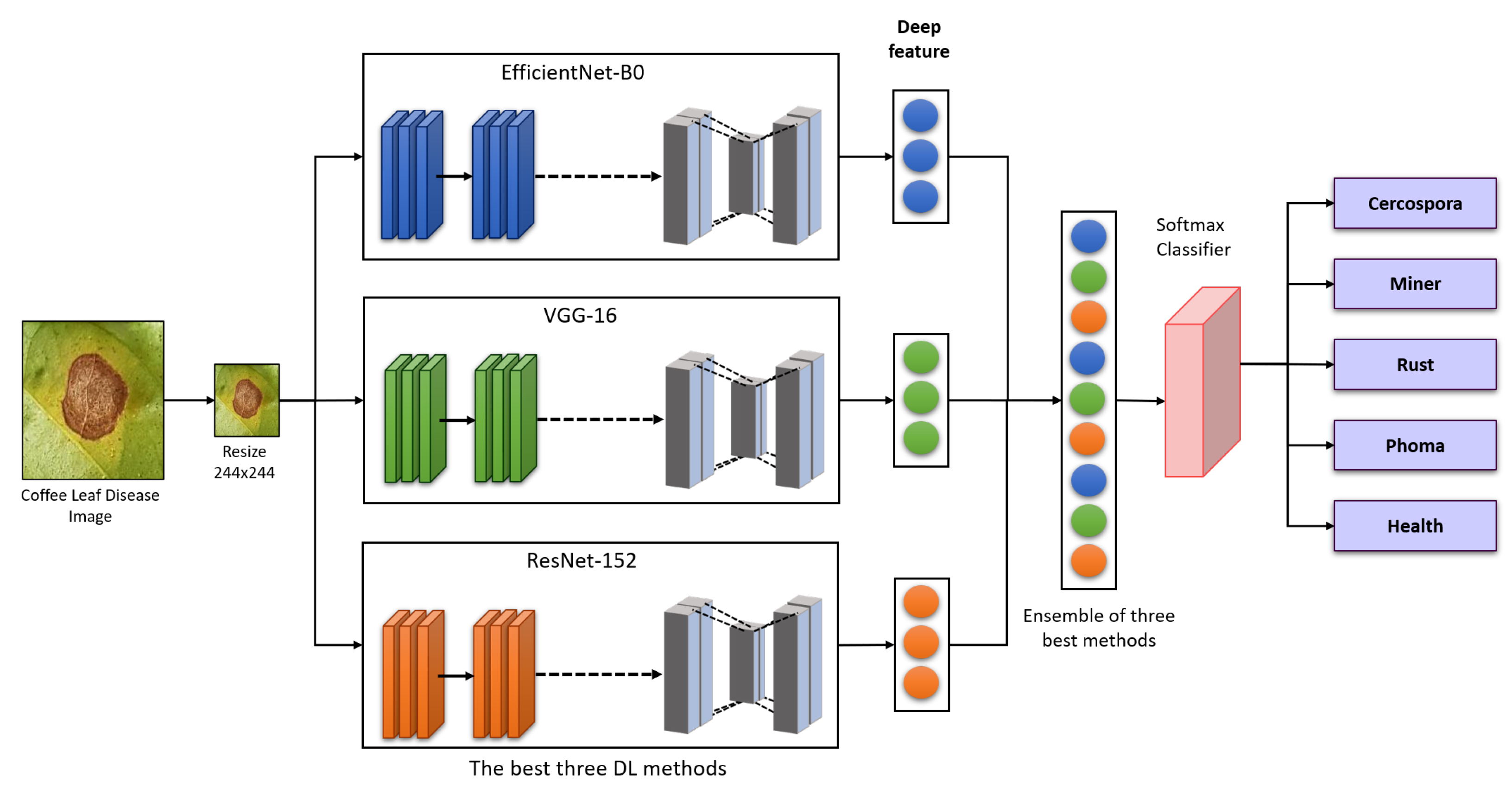
• We develop a collaborative ensemble architecture to classify the diseases in coffee plants. The proposed strategy is based on re-training the pre-trained DL models using the coffee disease dataset and combining the weights of the three best-performing algorithms to make an ensemble architecture for better disease detection in coffee leaf.
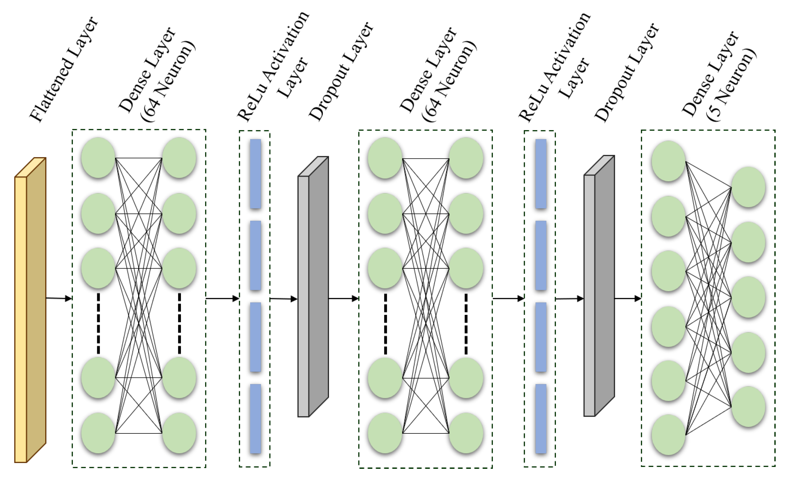
• The pre-trained DL models utilized in this study are fine-tuned using our proposed layers, which can replace traditional disease detection in plants and improve overall classification accuracy.
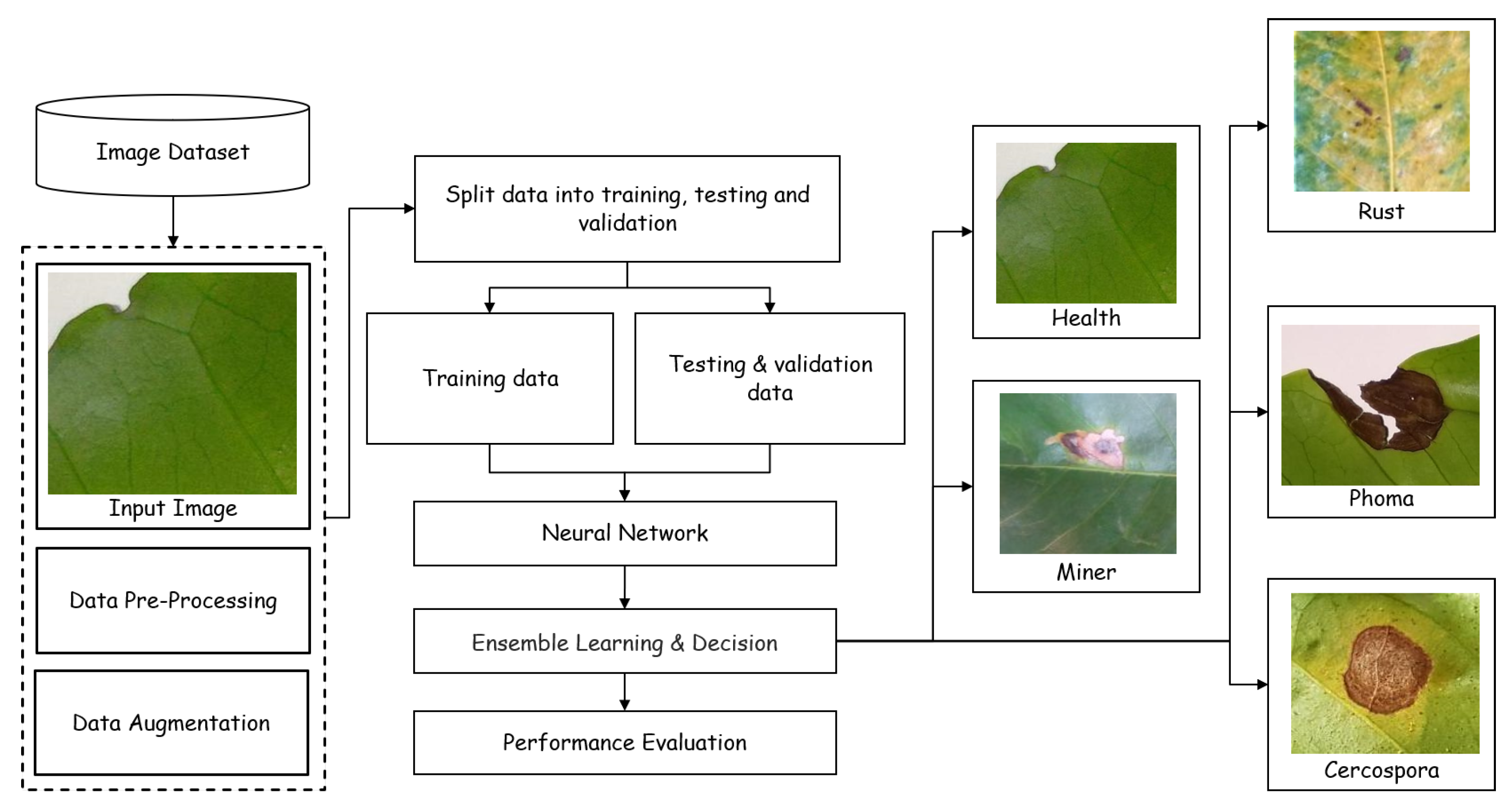
• A data pre-processing and data augmentation strategy is employed to improve the poor image quality of the training data and increase the diversity in input data to generate better outcomes on small datasets.
• The effectiveness of the proposed architecture is assessed with several hyper-parameters such as activation functions, batch size, learning rate, and L2 regularizer, to increase classification accuracy. This ablation study demonstrates how our architecture outperforms the previous state-of-the-art studies in detecting coffee leaf diseases.

The remainder of this paper is organized as follows: In Section 2, the materials and methods are described. The experimental results are described and compared with those of other recent iterative methods in Section 3. Finally, future studies and conclusions are described in Section 4.

2. Materials and Methods

This section thoroughly discusses the proposed method with pre-trained algorithms, multiple layers, and ensemble learning. An illustration of the pre-processing, augmentations, training, and evaluation stages of coffee leaf disease identification is shown in Figure 1. DL algorithms are trained and optimized using a variety of hyper-parameters for fine-tuning and transfer learning methods. In neural networks, optimizers adjust the learning rates and biases accordingly. In the ensemble stage, we finally combine the three best DL methods to increase the accuracy of the results.

2.1. Ensemble Method

In this study, we implement an ensemble method by combining the three best models to improve the classification accuracy rate for solving the problem of coffee leaf disease detection and classification. The ensemble method usually produces more accurate results than a single model. One of the standard techniques for generating ensemble-based algorithms is bagging. Bagging is a practical and straightforward method to improve performance. It involves two steps: the first is applying the base model to the training dataset, and the second step is aggregating the generated models by combining the predictions from several predictors. Our ensemble method architecture is shown in Figure 2, which combines EfficientNet-B0, ResNet-152, and VGG-16, which are the best three DL models under consideration. The ensemble learning we used can be represented by the following equation:

$$f\left(Y\right)=\sum _{i=1}^n{w}_k{f}_i\left(Y\right)$$

(1)

where Y is a model input vector, n is the number of models, $f\left(Y\right)$ is the aggregated model predictor, $w_k$ is the aggregating weight for combining the ith model, and $f_i\left(X\right)$ is the ith model. The standard error predictions are used as an indicator of model prediction confidence, which is given by:

$${\sigma }_e={\{\frac{1}{n-1}\sum _{b=1}^n{[y(x_j;W^b)-y(x_j;·)]}^2\}}^{1/2}$$

(2)

where $y(x_j;.)={\sum }_{b=1}^{n}y(x_j;W^b)/n$, and n is the number of neural networks. The associated model prediction is more reliable if ${\sigma }_e$ is smaller. We adopt DL models by fine-tuning the last layers through transfer learning and layer freezing. The images are resized and augmented to $224\times 224\times 3$; subsequently, they are fed into a pre-trained model for automatic feature extraction.

In this study, we adopt EfficientNet-B0, ResNet-152, VGG-16, InceptionV3, Xception, MobileNetV2, DenseNet 201, InceptionResNetV2, and NasNetMobile for our recommended layer. For the CNN-based model, the output can be represented by:

$$X_K^L=f\left(\sum _{i\in M_k}{X}_K^{L-1}\ast W_{lk}^L+b_K^L\right)$$

(3)

The final layer comprises two dropout layers, three fully connected layers, a flattening layer, and a softmax classifier generated from the base models. Due to the flattened layer, we direct and convert the feature sets from the last layer into a 1D array, which is then passed into a dense layer containing 64 hidden units. We used ReLu for the activation function, which is given by:

$$f\left(x\right)=max(0,x)$$

(4)

where x is output of each neuron.

Figure 3 represents our proposed layer. A rectified linear unit function is used before the prediction process to activate the dense layer, representing a label with one neuron. This method uses a linear approach, in which biases and weights are applied to each feature map to generate the probability. We use a 20% dropout rate in the dropout layer to eliminate overfitting in the hidden layer with 64 hidden neurons. For our final classifier, we use the softmax function [30], which is given by:

$$\sigma {(\overrightarrow{\mathrm{z}})}_i=\frac{e^{z_i}}{{\sum }_{j=1}^K{e}^{z_i}}$$

(5)

where $\overrightarrow{\mathrm{z}}$ denotes the input vector, $z_i$ represents the elements of the input vector, and K denotes the total number of classes.

EfficientNet-B0 generates different CNN-family models using a composite scaling method. This series is approximately six times faster and eight times smaller than other deep neural networks such as VGG-16, Inception-V3, ResNet-152, and DenseNet201. The network depth is determined by the number of layers in the network. The number of filters in the convolutional layer determines its depth. The resolution is determined by the width and height of the input image. ResNet-152 is a CNN model developed by Kaiming et al. [31]. ResNet-152 contains 152 layers, three layers for each residual function, and has the highest accuracy among the Resnet family members. VGG-16 is a CNN usually recognized as one of the best computer vision models [32]. This model significantly improved prior-art configurations, evaluated the networks, and increased the depth using a minimal ($3\times 3$) convolution filter architecture consisting of 16 convolutional layers. Figure 4, represents the overall architectures with proposed layers used to classify coffee leaf diseases.

2.2. Fine Tuning and Transfer Learning

In this section, we explain how to train and fine-tune our model. First, in the pre-trained base model, we use the ImageNet dataset weights, obtained using 14 million images classified into 1000 categories. These weights can be imported from the Keras library. The base models trained on ImageNet weights can quickly utilize available features and improve their image recognition performance due to their pre-initialized weights. Image classification features are included in ImageNet’s weights, which are obtained through training. Compared with randomly selected weights, the transfer learning process reduces the amount of work required, and it accelerates [33] the process while requiring less work than arbitrarily initialized weights. Second, using a coffee leaf disease image as training data, we fine-tuned our proposed end layers by freezing the other layers of all base models. As a result, the above-specified technique used in training prevents the initial layers of models from being overwritten by the coffee dataset weights during the initial training epochs. Thus, we can preserve the initial pre-trained ImageNet weights in the initial layer for better training purposes. After the model’s final layers are trained with our coffee dataset, the entire network is unfrozen, where the classifier and our proposed layers are then integrated and constructed our proposed model using weights from the ImageNet dataset as well as the coffee leaf disease image dataset. Our test data are used in the final validation of our model.

2.3. Loss Function and Hyper-Parameter

This section describes how these loss functions and hyper-parameters are chosen to produce an efficient approach to solving the problem. Both loss and accuracy determine the performance of a deep learning model [34,35]. As DL models aim for the lowest possible error rate, a model will be more efficient if the computed loss is lower than if the computed loss is higher. For multi-class classification, we use categorical cross-entropy to calculate the average difference between the expected value, the predicted value, and the loss measurement. The categorical cross-entropy is given by,

$$L_{\left(CCE\right)}=\sum _{q=1}^l{y}_q\ast log\left({\widehat{y}}_q\right)$$

(6)

where ${\widehat{y}}_q$ denotes the i scalar value in the model output, $y_q$ denotes the equivalent target value, and the output size is the number of scalar values in the model’s output. The local minima can be quickly approached by weights using an adaptive gradient descent function during the training process. To achieve the most outstanding results from loss reduction, a better learning process, efficient memory use, and implementation simplicity, we select the Adam optimizer over other optimization algorithms, such as RMSProp or SGD [36];

Table 2. Validation accuracy achieved using Adam, SGD, and RMSProp optimizers.

Models	Adam	SGD	RMSProp
VGG-16	94.2	93.1	93.9
Inception-V3	83.9	83.8	78.6
ResNet-152	93.8	93.8	90.3
Xception	85.4	85.1	85.3
MobileNet-V2	74.6	64.6	74.5
DenseNet	83.8	83.7	84.6
InceptionResNet-V2	86.9	85.8	86.7
NASNetMobile	83.8	82.3	81.5
EfficientNet-B0	95	91.9	94.23

shows that Adam achieves better results than SGD and RMSProp. Small learning rates (LR) are presented for the hyper-parameter values and are shown in

Table 3. Loss function and Hyper-parameters.

No.	Hyper-Parameters	Values
1	Reduced LR	$10e^{-5}$
2	Initial LR	$10e^{-3}$
3	Optimizer	Adam
4	Loss function	Categorical cross-entropy
5	Epoch	50
6	Batch size	32

. The Adam optimizer achieves rapid convergence with greater efficiency and speed. To avoid overloading computational memory when sending information over a network, we use a batch size of 32. Furthermore, each model is trained for 50 epochs with a fixed duration to observe the reaction.

2.4. Dataset

This study uses five classes for classification: healthy, phoma, miner, rust, and Cercospora. Explanations for each class are presented in

Table 4. Detailed class dataset.

Type of Leaf	Description
Healthy	Green without any spots or damage of any kind.
Miner (Peri Leucoptera coffee)	Large, wavy dark patches on the leaf’s upper surface. Rubbing an area or bending a leaf causes the upper epidermis to break, revealing tiny white caterpillars in the new mines.
Phoma (Phoma costaricensis)	A leaf that turns brown and dies starting from the tip area.
Cercospora (Cercospora coffeicola)	Dry areas that are brown in color with a border in the shape of a bright halo around it.
Rust (Hemileia vastatrix)	Features patches that resemble a halo that ranges in color from yellow to brown.

. The dataset contains 1300 images, consisting of 260 images for each class. We divided the dataset evenly between the five classes, with 20% used for validation and 80% used for training. All sample images are resized and normalized using Keras’s automatic resizing script, which resizes all input images to 224 × 224 in dimensions because no two images have the exact same dimensions. The image dataset used in this experiment is the same as that used in the symptom dataset in Esgario’s study [29]. We use images as a subset and make minor modifications by keeping the number of classes the same. The dataset that we use has a large number of disease images, and the images of diseases are shown more clearly. Additionally, there are no image duplications in the dataset that we use.

2.5. Data Preprocessing and Augmentation

The data are transformed into a standard classification format after pre-processing the images. The images are first converted into RGB, and the pixel resolution is kept constant at 224 × 224 pixels. As part of the image augmentation process, an open-source Keras ImageDataGenerator class is used to enhance the dataset size by recreating images using various pre-processing techniques, including random rotation (15°), horizontal and vertical flips, width and height shifts, shear ranges, fill modes, and transpositions. The Keras normalization function is used to normalize the images of coffee leaf diseases, which transforms the input images’ floating pixel values.

2.6. Experimental Setup

In experimentation, we use Python with the Keras and TensorFlow frameworks for fine-tuning our model. During training, the network was implemented on a computer with a 2.60 GHz Intel Core i5-11400 CPU. An NVIDIA RTX A5000 GPU was used with a 64-bit operating system and 16 GB of RAM to conduct the experiments. The details are presented in

Table 5. System requirements.

No.	Name	Parameter
1	Development tool	Python 3.7
2	CPU	Intel Core i5-11400, 2.60 GHz
3	GPU	Nvidia RTX A5000 GDDR6 24 GB
4	Memory	16 GB
5	Library	TensorFlow
6	System type	Windows 10, 64 bit

. The pre-trained network was imported from Keras, and the first layer of the base model is frozen in the first stage. The entire network is retrained using a fine-tuning network based on the proposed layer and the coffee leaf disease images. We compare the proposed CNN model with several other CNN models to validate our results. Some of the validation procedures used for the dataset in this study are discussed in Section 3.

2.7. Performance Evaluation Metrics

A confusion matrix, also known as an error matrix, describes the performance of a classification model with a set of test data. A confusion matrix can be used to calculate the potential of the classifier. All diagonal elements indicate that the outcomes were correctly classified. The unclassified results are represented in the off-diagonals of the confusion matrix. Consequently, the ideal classifier will have a confusion matrix with only diagonal elements, with the other elements set to zero. Following the categorization procedure, a confusion matrix provides actual and expected values [37]. There are rows and columns in the confusion matrix (CM) that correspond to the ground truth labels and the actual class (e.g., healthy, phoma, miner, rust, or Cercospora). A similar prediction value is provided for each validation sample, representing the number of incorrect and correct classifications or predictions. A true positive is defined as the percentage of correctly identified positive samples classified as positive. In contrast, a true negative is defined as the percentage of negative samples correctly classified as negative. When an image is identified as positive but is actually negative, this is known as a false positive. A false negative is a result that appears to be positive but is actually negative [38]. Various metrics were used to assess the DL-based models’ performances, including the precision, F1 score, area under the receiver operating characteristic (ROC) curve, validation accuracy, recall, specificity, and sensitivity. The following Equations (7)–(11) are used to calculate the F1-score, precision, specificity, accuracy rate, and sensitivity of each model:

$$Precision=\frac{TP}{TP+FP},$$

(7)

$$F1-Score=\frac{2\left(TP\right)}{2\left(TP\right)+FP+FN}.$$

(8)

$$Specificity=\frac{TN}{TP+FN},$$

(9)

$$Accuracy=\frac{TN+TP}{TN+TP+FN+FP},$$

(10)

$$Sensitivity=\frac{TP}{FN+TP},$$

(11)

3. Results and Discussion

A publicly accessible dataset is used to evaluate the performance of the proposed technique [29]. We used the symptom dataset as the subset, and the dataset is categorized into five classes, where four classes are coffee leaf diseases (miner, phoma, Cercospora, rust,) and one class contains healthy leaves. This dataset yields a significant amount of heterogeneous agricultural data (containing 1300 images). This dataset is used in the training and testing process. For model development, we utilize EfficientNet-B0, ResNet-152, VGG-16, InceptionV3, Xception, MobileNetV2, DenseNet 201, InceptionResNetV2, and NasNetMobile with several data pre-processing and augmentation techniques to increase the size and diversity of the images. We employ an Adam optimizer in our optimization technique, which has been widely used in previous investigations, with an initial learning rate of 0.001 and a learning rate drop component of 0.1. For instance, the training learning rate dropped to 0.0001 ($0.001\times 0.1$) after 10 iterations, to 0.00001 ($0.0001\times 0.1$) after 20 epochs, etc. For the other hyper-parameter used in this study, we used a mini-batch of 32 and the cross-entropy loss function. Simultaneously, we use Keras and TensorFlow APIs to develop fine-tuned baseline architectures. The proposed architectures are trained using 20% of the test data and 80% of the training data. The hyper-parameters included in this design plan show that the accuracy improved gradually as the number of epochs increased over a short period, stabilizing at a given amount.

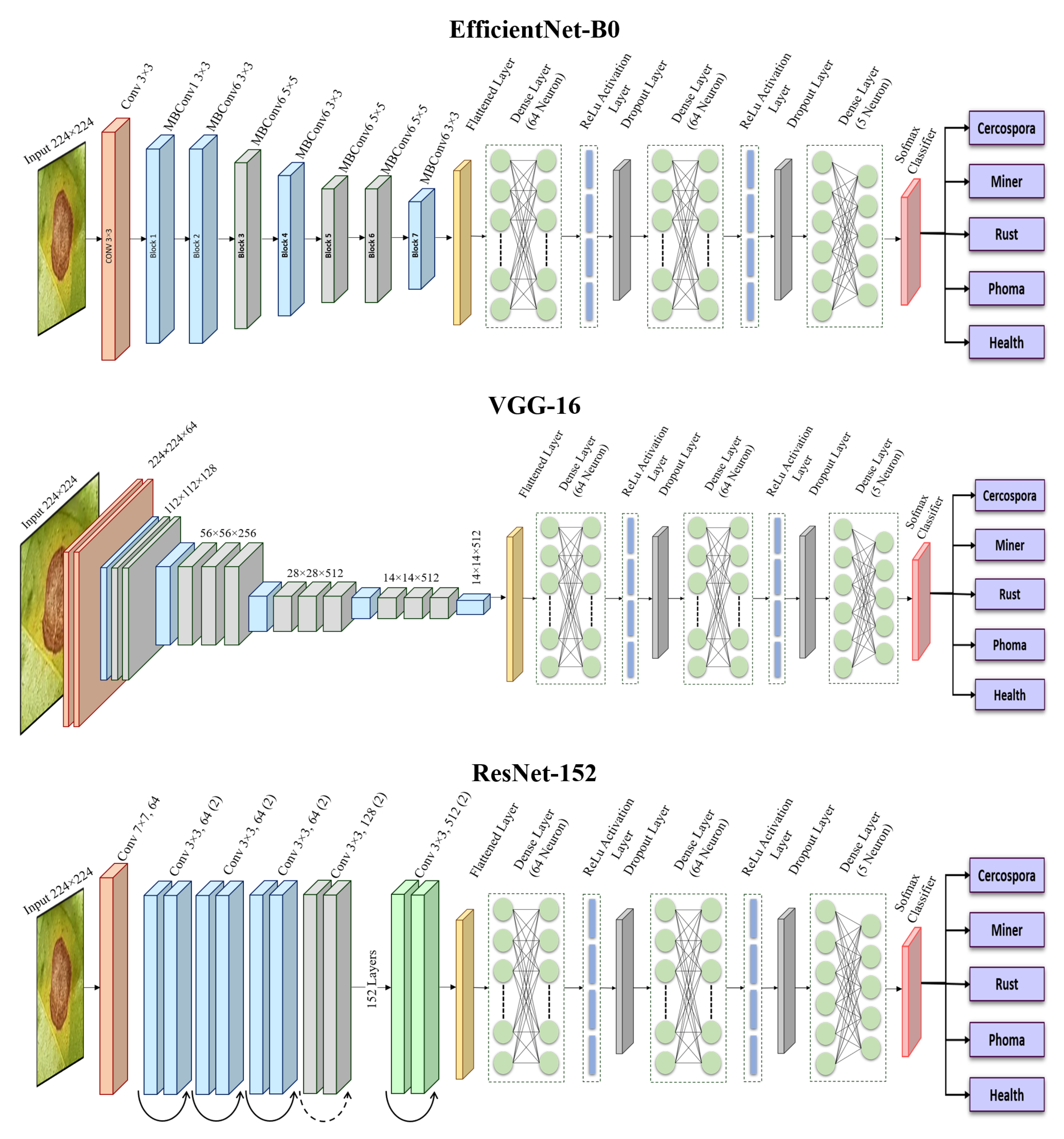
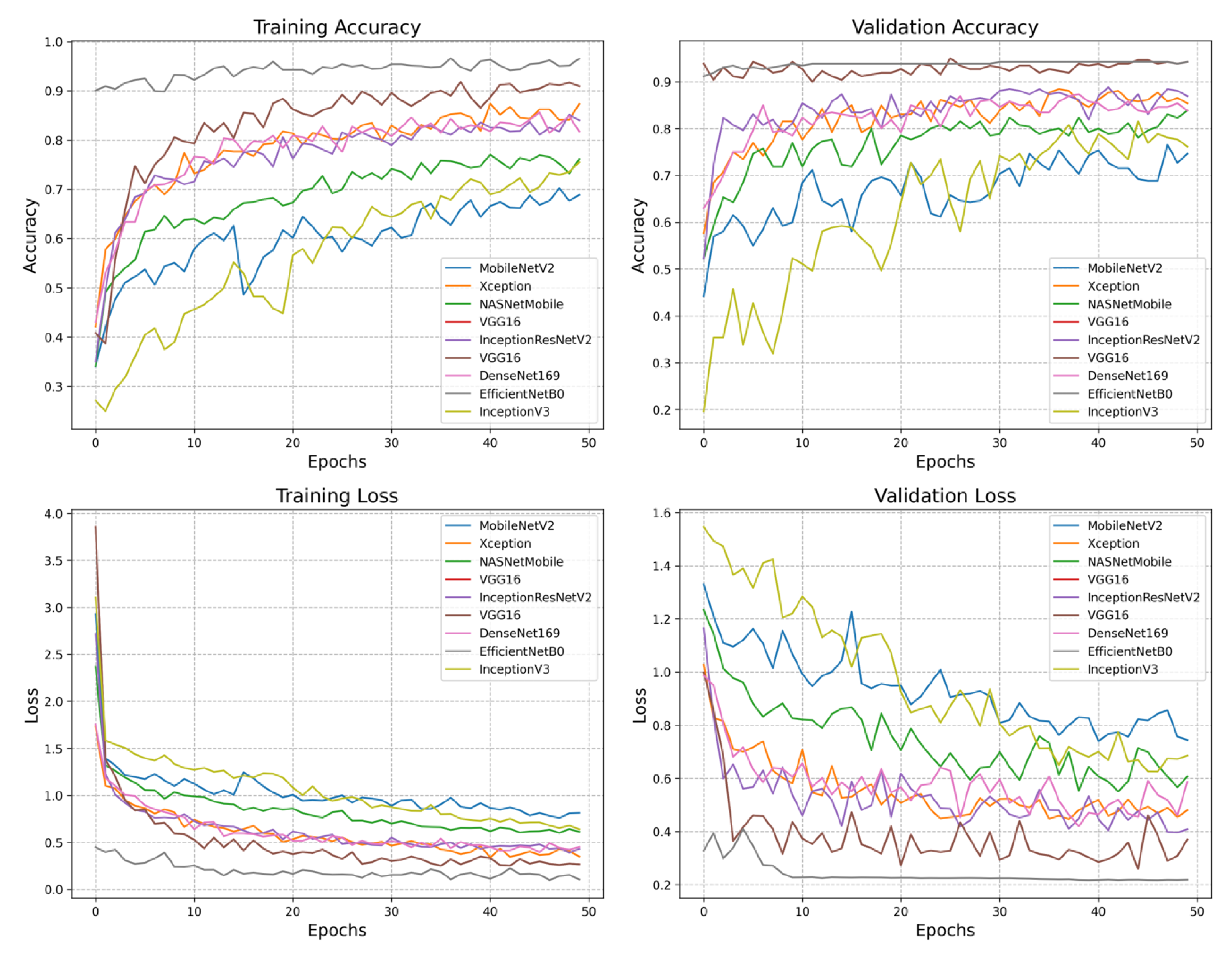
Figure 5 shows the graph of accuracy and loss in training and validation. In the training accuracy graph, EfficientNet-B0 and VGG-16 perform very well, achieving more than 90% accuracy. The last model is MobileNet-V2, achieving a less than 70% error rate. With a minimum loss, EfficientNet-B0 shows the highest validation accuracy of 95%. VGG-16 performed well on the coffee leaf dataset, achieving 94.2% validation accuracy. The ResNet-152 architecture achieves satisfactory performance with 93.8% validation accuracy, while MobileNet-V2 shows a low performance with 74.6% validation accuracy. Overall, EfficientNet-B0 performs very well, followed by VGG-16 in training and validation loss accuracy. Finally, MobileNet-V2 demonstrates poor performance in training and validation loss accuracy.

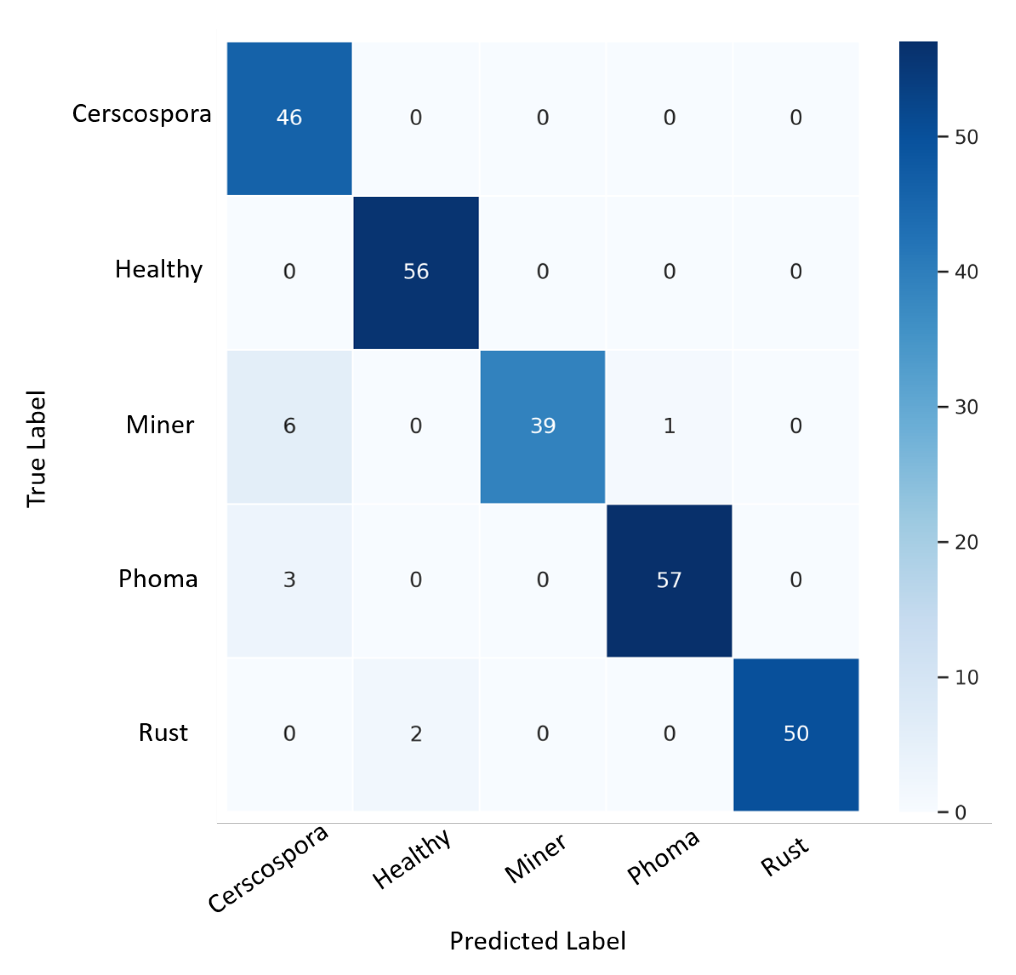
A total of 248 images were validated in their respective classes using confusion matrix techniques.

Table 6. Performance comparison between the ensemble model and other fine-tuned models. PR = Precision; SN = Sensitivity; SP = Specificity; F1 = F1-Score; ACC = Accuracy.

Models	PR%	SN%	SP%	F1%	ACC%
VGG-16	94.4	94	98.6	94.1	94.2
Inception-V3	83.5	85.1	96.3	83.5	83.9
ResNet-152	94	93.2	98.5	93.3	93.8
Xception	85.5	85.3	96.6	85.2	85.4
MobileNet-V2	76.8	74.1	94.5	73.5	74.6
DenseNet	84.7	83.2	96.3	83.3	83.8
InceptionResNet-V2	86.7	86	97	86.1	86.9
NASNetMobile	85.1	83.1	96.3	83.3	83.8
EfficientNet-B0	95.2	94.8	98.8	94.9	95
Ensemble Model (ours)	95.7	95.2	98.9	95.1	97.3

presents the ensemble model’s and proposed model’s performance scores. The ensemble model achieves the highest state-of-the-art performance by achieving 97.3% in accuracy, 95.1% in F1-score, 98.9% in specificity, 95.2% in sensitivity, and 95.7% in precision. Next is the EfficientNet-B0 model, achieving 95% in accuracy, 94.9% in F1-score, 98.8% in specificity, 94.8% in sensitivity, and 95.2% in precision. VGG-16 follows, achieving 94.2% in accuracy, 94.1% in F1-score, 98.6% in specificity, 94% in sensitivity, and 94.4% in precision. Next is ResNet-152, achieving 93.8% in accuracy, 93.3% in F1-score, 98.5% in specificity, 93.2% in sensitivity, and 94% in precision. The MobileNet-V2 model achieves the lowest state-of-the-art performance by achieving 74.6% in accuracy, 73.5% in F1-score, 94.5% in specificity, 74.1% in sensitivity, and 76.8% in precision. Figure 6 presents the confusion matrix obtained by the proposed ensemble architecture on the validation dataset.

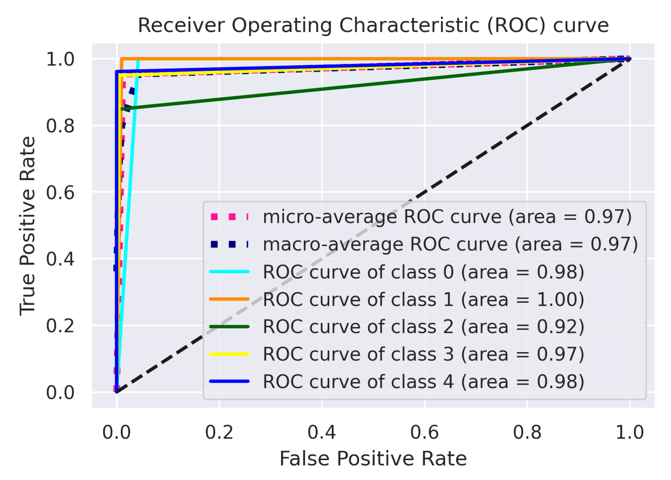
The area under the ROC graph is a measurable statistic for classification tasks with multiple threshold levels. An ROC curve is used for all potential thresholds to compare the true positive (sensitivity) against the false positive rate (1—specificity). The area under the curve (AUC) represents the degree of distinction. In contrast, the ROC is a probability graph. This indicates the effectiveness of the algorithm in discriminating between different classes. The model is more effective at differentiating between classes with diseased and healthy individuals with a higher AUC. Figure 7 illustrates the graph of the ensemble model, which shows that the ensemble outperforms the other architectures by correctly classifying the five different classes.

Table 7. Comparison of the AUC values for proposed ensemble architecture with other fine-tuned DL models. The classes 0, 1, 2, 3, 4 represent Cercospora, Healthy, Miner, Phoma, and Rust, respectively.

Models	Class 0	Class 1	Class 2	Class 3	Class 4	Micro-Average	Macro-Average
DenseNet	0.90	0.89	0.83	0.95	0.91	0.90	0.90
NASNetMobile	0.91	0.89	0.83	0.96	0.90	0.90	0.90
InceptionResNet-V2	0.85	0.97	0.84	0.92	0.98	0.92	0.91
MobileNet-V2	0.94	0.82	0.81	0.95	0.67	0.84	0.84
Xception	0.95	0.90	0.86	0.91	0.92	0.91	0.91
Inception-V3	0.86	0.74	0.83	0.93	0.88	0.85	0.85
VGG-16	0.97	0.97	0.95	0.98	0.95	0.96	0.96
Resnet-152	0.98	0.99	0.90	0.97	0.97	0.96	0.96
Efficientnet-B0	0.98	0.99	0.93	0.96	0.98	0.97	0.97
Ensemble (ours)	0.98	1.00	0.92	0.97	0.98	0.97	0.97

shows the ROC–AUC curve for the other fine-tuned models, where EfficientNet-B0 performs most satisfactorily by achieving a 0.97 macro-average score; the VGG-16 model trained with the coffee leaf disease dataset achieves a score of more than 0.96 for the macro-average score; ResNet-152 performs relatively well, achieving 0.96 macro- and micro-AUC scores; and MobileNet-V2 performs the worst among all the models by achieving a 0.84 macro-average score. Among all five classes, it scores lower for class 2 (miner), with only 0.86; the highest is class 3 (phoma), achieving 0.95 on average.

Table 8. Average Epoch time of the training and testing of the proposed ensemble architecture and other fine-tuned models.

Models	Average Train Time	Average Test Time
VGG-16	8 s	1 s
Inception-V3	8 s	23 ms
ResNet-152	9 s	1
Xception	8 s	1 s
MobileNet-V2	8 s	20 ms
DenseNet	8 s	43 ms
InceptionResNet-V2	8 s	1 s
NASNetMobile	8 s	34 ms
EfficientNet-B0	8 s	24 ms
Ensemble model (ours)	6.3 s	1 s

shows the performance time of our proposed ensemble architecture and other fine-tuned models. This table shows that our proposed ensemble architecture is faster than other fine-tuned models, achieving 6.3 s in the training process.

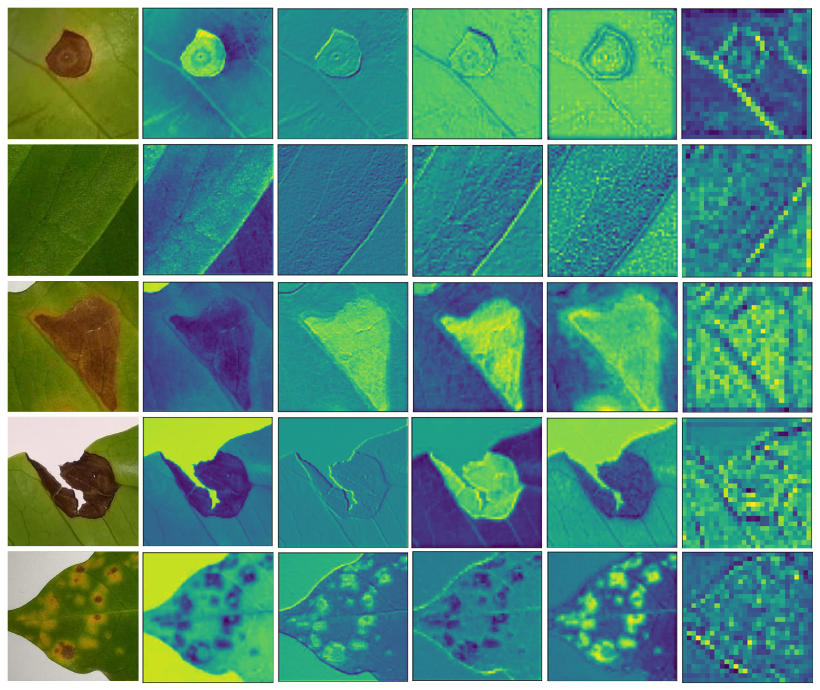
DL algorithms are very complex and are referred to as black boxes since any justification does not support the prognosis. The visual prediction presentation is essential for establishing confidence in AI-based intelligent systems. Figure 8 presents a visualization of images with feature maps extracted from the intermediate convolution layers of the ensemble model with different classes. Here, the model’s feature extraction capability as the convolutional network becomes deeper, from left to right, is presented. These feature maps show that the proposed network is effectively tuned to distinguish between diseases in coffee leaves. The first image is Cercospora, the second image is Healthy, the third image is miner, the fourth image is phoma, and the fifth image is rust. This section defines the size and number of features of the various fine-tuned CNN architectures used in this study. The CNNs and regular neural networks are identical. They consist of neurons with biases and weights that can be used for training. Each neuron processes a few impulses to conduct a dot product and may potentially perform non-linearity. In general, the parameters are weights that are learned through an activity. These include weighted vectors, which are modified during the backpropagation process and help the algorithm’s ability to anticipate outcomes.

Table 9. Parameters of the fine-tuned models.

Models	Parameters (M)
VGG-16	14
Inception-V3	21
ResNet-152	58
Xception	20
MobileNet-V2	2
DenseNet	12
InceptionResNet-V2	54
NASNetMobile	4
EfficientNet-B0	4

shows the parameter of the fine-tuned models used in this study. The best models that achieve higher accuracy are VGG-16 with 14 million parameters, EfficientNet-B0 with 4 million parameters, and ResNet-152 with 58 million parameters.

4. Conclusions

Coffee leaf diseases contribute to the decrease in quality in coffee production, and detecting these diseases is highly advantageous and offers a practical, easy, and appropriate way to improve coffee production. In this study, we proposed an effective and enhanced ensemble architecture based on EfficientNet-B0, ResNet-152, and VGG-16 to identify coffee leaf diseases. The proposed ensemble method achieved a maximum performance of 97.31% validation accuracy. Although this study applied nine transfer learning models and designs to identify coffee leaf disease, further research is still needed. In the future, we will develop more in-depth CNN techniques that detect coffee leaf diseases, e.g., by improving the detection and segmentation time efficiency and increasing the number of coffee leaf disease images in the dataset utilized in this study. The proposed method will be applied to various agricultural images for plant disease classification, fruit ripening detection, and cropland surveillance, providing a foundation for future studies.

References

1. Voora, V.; Bermúdez, S.; Larrea, C. Global Market Report: Coffee; IISD: Winnipeg, MB, Canada, 2019. [Google Scholar]
2. Esgario, J.G.; de Castro, P.B.; Tassis, L.M.; Krohling, R.A. An app to assist farmers in the identification of diseases and pests of coffee leaves using deep learning. Inf. Process. Agric. 2022, 9, 38–47. [Google Scholar] [CrossRef]
3. Kranz, J. Measuring plant disease. In Experimental Techniques in Plant Disease Epidemiology; Springer: Berlin/Heidelberg, Germany, 1988; pp. 35–50. [Google Scholar]
4. Sabrina, S.A.; Maki, W.F.A. Klasifikasi Penyakit Pada Tanaman Kopi Robusta Berdasarkan Citra Daun Menggunakan Convolutional Neural Network. eProc. Eng. 2022, 3, 1919. [Google Scholar]
5. Hoosain, M.S.; Paul, B.S.; Ramakrishna, S. The Impact of 4IR Digital Technologies and Circular Thinking on the United Nations Sustainable Development Goals. Sustainability 2020, 12, 10143. [Google Scholar] [CrossRef]
6. Dhanaraju, M.; Chenniappan, P.; Ramalingam, K.; Pazhanivelan, S.; Kaliaperumal, R. Smart Farming: Internet of Things (IoT)-Based Sustainable Agriculture. Agriculture 2022, 12, 1745. [Google Scholar] [CrossRef]
7. Hitimana, E.; Gwun, O. Automatic estimation of live coffee leaf infection based on image processing techniques. arXiv 2014, arXiv:1402.5805. [Google Scholar]
8. Kouadio, L.; Deo, R.C.; Byrareddy, V.; Adamowski, J.F.; Mushtaq, S.; Nguyen, V.P. Artificial intelligence approach for the prediction of Robusta coffee yield using soil fertility properties. Comput. Electron. Agric. 2018, 155, 324–338. [Google Scholar] [CrossRef]
9. Shah, H.A.; Saeed, F.; Yun, S.; Park, J.H.; Paul, A.; Kang, J.M. A Robust Approach for Brain Tumor Detection in Magnetic Resonance Images Using Finetuned EfficientNet. IEEE Access 2022, 10, 65426–65438. [Google Scholar] [CrossRef]
10. Mendieta, M.; Neff, C.; Lingerfelt, D.; Beam, C.; George, A.; Rogers, S.; Ravindran, A.; Tabkhi, H. A Novel Application/Infrastructure Co-design Approach for Real-time Edge Video Analytics. In Proceedings of the 2019 SoutheastCon, Huntsville, AL, USA, 11–14 April 2019; pp. 1–7. [Google Scholar] [CrossRef]
11. Montalbo, F.J.; Hernandez, A. Classifying Barako coffee leaf diseases using deep convolutional models. Int. J. Adv. Intell. Inform. 2020, 6, 197–209. [Google Scholar] [CrossRef]
12. Dutta, L.; Rana, A.K. Disease Detection Using Transfer Learning In Coffee Plants. In Proceedings of the 2021 2nd Global Conference for Advancement in Technology (GCAT), Bangalore, India, 1–3 October 2021; pp. 1–4. [Google Scholar] [CrossRef]
13. Montalbo, F.J.P.; Hernandez, A.A. An Optimized Classification Model for Coffea Liberica Disease using Deep Convolutional Neural Networks. In Proceedings of the 2020 16th IEEE International Colloquium on Signal Processing & Its Applications (CSPA), Langkawi, Malaysia, 28–29 February 2020; pp. 213–218. [Google Scholar] [CrossRef]
14. Lee, S.H.; Goëau, H.; Bonnet, P.; Joly, A. New perspectives on plant disease characterization based on deep learning. Comput. Electron. Agric. 2020, 170, 105220. [Google Scholar] [CrossRef]
15. Kensert, A.; Harrison, P.J.; Spjuth, O. Transfer Learning with Deep Convolutional Neural Networks for Classifying Cellular Morphological Changes. SLAS Discov. Adv. Sci. Drug Discov. 2019, 24, 466–475. [Google Scholar] [CrossRef] [PubMed] [Green Version]
16. Costa, A.; Rodrigues, D.; Castro, M.; Assis, S.; Oliveira, H.P. The effect of augmentation and transfer learning on the modelling of lower-limb sockets using 3D adversarial autoencoders. Displays 2022, 74, 102190. [Google Scholar] [CrossRef]
17. George, A.; Ravindran, A. Scalable Approximate Computing Techniques for Latency and Bandwidth Constrained IoT Edge. In Science and Technologies for Smart Cities; Paiva, S., Lopes, S.I., Zitouni, R., Gupta, N., Lopes, S.F., Yonezawa, T., Eds.; Springer International Publishing: Cham, Switzerland, 2021; pp. 274–292. [Google Scholar]
18. Ahmed, M.J.; Saeed, F.; Paul, A.; Jan, S.; Seo, H. A new affinity matrix weighted k-nearest neighbors graph to improve spectral clustering accuracy. PeerJ Comput. Sci. 2021, 7, e692. [Google Scholar] [CrossRef] [PubMed]
19. Zhang, Y.; Hui, J.; Qin, Q.; Sun, Y.; Zhang, T.; Sun, H.; Li, M. Transfer-learning-based approach for leaf chlorophyll content estimation of winter wheat from hyperspectral data. Remote Sens. Environ. 2021, 267, 112724. [Google Scholar] [CrossRef]
20. Marcos, A.P.; Silva Rodovalho, N.L.; Backes, A.R. Coffee Leaf Rust Detection Using Genetic Algorithm. In Proceedings of the 2019 XV Workshop de Visão Computacional (WVC), Sao Paulo, Brazil, 9–11 September 2019; pp. 16–20. [Google Scholar] [CrossRef]
21. Gutte, V.S.; Gitte, M.A. A survey on recognition of plant disease with help of algorithm. Int. J. Eng. Sci. 2016, 6, 7100. [Google Scholar]
22. Mengistu, A.D.; Alemayehu, D.M.; Mengistu, S.G. Ethiopian Coffee Plant Diseases Recognition Based on Imaging and Machine Learning Techniques. Int. J. Database Theory Appl. 2016, 9, 79–88. [Google Scholar] [CrossRef]
23. Manso, G.L.; Knidel, H.; Krohling, R.A.; Ventura, J.A. A smartphone application to detection and classification of coffee leaf miner and coffee leaf rust. arXiv 2019, arXiv:1904.00742. [Google Scholar]
24. Babu, M.S.P.; Rao, B.S. Leaves Recognition Using Back Propagation Neural Network-Advice for Pest & Disease Control on Crops. Available online: https://www.researchgate.net/publication/238770565_Leaves_recognition_using_back_propagation_neural_network-advice_for_pest_and_disease_control_on_crops (accessed on 23 October 2022).
25. Marcos, A.P.; Silva Rodovalho, N.L.; Backes, A.R. Coffee Leaf Rust Detection Using Convolutional Neural Network. In Proceedings of the 2019 XV Workshop de Visão Computacional (WVC), Sao Paulo, Brazil, 9–11 September 2019; pp. 38–42. [Google Scholar] [CrossRef]
26. Javierto, D.P.P.; Martin, J.D.Z.; Villaverde, J.F. Robusta Coffee Leaf Detection based on YOLOv3- MobileNetv2 model. In Proceedings of the 2021 IEEE 13th International Conference on Humanoid, Nanotechnology, Information Technology, Communication and Control, Environment, and Management (HNICEM), Manila, Philippines, 28–30 November 2021; pp. 1–6. [Google Scholar] [CrossRef]
27. Ramcharan, A.; McCloskey, P.; Baranowski, K.; Mbilinyi, N.; Mrisho, L.; Ndalahwa, M.; Legg, J.; Hughes, D.P. A Mobile-Based Deep Learning Model for Cassava Disease Diagnosis. Front. Plant Sci. 2019, 10, 272. [Google Scholar] [CrossRef] [Green Version]
28. Aravind, K.R.; Raja, P. Automated disease classification in (Selected) agricultural crops using transfer learning. Automatika 2020, 61, 260–272. [Google Scholar] [CrossRef]
29. Esgario, J.G.; Krohling, R.A.; Ventura, J.A. Deep learning for classification and severity estimation of coffee leaf biotic stress. Comput. Electron. Agric. 2020, 169, 105162. [Google Scholar] [CrossRef] [Green Version]
30. Ray, A.; Ray, H. Study of Overfitting through Activation Functions as a Hyper-parameter for Image Clothing Classification using Neural Network. In Proceedings of the 2021 12th International Conference on Computing Communication and Networking Technologies (ICCCNT), Kharagpur, India, 6–8 July 2021; pp. 1–5. [Google Scholar] [CrossRef]
31. He, K.; Zhang, X.; Ren, S.; Sun, J. Deep residual learning for image recognition. In Proceedings of the IEEE Conference on Computer Vision and Pattern Recognition, Las Vegas, NV, USA, 26 June–1 July 2016; pp. 770–778. [Google Scholar]
32. Simonyan, K.; Zisserman, A. Very deep convolutional networks for large-scale image recognition. arXiv 2014, arXiv:1409.1556. [Google Scholar]
33. Russakovsky, O.; Deng, J.; Su, H.; Krause, J.; Satheesh, S.; Ma, S.; Huang, Z.; Karpathy, A.; Khosla, A.; Bernstein, M.; et al. Imagenet large scale visual recognition challenge. Int. J. Comput. Vis. 2015, 115, 211–252. [Google Scholar] [CrossRef] [Green Version]
34. Dogo, E.M.; Afolabi, O.J.; Nwulu, N.I.; Twala, B.; Aigbavboa, C.O. A Comparative Analysis of Gradient Descent-Based Optimization Algorithms on Convolutional Neural Networks. In Proceedings of the 2018 International Conference on Computational Techniques, Electronics and Mechanical Systems (CTEMS), Belgaum, India, 21–22 December 2018; pp. 92–99. [Google Scholar] [CrossRef]
35. George, A. Distributed Messaging System for the IoT Edge. Ph.D. Thesis, The University of North Carolina at Charlotte, Charlotte, NC, USA, 2020. [Google Scholar]
36. Ruder, S. An overview of gradient descent optimization algorithms. arXiv 2016, arXiv:1609.04747. [Google Scholar]
37. Ting, K.M. Confusion matrix. In Encyclopedia of Machine Learning and Data Mining; Springer: Berlin/Heidelberg, Germany, 2017; Volume 260. [Google Scholar]
38. Singh, P.; Singh, N.; Singh, K.K.; Singh, A. Chapter 5—Diagnosing of disease using machine learning. In Machine Learning and the Internet of Medical Things in Healthcare; Singh, K.K., Elhoseny, M., Singh, A., Elngar, A.A., Eds.; Academic Press: Cambridge, MA, USA, 2021; pp. 89–111. [Google Scholar]
Figure 1. Block diagram of the proposed methodology.
Agriculture 12 01909 g001
Figure 2. Proposed DL-based ensemble architecture with best three fine-tuned CNN architectures.
Agriculture 12 01909 g002
Figure 3. Schematic diagram of proposed layers.
Agriculture 12 01909 g003
Figure 4. CNN base model architectures with proposed layers.
Agriculture 12 01909 g004
Figure 5. Accuracy and loss curves of proposed models used based on fine-tuning with our proposed layers.
Agriculture 12 01909 g005
Figure 6. Confusion matrix of the ensemble model.
Agriculture 12 01909 g006
Figure 7. ROC graph of the ensemble model.
Agriculture 12 01909 g007
Figure 8. Feature map representations of input images extracted from the intermediate layers of the proposed ensemble network.
Agriculture 12 01909 g008