

Early Estimation of Tomato Yield by Decision Tree Ensembles

 , ,
, ,  , , and
Abstract
:1. Introduction
2. Materials and Methods
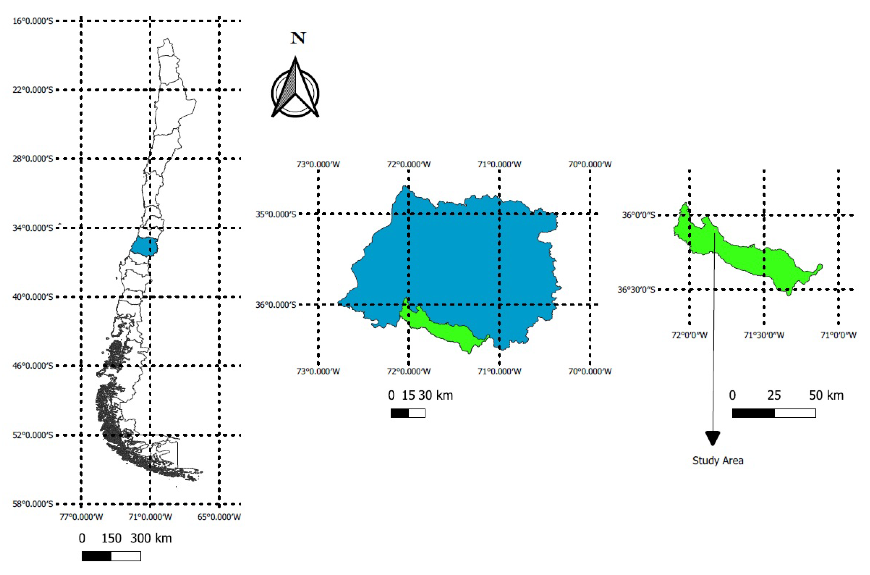
2.1. Field Trials
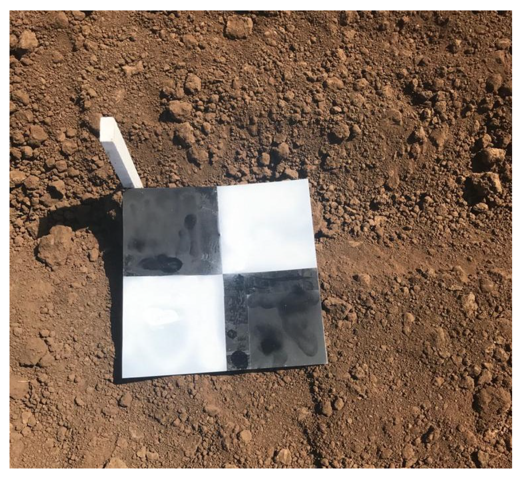
2.2. Images Acquisition from UAV
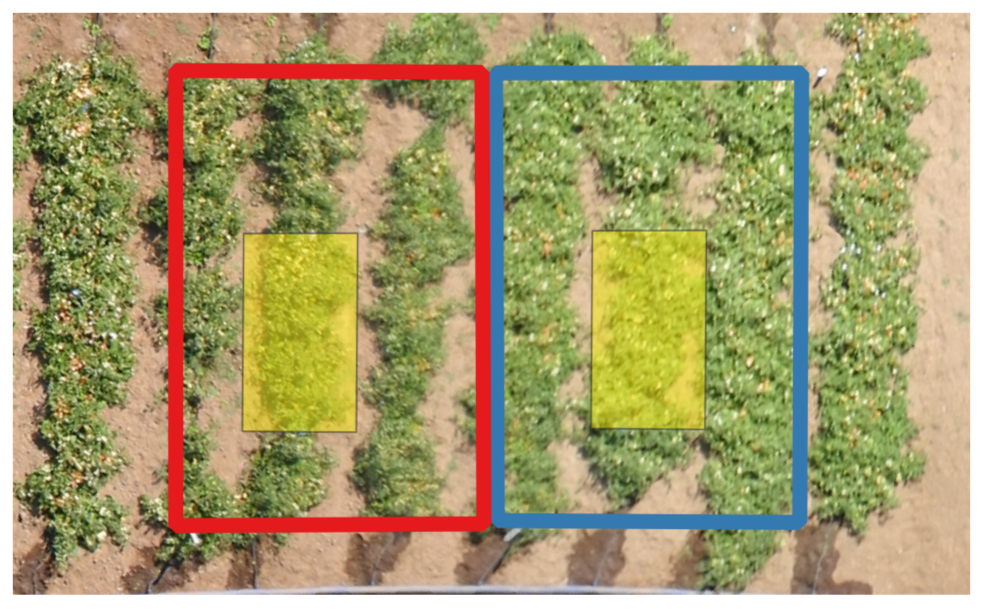
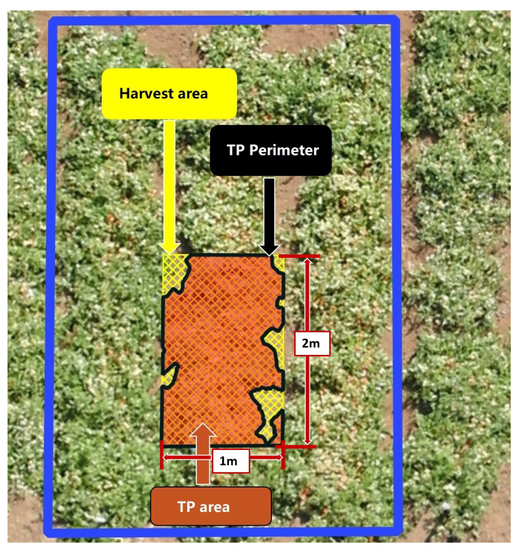
2.3. Agronomic Measurements
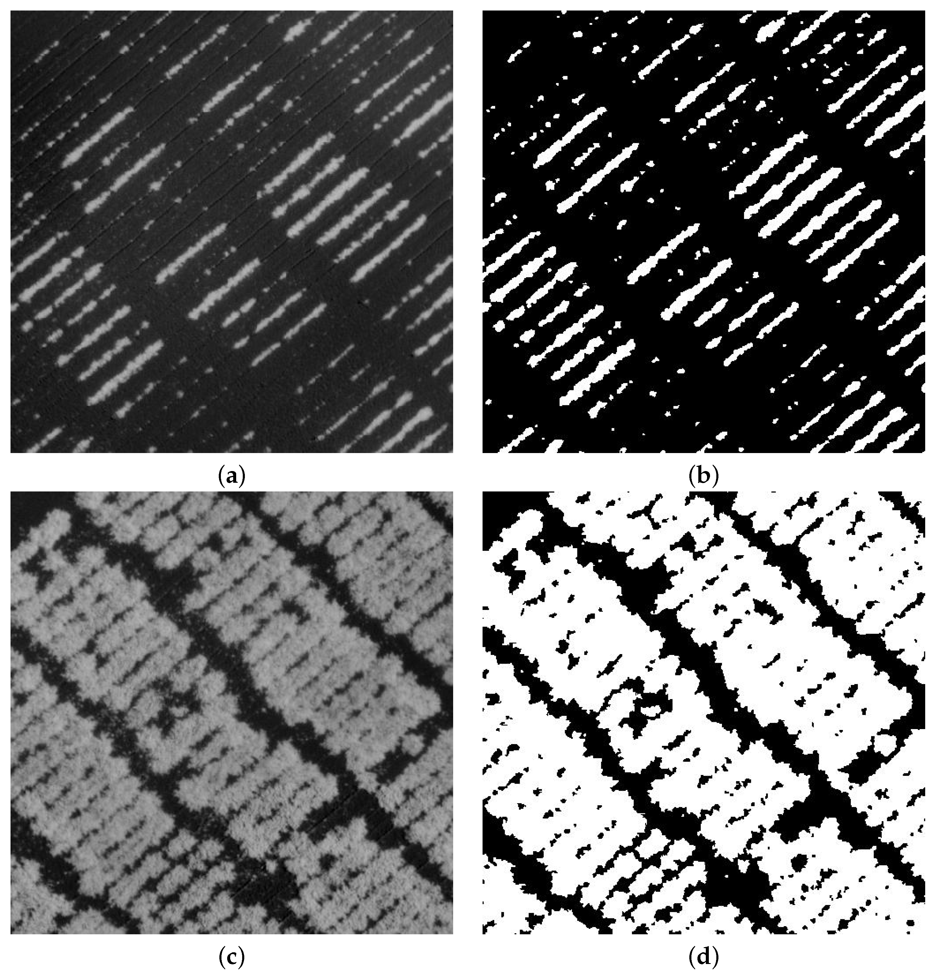
2.4. Images Segmentation
2.5. Data Sets
2.6. Forecasting Models for Processing Tomato Yield
3. Results and Discussion
4. Conclusions
Author Contributions
Funding
Conflicts of Interest
Sample Availability
References
- FAOSTAT. Foundation and Agricultural Organization of the Unites State. 2022. Available online: https://www.fao.org/faostat/en/#data/QI (accessed on 2 August 2022).
- The World Processing Tomato Council. WPTC: 2021 Crop Estimated at 38.7 Million Tonnes. 2021. Available online: https://www.tomatonews.com/en/wptc-2021-crop-estimated-at-387-million-tonnes_2_1489.html (accessed on 2 August 2022).
- Ashapure, A.; Oh, S.; Marconi, T.G.; Chang, A.; Jung, J.; Landivar, J.; Enciso, J. Unmanned aerial system based tomato yield estimation using machine learning. In Proceedings of the Autonomous Air and Ground Sensing Systems for Agricultural Optimization and Phenotyping IV, Baltimore, MD, USA, 15–16 April 2019; Volume 11008, p. 110080. [Google Scholar]
- Johansen, K.; Morton, M.J.L.; Malbeteau, Y.M.; Aragon, B.; Al-Mashharawi, S.K.; Ziliani, M.G.; Angel, Y.; Fiene, G.M.; Negrão, S.S.C.; Mousa, M.A.A.; et al. Unmanned Aerial Vehicle-Based Phenotyping Using Morphometric and Spectral Analysis Can Quantify Responses of Wild Tomato Plants to Salinity Stress. Front. Plant Sci. 2019, 10, 370. [Google Scholar] [CrossRef] [PubMed]
- Jongeneel, R.; Gonzalez-Martinez, A.R. Estimating crop yield supply responses to be used for market outlook models: Application to major developed and developing countries. NJAS-Wagening. J. Life Sci. 2020, 92, 100327. [Google Scholar] [CrossRef]
- Robson, A.; Rahman, M.M.; Muir, J. Using worldview satellite imagery to map yield in avocado (Persea americana): A case study in Bundaberg, Australia. Remote. Sens. 2017, 9, 1223. [Google Scholar] [CrossRef] [Green Version]
- Gao, F.; Zhang, X. Mapping crop phenology in near real-time using satellite remote sensing: Challenges and opportunities. J. Remote. Sens. 2021, 2021, 8379391. [Google Scholar] [CrossRef]
- Wei, M.C.F.; Maldaner, L.F.; Ottoni, P.M.N.; Molin, J.P. Carrot yield mapping: A precision agriculture approach based on machine learning. AI 2020, 1, 229–241. [Google Scholar] [CrossRef]
- Cuaran, J.; Leon, J. Crop monitoring using unmanned aerial vehicles: A review. Agric. Rev. 2021, 42, 121–132. [Google Scholar] [CrossRef]
- Velusamy, P.; Rajendran, S.; Mahendran, R.K.; Naseer, S.; Shafiq, M.; Choi, J.G. Unmanned Aerial Vehicles (UAV) in precision agriculture: Applications and challenges. Energies 2021, 15, 217. [Google Scholar] [CrossRef]
- Deng, L.; Mao, Z.; Li, X.; Hu, Z.; Duan, F.; Yan, Y. UAV-based multispectral remote sensing for precision agriculture: A comparison between different cameras. ISPRS J. Photogramm. Remote. Sens. 2018, 146, 124–136. [Google Scholar] [CrossRef]
- Yang, Q.; Shi, L.; Han, J.; Chen, Z.; Yu, J. A VI-based phenology adaptation approach for rice crop monitoring using UAV multispectral images. Field Crop. Res. 2022, 277, 108419. [Google Scholar] [CrossRef]
- Enciso, J.; Avila, C.A.; Jung, J.; Elsayed-Farag, S.; Chang, A.; Yeom, J.; Landivar, J.; Maeda, M.; Chavez, J.C. Validation of agronomic UAV and field measurements for tomato varieties. Comput. Electron. Agric. 2019, 158, 278–283. [Google Scholar] [CrossRef]
- Kwak, G.H.; Park, N.W. Impact of Texture Information on Crop Classification with Machine Learning and UAV Images. Appl. Sci. 2019, 9, 643. [Google Scholar] [CrossRef] [Green Version]
- Singhal, G.; Bansod, B.; Mathew, L.; Goswami, J.; Choudhury, B.; Raju, P. Chlorophyll estimation using multi-spectral unmanned aerial system based on machine learning techniques. Remote. Sens. Appl. Soc. Environ. 2019, 15, 100235. [Google Scholar] [CrossRef]
- Rakesh, D.; Kumar, N.A.; Sivaguru, M.; Keerthivaasan, K.; Janaki, B.R.; Raffik, R. Role of UAVs in Innovating Agriculture with Future Applications: A Review. In Proceedings of the 2021 International Conference on Advancements in Electrical, Electronics, Communication, Computing and Automation (ICAECA), Coimbatore, India, 8–9 October 2021; pp. 1–6. [Google Scholar]
- Hassan, M.A.; Yang, M.; Rasheed, A.; Yang, G.; Reynolds, M.; Xia, X.; Xiao, Y.; He, Z. A rapid monitoring of NDVI across the wheat growth cycle for grain yield prediction using a multi-spectral UAV platform. Plant Sci. 2019, 282, 95–103. [Google Scholar] [CrossRef] [PubMed]
- Senthilnath, J.; Dokania, A.; Kandukuri, M.; Ramesh, K.N.; Anand, G.; Omkar, S.N. Detection of tomatoes using spectral-spatial methods in remotely sensed RGB images captured by UAV. Biosyst. Eng. 2016, 146, 16–32. [Google Scholar] [CrossRef]
- Johansen, K.; Morton, M.J.; Malbeteau, Y.; Aragon, B.; Al-Mashharawi, S.; Ziliani, M.G.; Angel, Y.; Fiene, G.; Negrao, S.; Mousa, M.A.; et al. Predicting Biomass and Yield in a Tomato Phenotyping Experiment Using UAV Imagery and Random Forest. Front. Artif. Intell. 2020, 3, 28. [Google Scholar] [CrossRef]
- Johansen, K.; Morton, M.J.L.; Malbeteau, Y.; Aragon, B.; Al-Mashharawi, S.; Ziliani, M.; Angel, Y.; Fiene, G.; Negrao, S.; Mousa, M.A.A.; et al. Predicting biomass and yield at harvest of salt-stressed tomato plants using UAV imagery. ISPRS—Int. Arch. Photogramm. Remote. Sens. Spat. Inf. Sci. 2019, XLII-2/W13, 407–411. [Google Scholar] [CrossRef] [Green Version]
- Tatsumi, K.; Igarashi, N.; Mengxue, X. Prediction of plant-level tomato biomass and yield using machine learning with unmanned aerial vehicle imagery. Plant Methods 2021, 17, 1–17. [Google Scholar] [CrossRef]
- Gil-Docampo, M.L.; Arza-García, M.; Ortiz-Sanz, J.; Martínez-Rodríguez, S.; Marcos-Robles, J.L.; Sánchez-Sastre, L.F. Above-ground biomass estimation of arable crops using UAV-based SfM photogrammetry. Geocarto Int. 2020, 35, 687–699. [Google Scholar] [CrossRef]
- Sagi, O.; Rokach, L. Ensemble learning: A survey. WIREs Data Min. Knowl. Discov. 2018, 8, e1249. [Google Scholar] [CrossRef]
- Rodríguez, R.; Sossa, J.H. Procesamiento y Análisis Digital de Imágenes; Alfaomega Grupo Editor: Ciudad de México, México, 2012; ISBN 10:6077072230. [Google Scholar]
- Santibáñez, F. Atlas agroclimático de Chile. Estado Actual y Tendencias del Clima. Tomo III Regiones de Valparaíso, Metropolitana, del Libertador Bernardo O’Higgins y del Maule; Universidad de Chile, Facultad de Ciencias Agronómicas: Santiago, Chile, 2017. [Google Scholar]
- SensFly. Parrot Sequoia+ Cámara Multiespectral. 2020. Available online: https://www.sensefly.com/es/camera/parrot-sequoia (accessed on 21 March 2021).
- Pix4D. Pix4D Radiometric Calibration Target. 2020. Available online: https://support.pix4d.com/hc/en-us/articles/206494883-Radiometric-calibration-target (accessed on 21 March 2021).
- Grados, D.; Schrevens, E. Cassava NDVI Analysis: A Nonlinear Mixed Model Approach Based on UAV-Imagery. PFG—J. Photogramm. Remote. Sens. Geoinf. Sci. 2020, 88, 337–347. [Google Scholar] [CrossRef]
- Achanta, R.; Shaji, A.; Smith, K.; Lucchi, A.; Fua, P.; Süsstrunk, S. SLIC Superpixels Compared to State-of-the-Art Superpixel Methods. IEEE Trans. Pattern Anal. Mach. Intell. 2012, 34, 2274–2282. [Google Scholar] [CrossRef] [Green Version]
- Otsu, N. A Threshold Selection Method from Gray-Level Histograms. IEEE Trans. Syst. Man. Cybern. 1979, 9, 62–66. [Google Scholar] [CrossRef] [Green Version]
- Chen, Y.; Chen, D.; Yang, L.; Chen, L. Otsu’s thresholding method based on gray level-gradient two-dimensional histogram. In Proceedings of the 2010 2nd International Asia Conference on Informatics in Control, Automation and Robotics (CAR 2010), Wuhan, China, 6–7 March 2010; Volume 3, pp. 282–285. [Google Scholar] [CrossRef]
- Innani, S.; Dutande, P.; Baheti, B.; Talbar, S.; Baid, U. Fuse-PN: A Novel Architecture for Anomaly Pattern Segmentation in Aerial Agricultural Images. In Proceedings of the IEEE/CVF Conference on Computer Vision and Pattern Recognition, Nashville, TN, USA, 20–25 June 2021; pp. 2960–2968. [Google Scholar]
- Ramos, A.P.M.; Osco, L.P.; Furuya, D.E.G.; Gonçalves, W.N.; Santana, D.C.; Teodoro, L.P.R.; da Silva Junior, C.A.; Capristo-Silva, G.F.; Li, J.; Baio, F.H.R.; et al. A random forest ranking approach to predict yield in maize with uav-based vegetation spectral indices. Comput. Electron. Agric. 2020, 178, 105791. [Google Scholar] [CrossRef]
- Barnes, E.; Clarke, T.; Richards, S.; Colaizzi, P.; Haberland, J.; Kostrzewski, M.; Waller, P.; Choi, C.; Riley, E.; Thompson, T.; et al. Coincident detection of crop water stress, nitrogen status and canopy density using ground based multispectral data. In Proceedings of the Fifth International Conference on Precision Agriculture, Bloomington, MN, USA, 16–19 July 2000; Volume 1619, p. 6. [Google Scholar]
- Jorge, J.; Vallbé, M.; Soler, J.A. Detection of irrigation inhomogeneities in an olive grove using the NDRE vegetation index obtained from UAV images. Eur. J. Remote. Sens. 2019, 52, 169–177. [Google Scholar] [CrossRef] [Green Version]
- Ohashi, Y.; Murai, M.; Ishigami, Y.; Goto, E. Light-Intercepting Characteristics and Growth of Tomatoes Cultivated in a Greenhouse Using a Movable Bench System. Horticulturae 2022, 8, 60. [Google Scholar] [CrossRef]
- Breiman, L. Random forests. Mach. Learn. 2001, 45, 5–32. [Google Scholar] [CrossRef] [Green Version]
- Everingham, Y.; Sexton, J.; Skocaj, D.; Inman-Bamber, G. Accurate prediction of sugarcane yield using a random forest algorithm. Agron. Sustain. Dev. 2016, 36, 27. [Google Scholar] [CrossRef] [Green Version]
- Fukuda, S.; Spreer, W.; Yasunaga, E.; Yuge, K.; Sardsud, V.; Müller, J. Random Forests modelling for the estimation of mango (Mangifera indica L. cv. Chok Anan) fruit yields under different irrigation regimes. Agric. Water Manag. 2013, 116, 142–150. [Google Scholar] [CrossRef]
- Patrignani, A.; Ochsner, T.E. Canopeo: A Powerful New Tool for Measuring Fractional Green Canopy Cover. Agron. J. 2015, 107, 2312–2320. [Google Scholar] [CrossRef]


| Parameter | Ebee SQ |
|---|---|
| Camera | Parrot Sequoia |
| Flight Height | |
| Lateral Overlap | 80% |
| Vertical Overlap | 80% |
| Number of Images Per Flight | 41 per band |
| Spatial Resolution |
| Flight | Date | Day after Transplant | Weeks before Harvest (WBH) |
|---|---|---|---|
| 1 | 21 November, 2019 | 44 | 12 |
| 2 | 30 November 2019 | 53 | 11 |
| 3 | 11 December 2019 | 64 | 10 |
| 4 | 11 January 2020 | 95 | 5 |
| 5 | 25 January 2020 | 109 | 3 |
| 6 | 29 January 2020 | 113 | 3 |
| 7 | 5 February 2020 | 120 | 2 |
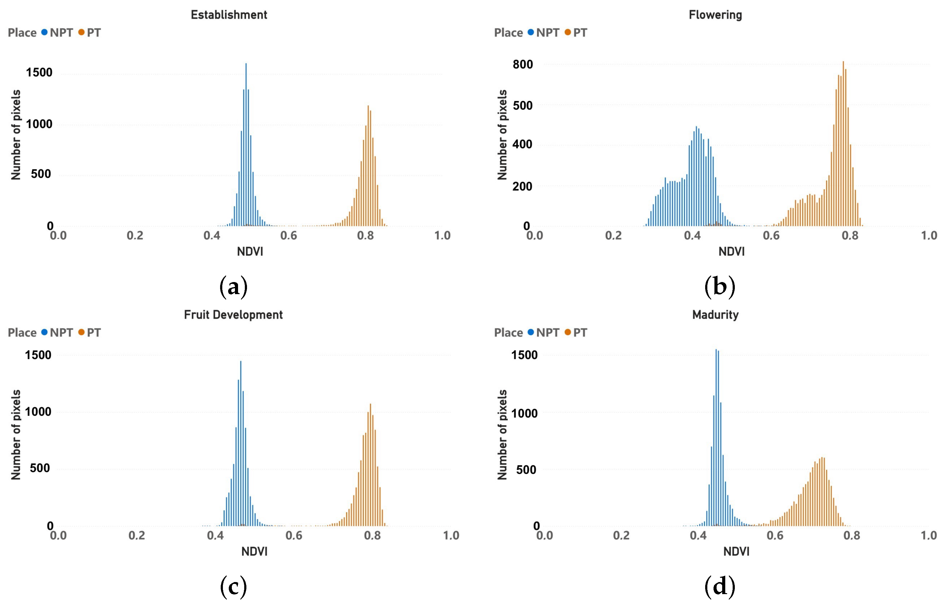
| Date | Phenological Stage | Dice |
|---|---|---|
| 21 November 2019 | Establishment | 0.896 |
| 30 November 2019 | Vegetative Growth | 0.938 |
| 11 December 2019 | Flowering | 0.947 |
| 11 January 2020 | Fruit Development | 0.976 |
| 25 January 2020 | Fruit Development | 0.978 |
| 29 January 2020 | Maturity | 0.979 |
| 05 February 2020 | Maturity | 0.971 |
| 20 February 2020 | Maturity | 0.957 |
| Accumulated Characteristics | Specific Characteristics | |||
|---|---|---|---|---|
| DTE-Bag | DTE-Boost | DTE-Bag | DTE-Boost | |
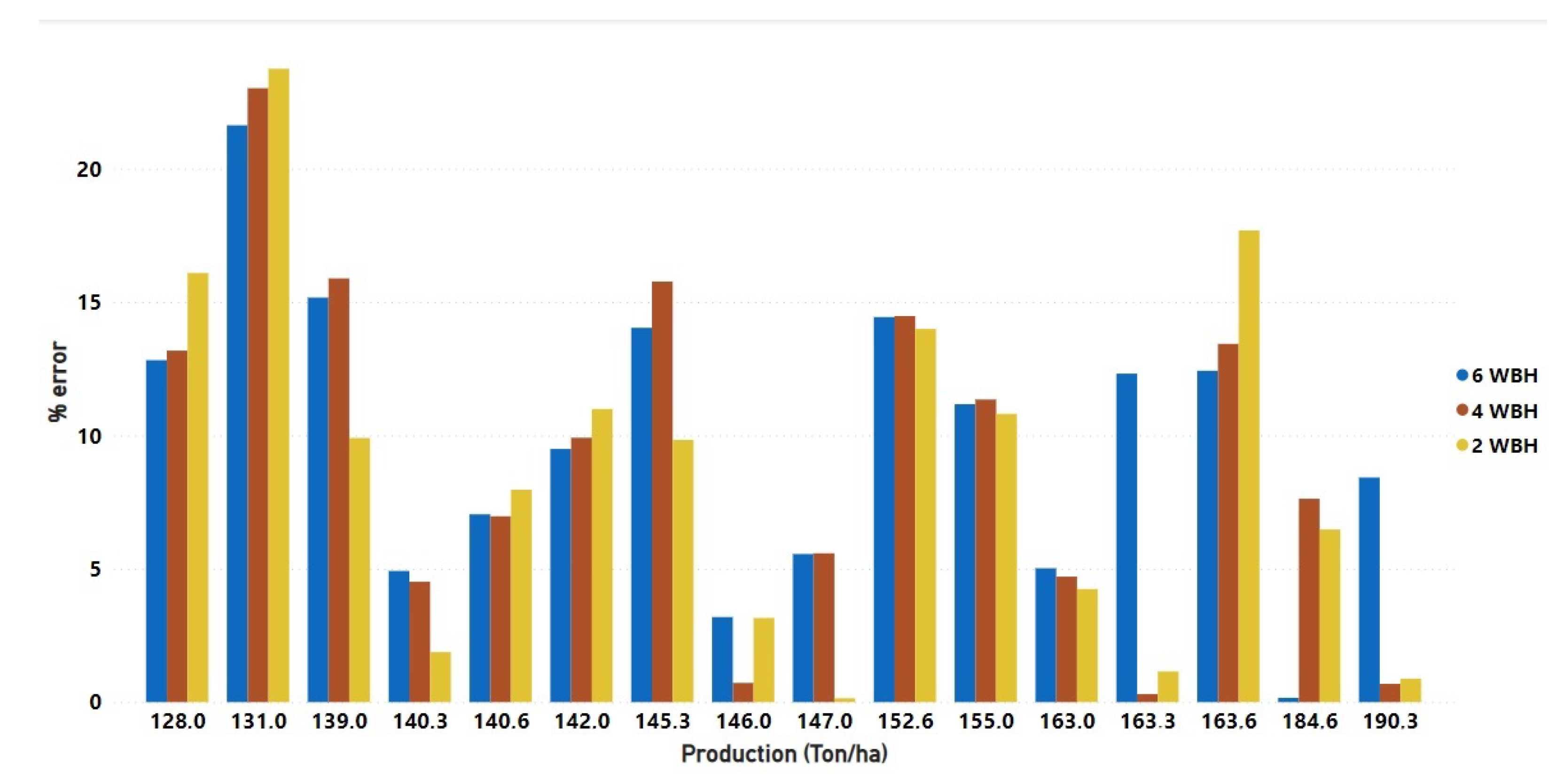
| 6 WBH | ||||
| RMSE (Ton/ha) | 14.38 | 16.65 | 14.07 | 13.34 |
| Percentage error | 9.28% | 10.82% | 8.86 % | 8.5 % |
| Standard deviation (Ton/ha) | 9.86 | 10.61 | 11.17 | 8.57 |
| RMSE maximum (Ton/ha) | 41.16 | 40.09 | 42.29 | 30.43 |
| 4 WBH | ||||
| RMSE (Ton/ha) | 13.65 | 13.22 | 15.67 | 16.13 |
| Percentage Error | 8.81% | 8.58% | 10.14% | 10.26% |
| Standard deviation (Ton/ha) | 11.09 | 10.67 | 8.25 | 13.20 |
| RMSE maximum (Ton/ha) | 43.81 | 36.88 | 29.28 | 41.52 |
| 2 WBH | ||||
| RMSE (Ton/ha) | 12.87 | 14.47 | 14.30 | 17.05 |
| Percentage error | 8.17% | 9.14% | 9.26% | 11.33% |
| Standard deviation (Ton/ha) | 11.11 | 13.13 | 10.80 | 13.09 |
| RMSE Maximum (Ton/ha) | 45.20 | 53.75 | 41.91 | 38.72 |
| Low Range Production | High Range Production | |||||
|---|---|---|---|---|---|---|
| Attribute | 6 WBH | 4 WBH | 2 WBH | 6 WBH | 4 WBH | 2 WBH |
| NDVI’ | 0.56 | 0.59 | 0.60 | 0.71 | 0.72 | 0.70 |
| NDRE’ | 0.51 | 0.55 | 0.60 | 0.68 | 0.70 | 0.74 |
| FFC’ | 0.36 | 0.52 | 0.83 | 0.42 | 0.59 | 0.91 |
| FFS’ | 0.34 | 0.48 | 0.76 | 0.40 | 0.57 | 0.86 |
| FFD’ | 0.47 | 0.57 | 0.80 | 0.39 | 0.47 | 0.68 |
Publisher’s Note: MDPI stays neutral with regard to jurisdictional claims in published maps and institutional affiliations. |
© 2022 by the authors. Licensee MDPI, Basel, Switzerland. This article is an open access article distributed under the terms and conditions of the Creative Commons Attribution (CC BY) license (https://creativecommons.org/licenses/by/4.0/).
Share and Cite
Lillo-Saavedra, M.; Espinoza-Salgado, A.; García-Pedrero, A.; Souto, C.; Holzapfel, E.; Gonzalo-Martín, C.; Somos-Valenzuela, M.; Rivera, D. Early Estimation of Tomato Yield by Decision Tree Ensembles. Agriculture 2022, 12, 1655. https://doi.org/10.3390/agriculture12101655
Lillo-Saavedra M, Espinoza-Salgado A, García-Pedrero A, Souto C, Holzapfel E, Gonzalo-Martín C, Somos-Valenzuela M, Rivera D. Early Estimation of Tomato Yield by Decision Tree Ensembles. Agriculture. 2022; 12(10):1655. https://doi.org/10.3390/agriculture12101655
Chicago/Turabian StyleLillo-Saavedra, Mario, Alberto Espinoza-Salgado, Angel García-Pedrero, Camilo Souto, Eduardo Holzapfel, Consuelo Gonzalo-Martín, Marcelo Somos-Valenzuela, and Diego Rivera. 2022. "Early Estimation of Tomato Yield by Decision Tree Ensembles" Agriculture 12, no. 10: 1655. https://doi.org/10.3390/agriculture12101655