RSMDA: Random Slices Mixing Data Augmentation

Abstract

Advanced data augmentation techniques have demonstrated great success in deep learning algorithms. Among these techniques, single-image-based data augmentation (SIBDA), in which a single image’s regions are randomly erased in different ways, has shown promising results. However, randomly erasing image regions in SIBDA can cause a loss of the key discriminating features, consequently misleading neural networks and lowering their performance. To alleviate this issue, in this paper, we propose the random slices mixing data augmentation (RSMDA) technique, in which slices of one image are placed onto another image to create a third image that enriches the diversity of the data. RSMDA also mixes the labels of the original images to create an augmented label for the new image to exploit label smoothing. Furthermore, we propose and investigate three strategies for RSMDA: (i) the vertical slices mixing strategy, (ii) the horizontal slices mixing strategy, and (iii) a random mix of both strategies. Of these strategies, the horizontal slice mixing strategy shows the best performance. To validate the proposed technique, we perform several experiments using different neural networks across four datasets: fashion-MNIST, CIFAR10, CIFAR100, and STL10. The experimental results of the image classification with RSMDA showed better accuracy and robustness than the state-of-the-art (SOTA) single-image-based and multi-image-based methods. Finally, class activation maps are employed to visualize the focus of the neural network and compare maps using the SOTA data augmentation methods.

1. Introduction

Deep learning (DL) has shown a significant performance gain in various domains, including image classification [1,2,3,4,5,6,7,8,9,10], audio classification [11,12,13,14,15,16,17], and text classification [18,19,20]. This performance gain is due to three major factors [21]: (i) deep neural network architectures’ progress, (ii) high computational power, and (iii) access to large-scale data [21]. Among these factors, research on data has been the hot topic considering that DL convolutional neural networks (CNNs) require a huge amount of data. The data is required for better generalization, which, in turn, can prevent and reduce overfitting. Overfitting occurs when the network performance on training data becomes very high, and the network performance on unseen (validation) data worsens; alternatively, overfitting can be observed when the training error is low but the unseen (validation) error is high. There are two major categories of approaches to prevent overfitting. The first is model regularization [22], which is a technique that selects the desired model’s complexity level, or the level at which the model provides better generalization. Examples of this class are batch normalization [23] and dropout [24]. The second category is data augmentation [21,25,26,27], which uses or re-mixes existing data to create new and more diverse training data. There are different data augmentations (DAs), divided into two categories; (i) traditional data augmentations such as flipping [21,25], cropping [21,25], resizing [25], and many more [21] and (ii) advanced data augmentation. Recent research has demonstrated that traditional data augmentations do not provide enough diversity for the highly parameterized CNN architectures, and, as a result, they can overfit easily [27,28,29,30,31]. Thus, advanced data augmentations have ignited the interest of the research community. Examples of advanced data augmentations are random erasing (RE) [25], hide and seek (HS) [32], GridMask [33], CutOut [34], MixUp [35], CutMix [36], RICAP [27], mixed example data augmentations [37], and many more [21]. Single-image deletion has been studied by many researchers with techniques such as RE, HS, GridMask, and CutOut. Furthermore, multi-image mixing techniques have been studied, such as CutMix, MixUp, RICAP, and many others [21]. Single-image deletion and multi-image mixing techniques are illustrated in Figure 1. Single-image deletion techniques may lose features, consequently deteriorating the performance of DL models, and multi-image mixing techniques have explored augmentations from different perspectives, but none have considered data augmentation based on slice mixing. To the best of our knowledge, we are the first to explore random slices mixing to check the effect of the proposed data augmentation technique using different strategies, namely, the horizontal (row-wise) slices mixing strategy, the vertical (column-wise) slices mixing strategy, and a mixture of both, as shown in Figure 2. The research question we address is: can the proposed data augmentation technique preserve the features’ information lost in single-image data augmentations? The proposed technique obtains slices of one image and places them onto another image to create a third image and enrich the variety of training images available. In our previous work [38], we introduced only horizontal slice mixing and validated the approach for the limited models without finding the optimal hyperparameters, such as the probability and slice size. In this work, we are extending the previous work [38] to vertical slice mixing and a mixture of both, and are using numerous bigger models in addition to finding the optimal hyperparameters. Furthermore, robustness against adversarial attacks is checked, and RSMDA class activation maps are compared with other SOTA methods to visualize the focus of the models. In the remainder of the paper, the terms “network” and “model” are used interchangeably.

The rest of the paper is organized as follows: Section 2 describes the literature review; Section 3 explains the proposed method; Section 4 provides the experimental details, results, adversarial attacks, and class activation maps; and, finally, Section 5 concludes the work.

2. Related Work

The main purpose of using data augmentation is to prevent a model from overfitting. RSMDA is broadly related to regularization as data augmentation is itself an explicit form of regularization [25,26,39,40]. We consider related works that fall into two main categories: (i) dropout as a regularization technique and (ii) data augmentation. These will be discussed in what follows.

2.1. Dropout

A lot of research has been completed on dropout [24,41,42,43,44]. Dropout [24,41], introduced by Hinton et al., is a regularization technique, in which hidden and visible neural network neurons are randomly set to zero with some probability and are dropped during training. The advantage of this technique is that it averages several smaller sub-networks to not only boost the generalization capability but also to improve the robustness against adversarial attacks. With the passage of time, it was noticed that dropout regularization works well with densely or fully connected layers, but it does not perform well with convolutional layers (CLs) [45]. There are two main reasons for this not working well with CLs: (i) CLs have far fewer parameters than densely connected layers and need much less regularization. (ii) On the image level, if we drop out the pixel in the image, the remaining neighboring pixels will provide enough information; therefore, performing regularization does not have the same effect as it has on the model level in the case of fully connected layers. Later on, many variants of dropouts have been proposed to improve the effectiveness of a simple dropout. In [42], an adaptive dropout is proposed as an extension of dropout, where the probability of a hidden neuron being discarded is calculated using a binary belief network. Technically, there are different probabilities for different neurons. DropConnect [43] is another extension of dropout that randomly selects the subsets of weights and sets them to zero instead of setting the subset of the activation to zero. SpatialDropout [45] is another extension of dropout that randomly ignores whole feature maps instead of individual pixels, which helps cater to the problem of neighboring pixels passing on redundant information. In stochastic pooling [44], parameter-free activations are selected during training from a multinomial distribution and used with SOTA regularization techniques. Stochastic pooling can be combined with data augmentation or dropout.

2.2. Data Augmentation

Data augmentation is another regularization technique. Technically, data augmentation enlarges the number of training samples using existing training dataset samples; therefore, it increases the performance of deep learning models. Most data augmentation techniques create different flavors of existing samples during training, thereby providing many different views of such samples to increase the diversity of data. Recently, there has been a lot of work performed on data augmentation [21,25,27,32,33,34,37]. For a clearer understanding of the different aspects involved, we divide the related data augmentation approaches into two categories: (i) single-image-based data augmentation and (ii) multi-image-based data augmentation. Each of them is discussed separately in the remainder of this section.

2.2.1. Single-Image-Based Data Augmentation (SIBDA)

Single-image-based data augmentation refers to the data augmentation approaches in which only a single image is required for augmentation. This is the case for traditional augmentation approaches, such as flipping, rotating, etc. These days, SIBDA techniques have advanced from occlusion perspectives, such as random erasing, CutOut, and many more [21]. Closely related SIBDAs are discussed below.

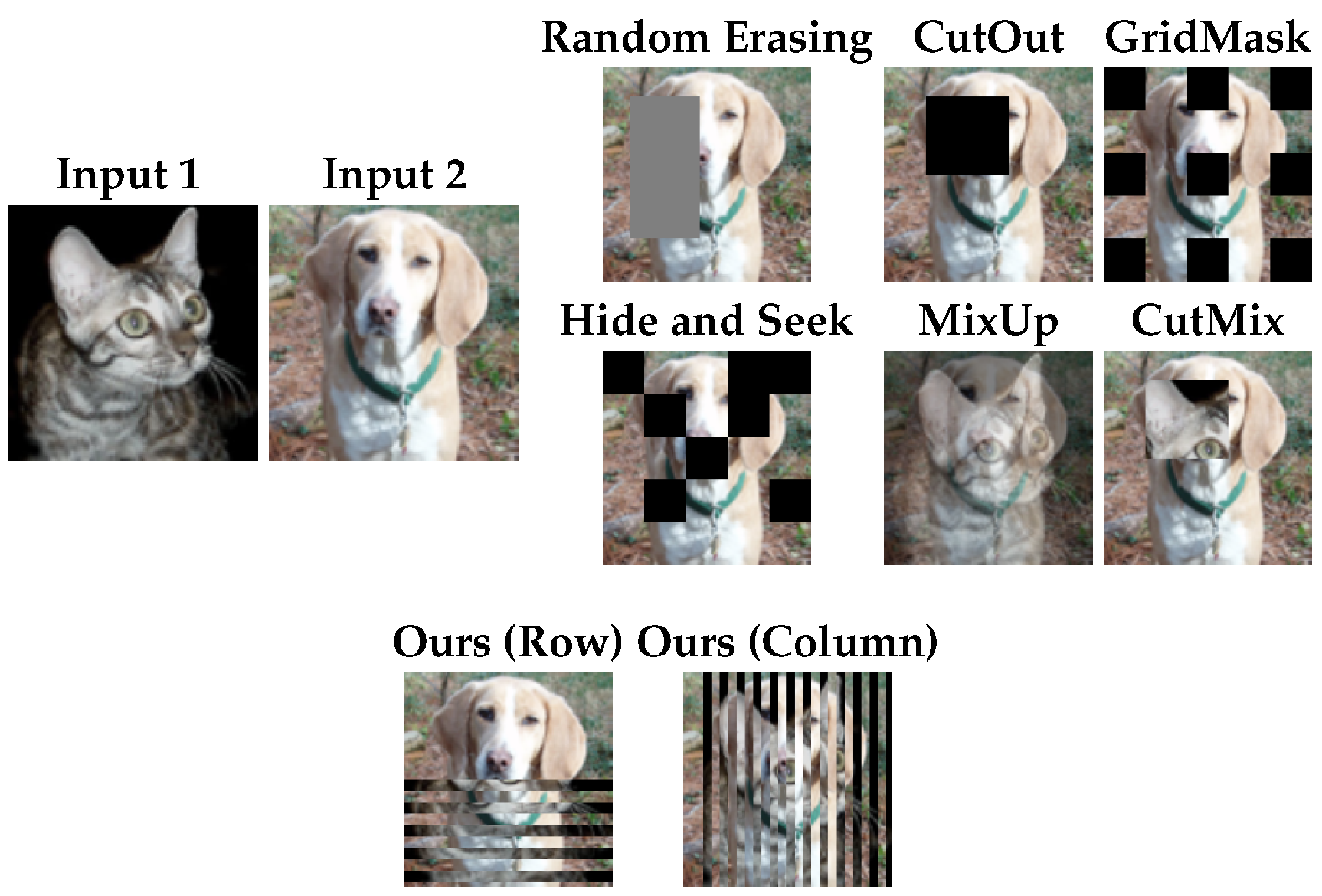
• CutOut: CutOut [34] is data augmentation in which a random part of the image is cut with a square and filled with 0, 255, or the mean of the dataset during training. It was introduced with the purpose of recognizing partially or fully occluded object(s).
• Random erasing: Random erasing (RE) [25] is a data augmentation technique in which a rectangular random region of the image is selected at random and erased with a random value with the aim of minimizing overfitting. During training, different occlusion levels are performed not only to improve the performance of the neural network but also to improve the robustness of the model. RE was designed to deal with occlusion in images, thereby forcing the model to learn the erased features. Here, occlusion is where some part(s) of the image is not clear. RE seems similar to CutOut, but the key difference is that RE randomly determines whether to mask out or not, and it determines the aspect ratio and size of the masked region. On the other hand, CutOut does not consider the aspect ratio.
• Hide and Seek: Hide and seek (HS) [32] is another data augmentation technique in which the image is divided into squares of the same size as a grid. During the training at each step, a random number of squares is hidden to force the neural network to focus on the most discriminated parts and learn the relevant features. At each epoch, it gives a different view of the image being modeled to learn the important features.
• GridMask: GridMask [33] is a type of data augmentation in which uniform masking is applied to mask out regions in the image and the mask square size changes at each step. Previously discussed data augmentations, such as a CutOut, RE, and HS, randomly erase the region(s) in which there are high chances that either an object is removed or contextual information is lost, which can potentially harm the performance of the model. To trade off between losing contextual information or object removal and performance, GridMask is introduced.

All of the above SIBDAs have higher chances of losing useful features and, at the same time, are not taking advantage of label smoothing. Label smoothing refers to whatever portion or percentage of the image is erased or mixed; corresponding labels should be mixed in the same ratio. To cater to these features or to information loss, we propose a novel approach named random slices mixing data augmentation (RSMDA). The RSMDA approach is different from SIBDAs because, firstly, it requires two images, and, secondly, it enjoys the benefits of label smoothing. It is logically correct that, whatever portion of the images have mixed, the corresponding labels should be mixed accordingly, as performed in [27,35,36].

2.2.2. Multi-Image-Based Data Augmentation

Multi-image-based data augmentation (MIBDA) refers to the data augmentation category where it requires more than one image to create the augmented image. Several methods exist for MIBDA, such as MixUp [35], CutMix [36], RICAP [27], mixed example data augmentations [37], and many more [21]. We have limited the MIBDA techniques’ literature review so that is closely related to the proposed technique.

• MixUp: MixUp [35] is a data augmentation that creates a new augmented image using a weighted combination of two images, and label smoothing is performed simultaneously. It demonstrated impressive performance on a variety of tasks.
• CutMix: CutMix [36], a data augmentation method, is introduced to deal with the problems of information loss and the inefficiency of regional dropout methods. In CutMix, a random region of one image is replaced with a patch from another image, and the corresponding labels are mixed as well. It demonstrates high regularization in a wide range of tasks. This method uses only two images.
• Random Image Cropping and Patching Data Augmentation for Deep CNNs (RICAP): RICAP [27] is another data augmentation technique that is similar to CutMix except that it uses four images. RICAP further increases the diversity of the training data, enabling it to learn more features; it has shown good performance. More importantly, the labels of the four images are also mixed.
• Improved Mixed Example Data Augmentation: Improved mixed example data augmentation (IMEDA) [37] is another data augmentation that explores augmentation to check the importance of linearity using non-label preserving data augmentations in its search space. IMEDA explores the number of data augmentations and shows a massive performance gain over the SOTA methods.

All of the MIBDA techniques have explored data augmentation from different mixing points of view, which is closely relevant to RSMDA. The key difference between the previous works and RSMDA is that none of these previous data augmentations individually explored data augmentation from a slice mixing point of view. To the best of our knowledge, we are the first to explore data augmentation from a slice mixing point of view in detail. We make the following contributions to this work.

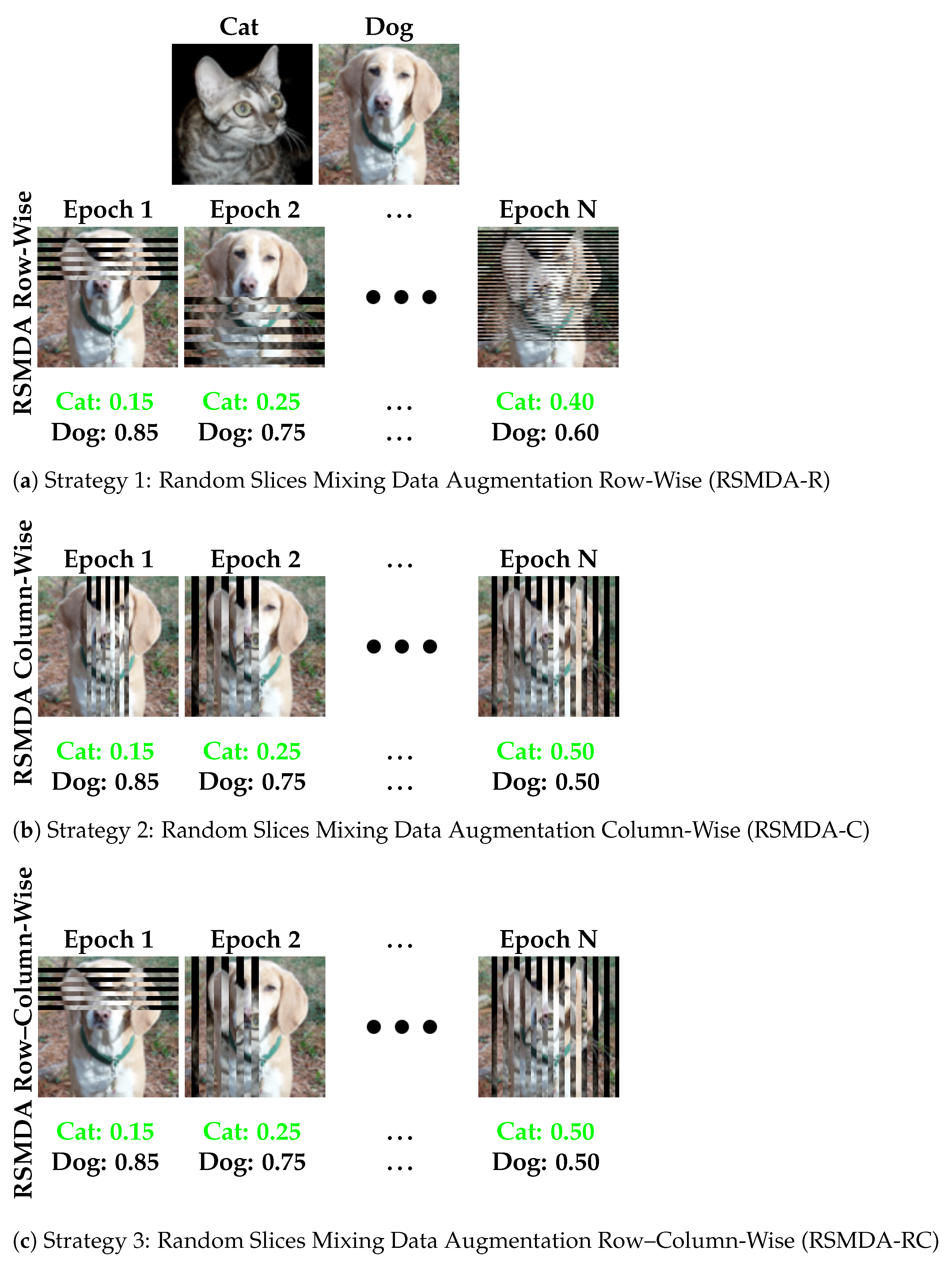
• We propose a novel data augmentation technique named random slices mixing data augmentation (RSMDA).
• We propose and investigate three different RSMDA strategies, namely, horizontal (row-wise) slice mixing, vertical (column-wise) slice mixing, and a combination of both.
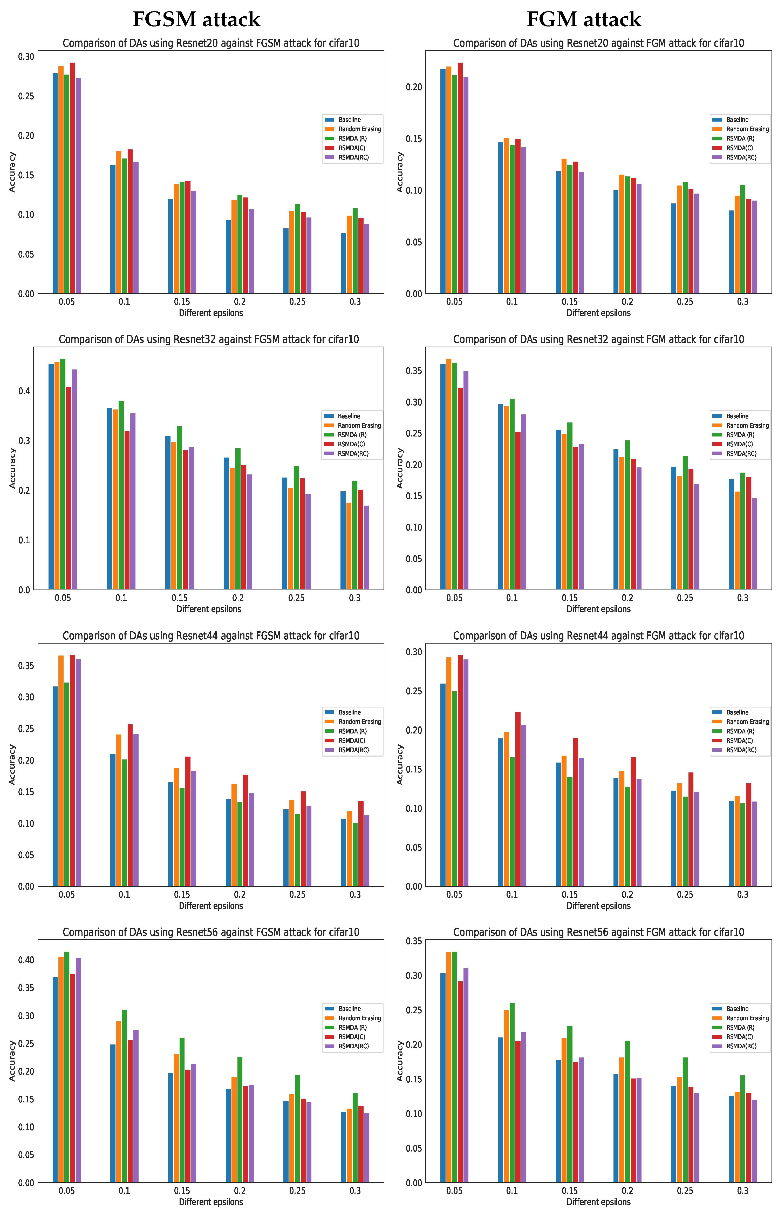
• We validate this approach using different models’ architectures across different datasets. RSMDA is not only effective in its accuracy performance but also robust against adversarial attacks.
• We investigate the RSMDA hyperparameters in detail, provide analysis, and compare them with SOTA augmentations using class activation maps (CAMs).
• Finally, we provide the full source code for RSMDA in an open repository: https://github.com/kmr2017/Slices-aug (accessed on 8 December 2022).

3. Proposed Method

Let $\mathit{x}\in {\mathbb{R}}^{W\times H\times C}$ and y represent a training image and its label, respectively. The main idea of RSMDA is to create a new training image with its label $(\tilde{\mathit{x}},\tilde{\mathit{y}})$. For that purpose, we select two training samples with corresponding labels, $({\mathit{x}}_1,{\mathit{y}}_1)$ and $({\mathit{x}}_2,{\mathit{y}}_2)$. A combination of these training samples can be defined as:

$$\tilde{\mathit{x}}=M\odot {\mathit{x}}_1+(1-M)\odot {\mathit{x}}_2$$

(1)

Additionally, their labels’ combination is defined as:

$$\tilde{\mathit{y}}=\lambda \odot {\mathit{y}}_1+(1-\lambda )\odot {\mathit{y}}_2$$

(2)

where $M\in {[0,1]}^{W\times H}$ is a binary mask that is filled with 0 and 1, where 0 and 1 are for excluding and including the image pixel, respectively. The symbol ⊙ shows element-wise multiplication, and $\lambda$ is the combination ratio of the two images and their labels, which is sampled from a beta distribution, such as CutMix [36] or MixUp [35]. In $Beta(\alpha ,\alpha )$, we set alpha to 1, following previous data augmentation, and $\lambda$ is distributed technically from the normal distribution.

For sampling the binary mask M, we randomly obtain slices of the size S in a certain range. To obtain the total number of slices, we divide W or H by S.

In the case of the total number of column slices:

$$TotalSlices=\lfloor W/S\rfloor$$

(3)

In the case of the total number of row slices:

$$TotalSlices=\lfloor H/S\rfloor$$

(4)

The next step is to ascertain how many slices should be mixed. To obtain this, we multiply the total slices by $\lambda$, which gives the number of slices to be mixed.

$$N_{mix}=\lfloor \lambda \times TotalSlices\rfloor$$

(5)

In Equation (5), $N_{mix}$ is the number of slices to be selected from the target sample and pasted to the source image. To do so, we fill $N_{mix}$ number of slices in mask M with 1 to select the slices from the target image. In order to generate an augmented sample pair $(\tilde{\mathit{x}},\tilde{\mathit{y}})$, the selected slices from the target image are pasted to a source image. Then, the $(\tilde{\mathit{x}},\tilde{\mathit{y}})$ augmented pair is used for training the model.

Furthermore, we propose and investigate the three different strategies of the proposed technique. Each of them is discussed below:

• Random slices mixing row-wise (RSMDA-R): In this strategy, we obtain $N_{mix}$ number of slices horizontally from the target image and paste it to the source image. Their corresponding labels are also mixed following the whole process discussed in Section 3. RSMDA-R is shown in Figure 2a.
• Random slices mixing column-wise (RSMDA-C): This is another strategy that we explore, in which we follow the same method used in RSMDA-R, except that we obtain the slices vertically, as shown in Figure 2b.
• Random slices mixing row–column-wise (RSMDA-RC): This is the third strategy. We apply both RSMDA-R and RSMDA-C based on binary randomness to each learning step, as shown in Figure 2c.

4. Experimental Results

In this section, we discuss the experimental setup, the dataset, and the results.

4.1. Experimental Setup

In our work, we used many network types, such as Resnet [40], VGG [26], and PyramidNet [46]. For a fair comparison with SIBDAs, we employed the same parameters as in [25]; this work [25] used 300 epochs, an initial learning rate of 0.1, continuous reduction by 10 at certain epochs (100, 150, 175, and 190), and a batch size set to 64. The probability of performing RSMDA was set to 0.5, similar to RE, and we also checked 10 different probabilities, as mentioned in Section 4.3.1. We re-performed the baseline and RE experiments for the fashionMNIST dataset as the original experiments [25] performed for the baseline and RE were on the old fashionMNIST dataset. The issue with the old fashionMNIST dataset is that a few test and training images overlapped with each other, as discussed in the GitHub repository (https://github.com/zhunzhong07/Random-Erasing/issues/9, accessed on 1 December 2022) of RE [25]. For a fair comparison with MIBDAs, we used the same setting as was mentioned in CutMix [36], where the epochs were 300, the batch size was 128, the initial learning rate was 0.1, the momentum was 0.9, and the learning rate decayed by 10 after every 30 epochs. We performed all of the experiments using a PyTorch module with 2 NVIDIA GetForce RTX 2080 Ti GPUs. Similar to the previous settings, each experiment was repeated at least three times unless otherwise mentioned.

4.2. Datasets

To validate the proposed approach, four different datasets were used. The datasets include color datasets of different sizes of images, such as CIFAR10 [47], CIFAR100 [47], and STL10 [48]. Then, a grayscale dataset, such as fashionMNIST [49] is used for the experiments.

4.2.1. FashionMNIST

The fashionMNIST dataset consists of 60,000 training and 10,000 test images. Each image is in grayscale and has the dimensions of 28 × 28, and there are 10 clothing classes in this dataset, namely, t-shirt/top, trouser, pullover, dress, coat, sandal, shirt, sneaker, bag, and ankle boot.

4.2.2. CIFAR10 and CIFAR100

Both the cifar10 and cifar100 datasets have an equal number of training and test images. Each dataset has 50,000 training and 10,000 test images, and each image is an RGB color image and has the dimensions of $32\times 32\times 3$. There are 10 and 100 classes in the cifar10 and cifar100 datasets, respectively.

4.2.3. STL10

We shifted the experiments to slightly greater dimensions, so we chose the STL10 dataset. It has only 500 training images and 8000 test images. Each image is in RGB color and of the dimensions $96\times 96\times 3$. There are 10 classes in this dataset. Images in this dataset are taken from one of the biggest datasets, ImageNet [39].

4.3. Results

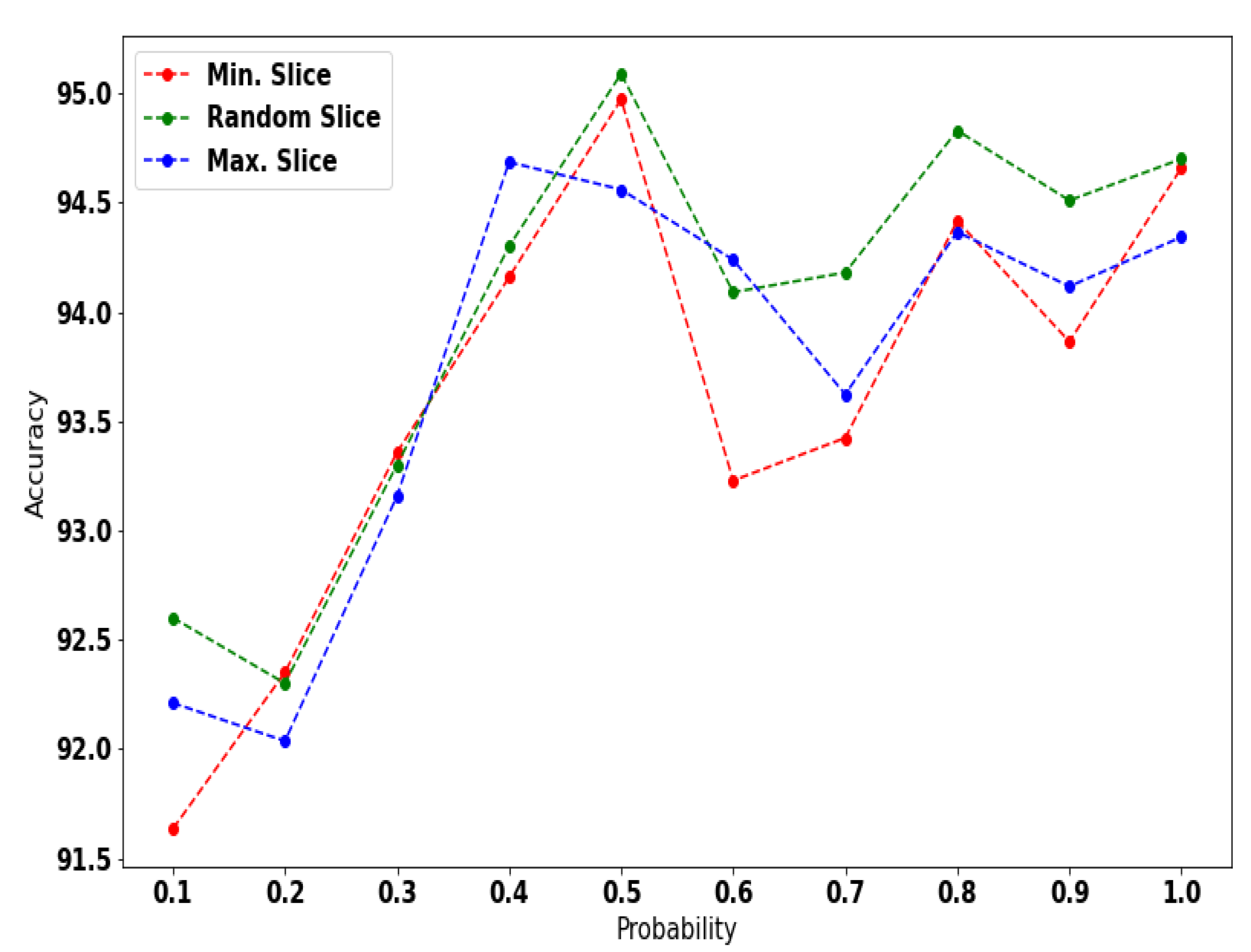
4.3.1. Hyperparameter Study

In our approach, we find the best probability of performing RSMDA and the best slice size using the ResNet20 model and the fashionMNIST dataset. In order to find the best probability, we performed experiments using different probabilities starting from 0.1 to 1.0 with 0.1 intervals, and it was found that 0.5 was the best probability. To find the optimal slice size, we investigate a slice size of two as the minimum, one-third of the image height or width as the maximum, and a random slice size between the minimum and maximum with each batch of images. The best parameters were found to be 0.5 for the best probability, and the random slice size was the best slice size, as shown in Figure 3, in which the x-axis, the three different color lines, and the y-axis show the probability of performing RSMDA, the slice size, and accuracy, respectively. For all of the remaining experiments, we used the best parameters.

Note, here, accuracy is defined as the percentage of correctly predicted samples, which is mathematically defined as:

$$A=100\ast C/T$$

(6)

where A, C, and T are the accuracy percentage, the number of correctly predicted samples, and the total number of samples, respectively. Therefore, higher accuracy is preferred. The error rate is the percentage of incorrectly predicted samples and can be defined as:

$$E=100-A$$

(7)

where E is the error rate, and A is the accuracy percentage. Therefore, a lower error rate is preferred.

We performed a number of experiments using different networks and datasets with three strategies. First, we compare our three strategies’ results with random erasing data augmentation and the baseline of different models, as shown in

Table 1. Performance comparison of the proposed approach with random erasing and baseline. First best and second best performances are highlighted in blue and red color, respectively.

Models	Baselines	RE	RSMDA (R)	RSMDA(C)	RSMDA(RC)
Fashion-MNIST
ResNet20	6.21 ± 0.11	5.04 ± 0.10	4.91 ± 0.12	4.72 ± 0.13	4.76 ± 0.06
Resnet32	6.04 ± 0.13	4.84 ± 0.12	4.81 ± 0.17	4.65 ± 0.15	4.81 ± 0.12
Resnet44	6.08 ± 0.16	4.87 ± 0.1	4.07 ± 0.14	4.784 ± 0.01	4.9 ± 0.25
Resnet56	6.78 ± 0.16	5.02 ± 0.11	5.00 ± 0.19	5.00 ± 0.2	5.09 ± 0.59
CIFAR10
Resnet20	7.21 ± 0.17	6.73 ± 0.09	7.18 ± 0.13	7.38 ±0.254	7.48 ± 1.08
Resnet32	6.41 ± 0.06	5.66 ± 0.10	6.31 ± 0.14	6.06 ± 0.101	6.21 ± 0.76
Resnet44	5.53 ± 0.0	5.13 ± 0.09	5.09 ± 0.10	5.26 ± 0.262	5.51 ± 0.06
Resnet56	5.31 ± 0.07	4.89 ± 0.0	5.02 ± 0.11	5.28 ± 0.02	5.97 ± 0.47
VGG11	7.88 ± 0.76	7.82 ± 0.65	7.80 ± 0.65	7.82 ± 0.27	7.81 ± 0.57
VGG13	6.33 ± 0.23	6.22 ± 0.63	6.18 ± 0.54	6.31 ± 0.266	6.20 ± 0.38
VGG16	6.42 ± 0.34	6.21 ± 0.76	6.20 ± 0.34	6.26 ± 0.196	6.35 ± 0.76
CIFAR100
Resnet20	30.84 ± 0.19	29.97 ± 0.11	30.18 ± 0.27	30.28 ± 0.33	30.46 ± 0.79
Resnet32	28.50 ± 0.37	27.18 ± 0.32	27.08 ± 0.34	28.22 ± 0.22	28.42 ± 0.12
Resnet44	25.27 ± 0.21	24.29 ± 0.16	24.49 ± 0.23	25.21 ± 0.57	25.08 ± 0.13
Resnet56	24.82 ± 0.27	23.69 ± 0.33	23.35 ± 0.26	24.33 ± 0.12	24.91 ± 0.57
VGG11	28.97 ± 0.76	28.73 ± 0.67	28.26 ± 0.75	28.92 ± 0.33	28.29 ± 0.43
VGG13	25.73 ± 0.67	25.71 ± 0.54	25.71 ± 0.56	25.72 ± 0.26	25.72 ± 0.42
VGG16	26.64 ± 0.56	26.63 ± 0.75	26.61 ± 0.65	26.63 ± 1.77	26.63 ± 0.66
STL10
VGG11	22.29 ± 0.13	22.27 ± 0.21	20.68 ± 0.23	21.49 ± 0.02	20.79 ± 0.33
VGG13	20.64 ± 0.26	20.18 ± 0.23	19.91 ± 0.92	19.60 ± 0.12	19.7 ± 0.23
VGG16	20.62 ± 0.34	20.12 ± 0.65	20.09 ± 0.23	20.35 ± 0.03	20.49 ± 0.44

, where RSMDA(R), RSMDA(C), and RSMDA(RC) show RSMDA row-wise (horizontally), RSMDA column-wise (vertically), and RSMDA row–column-wise, respectively. The error rate is reported, and a lower rate is better. In Table 1, RSMDA(R) has better performance than the baseline and random erasing in almost all experiments. In fashionMNIST, RSMDA(C) showed the best performance of all other methods. In the case of the CIFAR10 dataset, RSMDA(R) was more successful, especially using the VGG network type. Using the CIFAR100 dataset, again, RSMDA(R) showed better performance than random erasing, and it showed better performance using the VGG network type. In the case of the STL10 dataset, RSMDA(R) was a winner compared to the baseline and random erasing. Overall, RSMDA(R) has shown a huge performance improvement, and we consider it the best for the rest of our experiments using the optimal hyperparameters discussed in Section 4.3.1.

4.3.2. Classification Results

We compare our proposed approach with different dropout methods and data augmentations using the best hyperparameters and the proposed strategy, as shown in

Table 2. Comparison of state-of-the-art regularization methods on CIFAR-100. First best and second best performances are highlighted in blue and red color, respectively.

PyramidNet-200 $(\tilde{\mathit{\alpha }}=240)$	Top-1	Top-5
(Params: 26.8 M)	Err $(\%)$	Err $(\%)$
Baseline	$16.45$	$3.69$
+ StochDepth [50]	$15.86$	$3.33$
+ Label smoothing $(ϵ=0.1)$ [51]	$16.73$	$3.37$
+ Cutout [34]	$16.53$	$3.65$
+ Cutout + Label smoothing $(ϵ=0.1)$	$15.61$	$3.88$
+ DropBlock [8]	$15.73$	$3.26$
+ DropBlock + Label smoothing $(ϵ=0.1)$	$15.16$	$3.86$
+ Mixup ($\alpha =0.5)$ [35]	$15.78$	$4.04$
+ Mixup ($\alpha =1.0)$ [35]	$15.63$	$3.99$
+ Manifold Mixup ($\alpha =1.0)$ [52]	$16.14$	$4.07$
+ Cutout + Mixup ($\alpha =1.0)$	$15.46$	$3.42$
+ Cutout + Manifold Mixup $(\alpha =1.0)$	$15.09$	$3.35$
+ ShakeDrop [53]	$15.08$	$2.72$
+ RSMDA(R)	$15.03$	$3.01$
+ CutMix	$14.47$	$2.97$

. In this comparison, we employed a large model, PyramidNet-200, with 26.8 million parameters using the CIFAR100 dataset. Our approach, RSMDA(R), outperformed all of the aforementioned dropout methods and SOTA multi-image methods, except for CutMix, but it showed a competitive performance as compared to CutMix. It placed second showing error rates for top-1 and top-5 of 15.03 and 3.01, respectively. We compare the results based on the top-1 error % by following the trend as mentioned in Table 5 of the work [36].

We also compare our method with deeper and larger models, such as PyramidNet and ResNet110. The proposed approach showed competitive results on CutMix and superior results to the baseline for both of these models, as shown in

Table 3. Lighter architectures on CIFAR-100. First best and second best performances are highlighted in blue and red color, respectively.

Model	Params	Top-1 $Err(\%)$	Top-5 Err $(\%)$
PyramidNet-110 $(\tilde{\alpha }=64)$ [46]	$1.7\mathrm{M}$	$19.85$	$4.66$
PyramidNet-110+ RSMDA	$1.7\mathrm{M}$	$19.29$	$4.42$
PyramidNet-110+ CutMix	$1.7\mathrm{M}$	$17.97$	$3.83$
ResNet-110	$1.1\mathrm{M}$	$23.14$	$5.95$
ResNet-110+ RSMDA	$1.1\mathrm{M}$	$22.87$	$5.93$
ResNet-110+ CutMix	$1.1\mathrm{M}$	$20.11$	$4.43$

.

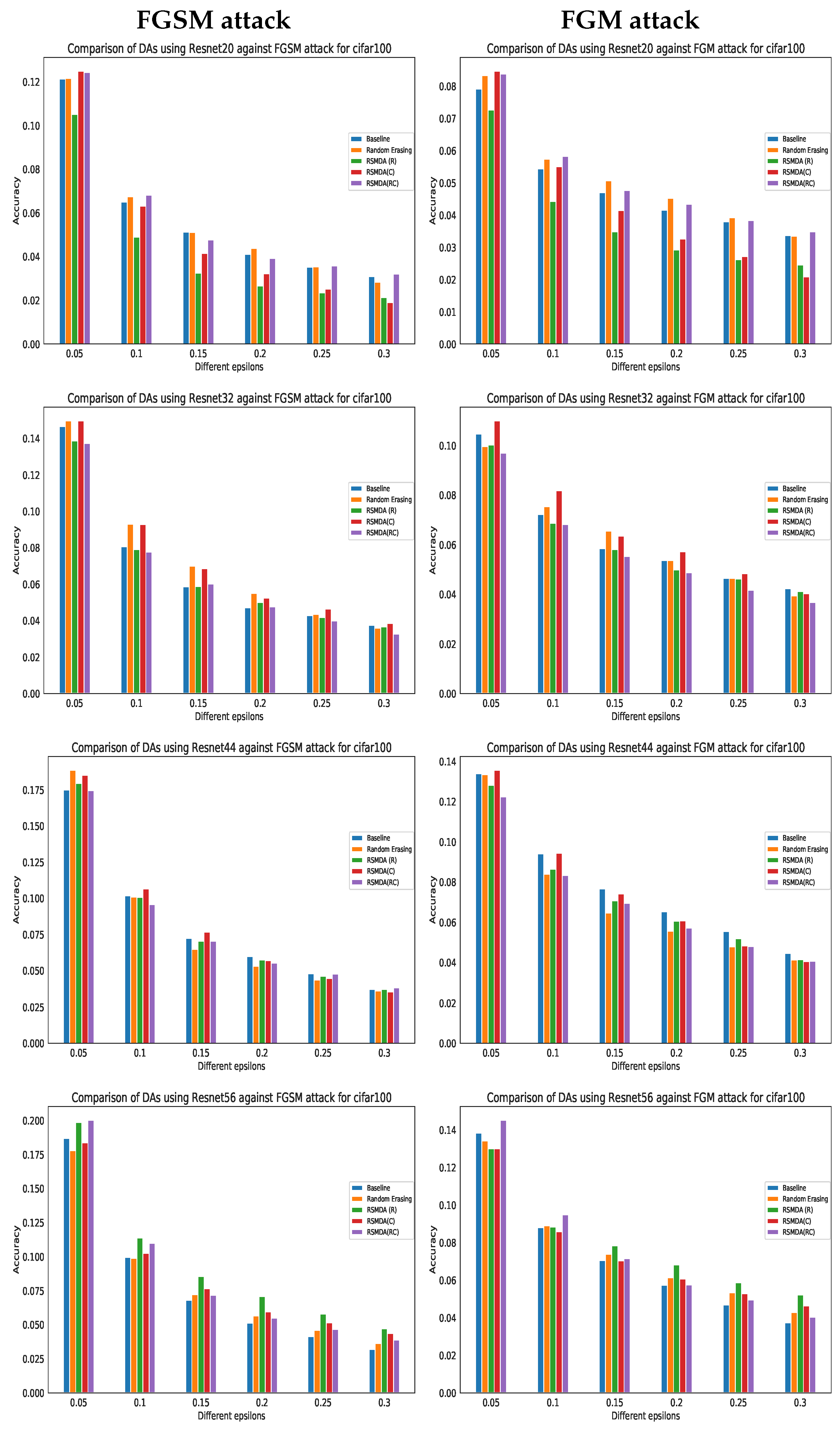
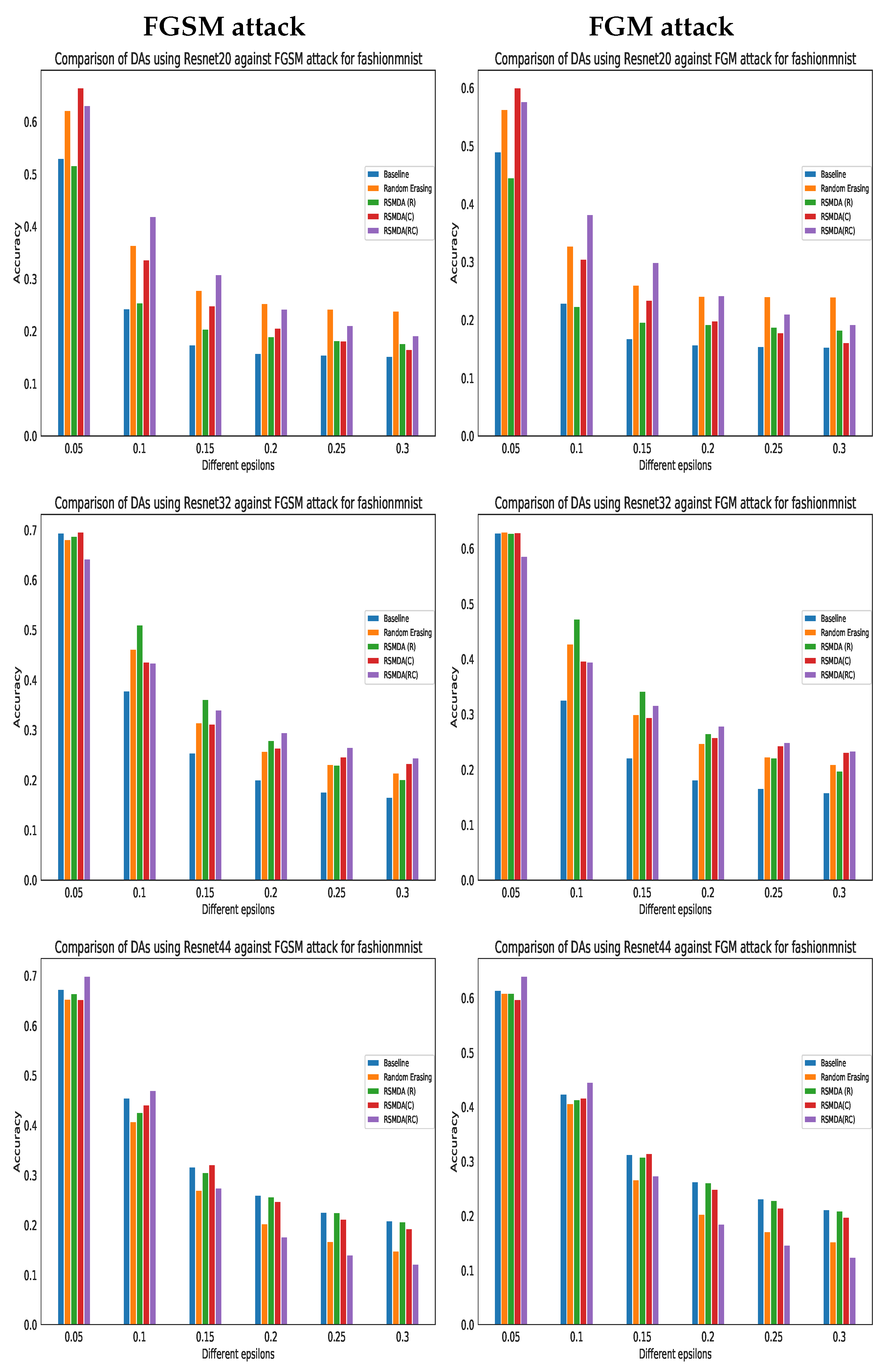
4.3.3. Adversarial Attacks

Deep networks are fooled by adding a small unrecognizable perturbation to the input data, and the perturbed data mislead the network to degrade the performance; this whole mechanism is referred to as an adversarial attack [54,55]. A simple way to prevent an attack is to generate an unseen input sample [56]. For adversarial attacks, we assume that the attacker has complete information about the model, i.e., a white box attack. We use different pre-trained (all models trained by us) ResNet models for cifar10, cifar100, and fashionMNIST. In this section, we evaluate the robustness of the proposed approach due to directly dealing with the input data following the previous methods [36]. In order to check the robustness, we compare our three strategies with the baseline and random erasing performance against two adversarial attacks, namely, the fast gradient sign method (FGSM) [54] and the FGSM variant, fast gradient magnitude (FGM) [54,57], was proposed to alleviate the issue of noise perceptibility [57]. These two attacks, FGSM and FGM, were used to check robustness using different datasets and models. In all adversarial experiments, we used the baseline, random erasing, and the model trained by the three proposed strategies against these attacks using different values of epsilon [54], i.e., [0.05, 0.1, 0.15, 0.2, 0.25, 0.3]. In Figure 4, Figure 5 and Figure 6, the x-axis values and y-axis values show epsilon and accuracy, respectively. For the CIFAR10 dataset, we check the robustness against three strategies and compare it with the baseline and random erasing using different trained models of ResNet. In Figure 4, it can be seen that in the case of ResNet20 and ResNet44, interestingly, RSMDA(C) was more robust against both attacks than the others, while in the case of ResNet20 and ResNet56, RSMDA(R) was the winner. Overall, the proposed approach beats the baseline and random erasing.

For the CIFAR100 dataset, we repeat the same experiment pattern to check the behavior of the robustness using a dataset with a large number of classes. We checked the robustness using the CIFAR100 dataset. The pattern was very much different than what we discussed in the cifar10 case. As shown in Figure 5, RSMDA(RC) was more robust using the ResNet20 and ResNet56 models, and RSMDA(C) was more successful using ResNet32 and ResNet44. In all of the models’ cases, the proposed approach shows more robustness compared to the baseline and random erasing.

To check the behavior of the robustness of the grayscale dataset, we use the trained models on fashionMNIST against these adversarial attacks. We repeated the same stream of experiments, as shown in Figure 6. Surprisingly, the fashionMNIST case showed very different behavior from what was discussed in the cifar10 and cifar100 cases. In Figure 6, the overall RSMDA(RC) is more robust using the ResNet20 and ResNet44 models, and RSMDA(R) is more robust with ResNet32. The proposed approach also showed more robustness with the grayscale dataset.

Overall, the proposed approach is more robust. In rare cases, random erasing showed more robustness, such as with ResNet44 at an epsilon value of 0.05 in the cifar100 case (as shown in Figure 5), but, with an increase in the value of epsilon, it becomes less robust. The proposed approach’s robustness not only checks in the case of different numbers of classes but also checks in different color domain datasets. In both the grayscale and color datasets, it significantly improves the robustness against adversarial attacks, except in some very rare cases.

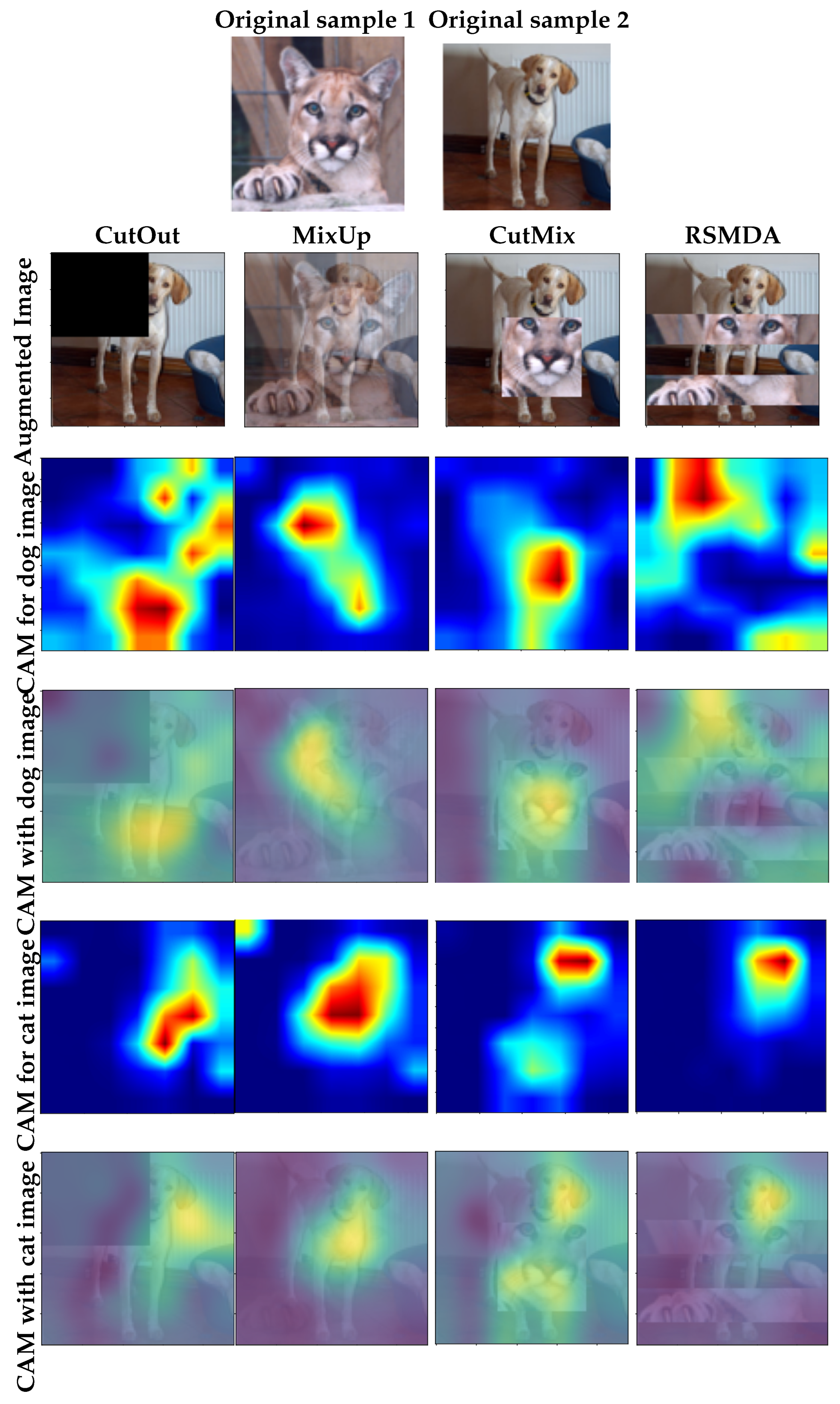
4.3.4. Class Activation Map (CAM)

Class activation maps (https://github.com/chaeyoung-lee/pytorch-CAM [58,59,60], accessed on 10 September 2022) highlight different object regions of interest. They are plotted from the final layer of the convolutional neural network [59]. They help us to know where the model focuses more to ascertain whether the model is actually learning the discriminating features or not. We compare this with relevant data augmentations, including CutOut, CutMix, and MixUp, to check whether RSMDA is really learning the discriminating features for two objects from their respective incomplete views. For this purpose, first, we take two images, i.e., the cat and dog shown in the first row of Figure 7. In the second row of Figure 7, we prepare the augmented output as an input for the model. Then, we use ResNet50 (https://pytorch.org/hub/nvidia_deeplearningexamples_resnet50/, accessed on 10 September 2022), a pre-trained model, to obtain the CAM for each augmented input. In the third and fourth rows of Figure 7, only the CAM for the dog and the CAM with the dog are shown, respectively, to clearly show where the model focuses more. The same is repeated for the cat class in the fifth and sixth rows. RSMDA suggests that it learns features that are clear to the model, i.e., the tail of the dog where the model focuses more on dog classification. We believe such tiny features are quite helpful for models to recognize objects. Among these four augmentations, CutMix has a strong capability to capture features, as shown in the third column of Figure 7. From the experiments, it seems that RSMDA has the capability to learn tiny or small features that are quite helpful for models in recognizing objects.

5. Conclusions

In conclusion, we are the first to propose a novel data augmentation technique, named random slices mixing data augmentation (RSMDA), to deal with feature loss problems in single-image data augmentation techniques. RSMDA mixes two images uniquely in a sliced way. Furthermore, we proposed and investigated three different strategies of RSMDA, namely, RSMDA row-wise (horizontally), RSMDA column-wise (vertically), and RSMDA row–column-wise based on binary randomness. Among these strategies, RSMDA row-wise showed a significant performance in terms of accuracy and robustness. We also found the best parameters of the proposed approach: slice size and probability. Using different datasets and models, overall, RSMDA has shown better performance than single- and multi-image data augmentation methods. We also checked the robustness of RSMDA in detail, and it improves robustness over the baseline and random erasing. Finally, we drew CAM to analyze the model focus, and it was found that the model focuses on tiny and quite helpful features. These tiny features are very important in object recognition, so RSMDA has its importance in object recognition. In the future, we will explore different slice shapes, such as triangular, circular, and elliptical, rather than only rectangular. Additionally, we may explore the same approach for only salient parts of the images.

References

1. Kumar, J.; Bedi, P.; Goyal, S.; Shrivastava, A.; Kumar, S. Novel Algorithm for Image Classification Using Cross Deep Learning Technique. IOP Conf. Ser. Mater. Sci. Eng. 2021, 1099, 012033. [Google Scholar] [CrossRef]
2. Liu, J.; An, F. Image classification algorithm based on deep learning-kernel function. Sci. Program. 2020, 2020, 7607612. [Google Scholar] [CrossRef] [Green Version]
3. Wang, H.; Meng, F. Research on power equipment recognition method based on image processing. EURASIP J. Image Video Process. 2019, 2019, 57. [Google Scholar] [CrossRef]
4. Kumar, T.; Turab, M.; Talpur, S.; Brennan, R.; Bendechache, M. Forged Character Detection Datasets: Passports, Driving Licences And Visa Stickers. Int. J. Artif. Intell. Appl. (IJAIA) 2022, 13, 21–35. [Google Scholar] [CrossRef]
5. Ciresan, D.; Meier, U.; Masci, J.; Gambardella, L.; Schmidhuber, J. Flexible, high performance convolutional neural networks for image classification. In Proceedings of the Twenty-Second International Joint Conference on Artificial Intelligence, Catalonia, Spain, 16–22 July 2011. [Google Scholar]
6. Kumar, T.; Park, J.; Ali, M.; Uddin, A.; Ko, J.; Bae, S. Binary-classifiers-enabled filters for semi-supervised learning. IEEE Access 2021, 9, 167663–167673. [Google Scholar] [CrossRef]
7. Khan, W.; Raj, K.; Kumar, T.; Roy, A.; Luo, B. Introducing urdu digits dataset with demonstration of an efficient and robust noisy decoder-based pseudo example generator. Symmetry 2022, 14, 1976. [Google Scholar] [CrossRef]
8. Chandio, A.; Gui, G.; Kumar, T.; Ullah, I.; Ranjbarzadeh, R.; Roy, A.; Hussain, A.; Shen, Y. Precise single-stage detector. arXiv 2022, arXiv:2210.04252. [Google Scholar]
9. Kumar, T.; Park, J.; Ali, M.; Uddin, A.; Bae, S. Class Specific Autoencoders Enhance Sample Diversity. J. Broadcast Eng. 2021, 26, 844–854. [Google Scholar]
10. Roy, A.; Bhaduri, J.; Kumar, T.; Raj, K. A Computer Vision-Based Object Localization Model for Endangered Wildlife Detection. Ecol. Econ. Forthcom. 2022. [Google Scholar] [CrossRef]
11. Nanni, L.; Maguolo, G.; Brahnam, S.; Paci, M. An ensemble of convolutional neural networks for audio classification. Appl. Sci. 2021, 11, 5796. [Google Scholar] [CrossRef]
12. Hershey, S.; Chaudhuri, S.; Ellis, D.; Gemmeke, J.; Jansen, A.; Moore, R.; Plakal, M.; Platt, D.; Saurous, R.; Seybold, B. Others CNN architectures for large-scale audio classification. In Proceedings of the 2017 IEEE International Conference on Acoustics, Speech and Signal Processing (ICASSP), New Orleans, LA, USA, 5–9 March 2017; pp. 131–135. [Google Scholar]
13. Rong, F. Audio classification method based on machine learning. In Proceedings of the 2016 International Conference on Intelligent Transportation, Big Data & Smart City (ICITBS), Changsha, China, 17–18 December 2016; pp. 81–84. [Google Scholar]
14. Aiman, A.; Shen, Y.; Bendechache, M.; Inayat, I.; Kumar, T. AUDD: Audio Urdu Digits Dataset for Automatic Audio Urdu Digit Recognition. Appl. Sci. 2021, 11, 8842. [Google Scholar]
15. Turab, M.; Kumar, T.; Bendechache, M.; Saber, T. Investigating Multi-Feature Selection and Ensembling for Audio Classification. arXiv 2022, arXiv:2206.07511. [Google Scholar] [CrossRef]
16. Park, J.; Kumar, T.; Bae, S. Search for optimal data augmentation policy for environmental sound classification with deep neural networks. J. Broadcast Eng. 2020, 25, 854–860. [Google Scholar]
17. Singh, A.; Ranjbarzadeh, R.; Raj, K.; Kumar, T.; Roy, A. Understanding EEG signals for subject-wise Definition of Armoni Activities. arXiv 2023, arXiv:2301.00948. [Google Scholar]
18. Kolluri, J.; Razia, D.; Nayak, S. Text classification using machine learning and deep learning models. Int. Conf. Artif. Intell. Manuf. Renew. Energy (ICAIMRE) 2019. [Google Scholar] [CrossRef]
19. Minaee, S.; Kalchbrenner, N.; Cambria, E.; Nikzad, N.; Chenaghlu, M.; Gao, J. Deep learning–based text classification: A comprehensive review. ACM Comput. Surv. (CSUR) 2021, 54, 1–40. [Google Scholar] [CrossRef]
20. Nguyen, T.; Shirai, K. Text classification of technical papers based on text segmentation. In Proceedings of the International Conference on Application of Natural Language to Information Systems, Salford, UK, 19–21 Jun2013; pp. 278–284. [Google Scholar]
21. Shorten, C.; Khoshgoftaar, T. A survey on image data augmentation for deep learning. J. Big Data 2019, 6, 1–48. [Google Scholar] [CrossRef]
22. Kukačka, J.; Golkov, V.; Cremers, D. Regularization for deep learning: A taxonomy. arXiv 2017, arXiv:1710.10686. [Google Scholar]
23. Ioffe, S.; Szegedy, C. Batch normalization: Accelerating deep network training by reducing internal covariate shift. In Proceedings of the International Conference on Machine Learning, Lille, France, 6–11 July 2015; pp. 448–456. [Google Scholar]
24. Srivastava, N.; Hinton, G.; Krizhevsky, A.; Sutskever, I.; Salakhutdinov, R. Dropout: A simple way to prevent neural networks from overfitting. J. Mach. Learn. Res. 2014, 15, 1929–1958. [Google Scholar]
25. Zhong, Z.; Zheng, L.; Kang, G.; Li, S.; Yang, Y. Random erasing data augmentation. Proc. Aaai Conf. Artif. Intell. 2020, 34, 13001–13008. [Google Scholar] [CrossRef]
26. Simonyan, K.; Zisserman, A. Very deep convolutional networks for large-scale image recognition. arXiv 2014, arXiv:1409.1556. [Google Scholar]
27. Takahashi, R.; Matsubara, T.; Uehara, K. Data augmentation using random image cropping and patching for deep CNNs. IEEE Trans. Circuits Syst. Video Technol. 2019, 30, 2917–2931. [Google Scholar] [CrossRef] [Green Version]
28. Mikołajczyk, A.; Grochowski, M. Data augmentation for improving deep learning in image classification problem. In Proceedings of the 2018 International Interdisciplinary PhD Workshop (IIPhDW), Swinoujscie, Poland, 9–12 May 2018; pp. 117–122. [Google Scholar]
29. Chen, S.; Dobriban, E.; Lee, J. A group-theoretic framework for data augmentation. Adv. Neural Inf. Process. Syst. 2020, 33, 21321–21333. [Google Scholar]
30. Wei, J.; Zou, K. Eda: Easy data augmentation techniques for boosting performance on text classification tasks. arXiv 2019, arXiv:1901.11196. [Google Scholar]
31. Acción, Á.; Argüello, F.; Heras, D. Dual-window superpixel data augmentation for hyperspectral image classification. Appl. Sci. 2020, 10, 8833. [Google Scholar] [CrossRef]
32. Singh, K.; Yu, H.; Sarmasi, A.; Pradeep, G.; Lee, Y. Hide-and-seek: A data augmentation technique for weakly-supervised localization and beyond. arXiv 2018, arXiv:1811.02545. [Google Scholar]
33. Chen, P.; Liu, S.; Zhao, H.; Jia, J. Gridmask data augmentation. arXiv 2020, arXiv:2001.04086. [Google Scholar]
34. DeVries, T.; Taylor, G. Improved regularization of convolutional neural networks with cutout. arXiv 2017, arXiv:1708.04552. [Google Scholar]
35. Zhang, H.; Cisse, M.; Dauphin, Y.; Lopez-Paz, D. mixup: Beyond empirical risk minimization. arXiv 2017, arXiv:1710.09412. [Google Scholar]
36. Yun, S.; Han, D.; Oh, S.; Chun, S.; Choe, J.; Yoo, Y. Cutmix: Regularization strategy to train strong classifiers with localizable features. In Proceedings of the IEEE/CVF International Conference on Computer Vision, Seoul, Korea, 27–28 October 2019; pp. 6023–6032. [Google Scholar]
37. Summers, C.; Dinneen, M. Improved mixed-example data augmentation. In Proceedings of the 2019 IEEE Winter Conference on Applications of Computer Vision (WACV), Waikoloa Village, HI, USA, 7–11 January 2019; pp. 1262–1270. [Google Scholar]
38. Kumar, T.; Brennan, R.; Bendechache, M. Slices Random Erasing Augmentation. Available online: https://d1wqtxts1xzle7.cloudfront.net/87590566/csit120201-libre.pdf?1655368573=&response-content-disposition=inline%3B+filename%3DSTRIDE_RANDOM_ERASING_AUGMENTATION.pdf&Expires=1674972117&Signature=ThC7JbxC8jJzEQPchixX86VpZwMkalCENMNEEsXuvgtfKsqVspfmkEM89XXh1cjd1PnUAzJbHAw2Gf4WTG7-WD8VzmQwiyuJ3u~ADfswlhW6wb51n2VTgU6M3hLhQFGgWVlUbUUqptbttUU12Nw0QYekjw3fUjm2eS23phjn2HismJS05IcVB6QRyXXUKq1ie2XTRDGixUZLqZCi5OFBCaro5GBZXPMgn1XkJOqKVGDvRTEjgykzgoWx-sZXc0RwUi7CteyXM3YEJM3K2uTFz~wI0OOa8Ff~aEHfiLBGcWASq1Z6aGRtVrDUaXBiSSWD~OcgwlnNW~nKSSzjaegZuQ&Key-Pair-Id=APKAJLOHF5GGSLRBV4ZA (accessed on 8 December 2022).
39. Krizhevsky, A.; Sutskever, I.; Hinton, G. Imagenet classification with deep convolutional neural networks. Commun. ACM 2017, 60, 84–90. [Google Scholar] [CrossRef] [Green Version]
40. He, K.; Zhang, X.; Ren, S.; Sun, J. Deep residual learning for image recognition. In Proceedings of the IEEE Conference on Computer Vision and Pattern Recognition, Las Vegas, NV, USA, 27–30 June 2016; pp. 770–778. [Google Scholar]
41. Hinton, G.; Srivastava, N.; Krizhevsky, A.; Sutskever, I.; Salakhutdinov, R. Improving neural networks by preventing co-adaptation of feature detectors. arXiv 2012, arXiv:1207.0580. [Google Scholar]
42. Ba, J.; Frey, B. Adaptive dropout for training deep neural networks. Adv. Neural Inf. Process. Syst. 2013, 26. [Google Scholar]
43. Wan, L.; Zeiler, M.; Zhang, S.; Le Cun, Y.; Fergus, R. Regularization of neural networks using dropconnect. Int. Conf. Mach. Learn. 2013, 28, 1058–1066. [Google Scholar]
44. Zeiler, M.; Fergus, R. Stochastic pooling for regularization of deep convolutional neural networks. arXiv 2013, arXiv:1301.3557. [Google Scholar]
45. Tompson, J.; Goroshin, R.; Jain, A.; LeCun, Y.; Bregler, C. Efficient object localization using convolutional networks. In Proceedings of the IEEE Conference on Computer Vision and Pattern Recognition, Boston, Ma, USA, 7–12 June 2015; pp. 648–656. [Google Scholar]
46. Han, D.; Kim, J.; Kim, J. Deep pyramidal residual networks. In Proceedings of the IEEE Conference on Computer Vision and Pattern Recognition, Honolulu, HI, USA, 21–26 July 2017; pp. 5927–5935. [Google Scholar]
47. Krizhevsky, A.; Hinton, G. Others Learning Multiple Layers of Features from Tiny Images. Master’s Thesis, University of Tront, Toronto, ON, Canada, 2009. [Google Scholar]
48. Coates, A.; Ng, A.; Lee, H. An analysis of single-layer networks in unsupervised feature learning. In Proceedings of the Fourteenth International Conference on Artificial Intelligence and Statistics, Fort Lauderdale, FL, USA, 11–13 April 2011; pp. 215–223. [Google Scholar]
49. Xiao, H.; Rasul, K.; Vollgraf, R. Fashion-mnist: A novel image dataset for benchmarking machine learning algorithms. arXiv 2017, arXiv:1708.07747. [Google Scholar]
50. Huang, G.; Sun, Y.; Liu, Z.; Sedra, D.; Weinberger, K. Deep networks with stochastic depth. Eur. Conf. Comput. Vis. 2016, 9908, 646–661. [Google Scholar]
51. Szegedy, C.; Vanhoucke, V.; Ioffe, S.; Shlens, J.; Wojna, Z. Rethinking the inception architecture for computer vision. In Proceedings of the IEEE Conference on Computer Vision and Pattern Recognition, Las Vegas, NV, USA, 27–30 June 2016; pp. 2818–2826. [Google Scholar]
52. Verma, V.; Lamb, A.; Beckham, C.; Najafi, A.; Mitliagkas, I.; Lopez-Paz, D.; Bengio, Y. Manifold mixup: Better representations by interpolating hidden states. Int. Conf. Mach. Learn. 2019, 97, 6438–6447. [Google Scholar]
53. Yamada, Y.; Iwamura, M.; Akiba, T.; Kise, K. Shakedrop regularization for deep residual learning. IEEE Access 2019, 7, 186126–186136. [Google Scholar] [CrossRef]
54. Goodfellow, I.; Shlens, J.; Szegedy, C. Explaining and harnessing adversarial examples. arXiv 2014, arXiv:1412.6572. [Google Scholar]
55. Szegedy, C.; Zaremba, W.; Sutskever, I.; Bruna, J.; Erhan, D.; Goodfellow, I.; Fergus, R. Intriguing properties of neural networks. arXiv 2013, arXiv:1312.6199. [Google Scholar]
56. Madry, A.; Makelov, A.; Schmidt, L.; Tsipras, D.; Vladu, A. Towards deep learning models resistant to adversarial attacks. arXiv 2017, arXiv:1706.06083. [Google Scholar]
57. Agarwal, A.; Singh, R.; Vatsa, M. The Role of’Sign’and’Direction’of Gradient on the Performance of CNN. In Proceedings of the IEEE/CVF Conference on Computer Vision and Pattern Recognition Workshops, Seattle, WA, USA, 14–19 June 2020; pp. 646–647. [Google Scholar]
58. Zhou, B.; Khosla, A.; Lapedriza, A.; Oliva, A.; Torralba, A. Learning deep features for discriminative localization. In Proceedings of the IEEE Conference on Computer Vision and Pattern Recognition, Honolulu, HI, USA, 21–26 July 2016; pp. 2921–2929. [Google Scholar]
59. Jiang, P.; Zhang, C.; Hou, Q.; Cheng, M.; Wei, Y. Layercam: Exploring hierarchical class activation maps for localization. IEEE Trans. Image Process. 2021, 30, 5875–5888. [Google Scholar] [CrossRef] [PubMed]
60. Jung, H.; Oh, Y. Towards better explanations of class activation mapping. In Proceedings of the IEEE/CVF International Conference on Computer Vision, Montreal, BC, Canada, 11–17 October 2021; pp. 1336–1344. [Google Scholar]
Figure 1. Comparison of different data augmentations against the proposed RSMDA.
Applsci 13 01711 g001
Figure 2. Three strategies for Random Slices Mixing Data Augmentation (RSMDA).
Applsci 13 01711 g002
Figure 3. Hyperparameters: probability and slice size effect on accuracy.
Applsci 13 01711 g003
Figure 4. Comparison of DAs against different adversarial attacks for CIFAR10 dataset using different models.
Applsci 13 01711 g004
Figure 5. Comparison of DAs against different adversarial attacks for CIFAR100 dataset using different models.
Applsci 13 01711 g005
Figure 6. Comparison of DAs against different adversarial attacks for fashionMNIST dataset using different models.
Applsci 13 01711 g006
Figure 7. Data augmentation visualizations comparison.
Applsci 13 01711 g007