Article

Stochastic Weight Averaging Revisited

Research Center for Applied Mathematics and Machine Intelligence, Zhejiang Lab, Hangzhou 311121, China
*
Author to whom correspondence should be addressed.
Appl. Sci. 2023, 13(5), 2935; https://doi.org/10.3390/app13052935
Submission received: 27 October 2022 / Revised: 13 February 2023 / Accepted: 23 February 2023 / Published: 24 February 2023

Abstract

:
Averaging neural network weights sampled by a backbone stochastic gradient descent (SGD) is a simple-yet-effective approach to assist the backbone SGD in finding better optima, in terms of generalization. From a statistical perspective, weight-averaging contributes to variance reduction. Recently, a well-established stochastic weight-averaging (SWA) method was proposed, which featured the application of a cyclical or high-constant (CHC) learning-rate schedule for generating weight samples for weight-averaging. Then, a new insight on weight-averaging was introduced, which stated that weight average assisted in discovering a wider optima and resulted in better generalization. We conducted extensive experimental studies concerning SWA, involving 12 modern deep neural network model architectures and 12 open-source image, graph, and text datasets as benchmarks. We disentangled the contributions of the weight-averaging operation and the CHC learning-rate schedule for SWA, showing that the weight-averaging operation in SWA still contributed to variance reduction, and the CHC learning-rate schedule assisted in exploring the parameter space more widely than the backbone SGD, which could be be under-fitted due to a lack of training budget. We then presented an algorithm termed periodic SWA (PSWA) that comprised a series of weight-averaging operations to exploit such wide parameter space structures as explored by the CHC learning-rate schedule, and we empirically demonstrated that PSWA outperformed its backbone SGD remarkably.

1. Introduction

A stochastic gradient descent (SGD) equipped with a decaying learning-rate schedule is the de facto approach for training modern deep neural networks (DNNs). Averaging neural network (NN) weights sampled by a backbone SGD has shown to be a simple-yet-effective approach to assist the backbone SGD in identifying better optima, in terms of generalization. The concept of weight-averaging, also referred to as iterate-averaging or tail-averaging [1], was introduced by [2,3]. A weight-averaging procedure averages the final few iterates of an SGD. From a statistical perspective, it has been proved that the weight-averaging operation contributed to decreasing the variance in the final iterate of its backbone SGD, resulting in a stabilizing effect in terms of regularization properties and prediction guarantees [4]. We referred to this view as variance reduction in this article.
Recently, a stochastic weight-averaging (SWA) method was proposed that attracted much attention in the field. It was easy to implement yet could improve SGD in order to achieve better generalization results without significant computational demand [5,6,7]. SWA starts after a converged SGD (namely, the backbone SGD), which outputs a local optimum w SGD of the loss function f ( w ) , where w denotes the NN weights. In the SWA process, another backbone SGD procedure is run, starting at w SGD . This new SGD process employs a cyclical or high-constant (CHC) learning-rate schedule. The application of the CHC learning-rate schedule is a major feature that discriminates SWA from other weight-averaging methods. Novel local optima are sampled along the trajectory of this new SGD process. Then, a weight-averaging operation is used, which outputs the mean of the optima, denoted by w SWA , as the final output of SWA. A pseudo-code to implement SWA is shown in Algorithm 1, which outputs a running average of the sampled weights per c iterations.
Algorithm 1 Stochastic Weight Averaging (SWA)
Input: weights w SGD , learning-rate schedule, cycle length c, number of iterations n
Output: w SWA
 1:
w w SGD ; w SWA w .
 2:
for i 1 , 2 , , n do
 3:
    Compute current learning rate α according to the learning-rate schedule.
 4:
     w w α L i ( w ) (stochastic gradient update).
 5:
    if mod(i,c) = 0 then
 6:
         n models i / c (number of models averaged).
 7:
         w SWA w SWA · n models + w / n models + 1 .
 8:
    end if
 9:
end for
10:
return w SWA
A common insight to explain SWA’s success is that the local optima it discovers are located at the boundary of a high-quality basin region in the DNN weight parameter space. Conducting weight-averaging over such optima then resulted in a wider optimum that is closer to the center of the basin region [5], and a wider optimum leads to better generalization [5,8].

1.1. Limitations

As mentioned previously, there are two seemingly independent views on the role of weight-averaging: one is statistical, namely, the variance-reduction perspective; and the other is geometric, namely, the wider-optimum perspective. However, we were unaware of nature of the relationship between these two views, and how to reconcile them. After a detailed inspection of SWA [5], we discovered that its behavior resulted from a combined effect of several possible intertwined factors, namely the convergence rate of the SGD that processed before SWA, the CRC learning-rate schedule, the weight-averaging operation, and finally, the application of the momentum technique and weight-decaying. The common geometric view could not explain the specific role of each factor. For example, it could not answer the following questions:
  • If we did not use the momentum technique in its backbone SGD, how would SWA behave?
  • If the SGD that processed before SWA could not converge or converged to a bad optimum, could SWA still work?
  • What was the actual function of the weight-averaging operation in SWA, either variance reduction, the identification of a wider optimum, or both?

1.2. Contributions

The previous concerns motivated us to revisit SWA. As SWA is a fundamental, generic, architecture-agnostic technique for training DNNs, any new findings or insights from this re-inspection could provide a broad potential impact on deep learning. The major contributions of this paper could be summarized, as follows:
  • We disentangled the contributions of the weight-averaging operation, the CHC learning-rate schedule, the application of momentum and weight decaying, and the rate at which the preceding SGD converged, to the behavior of SWA.
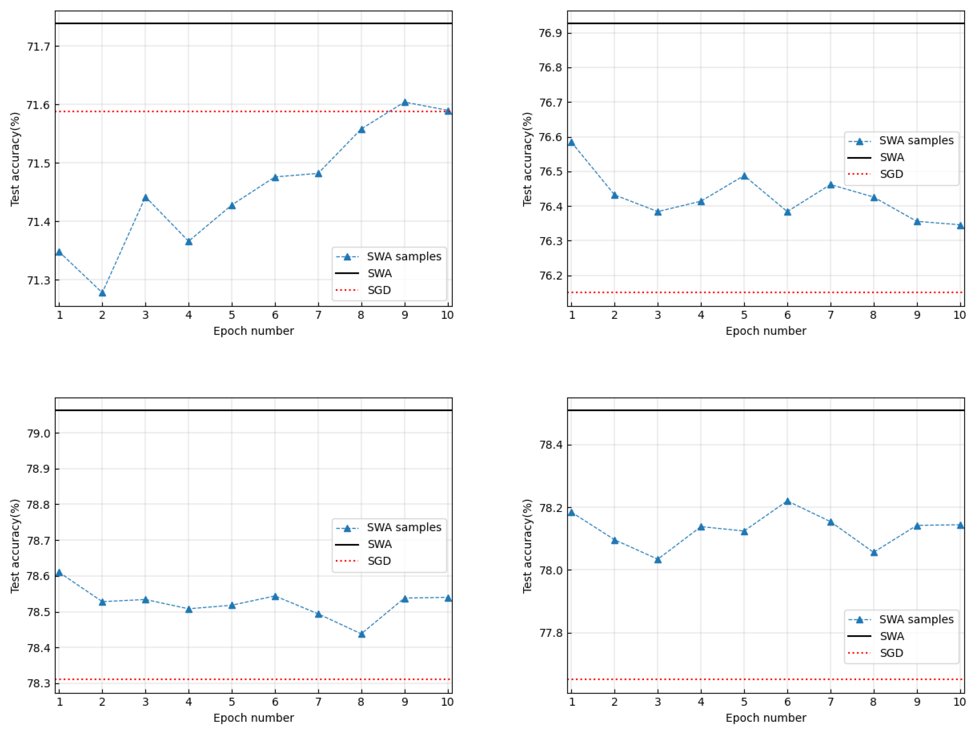
  • We found that the actual function of the weight-averaging operation in SWA was variance reduction, similar to tail-averaging [1].
  • We found cases in which SWA failed to discover better optima than its backbone SGD.
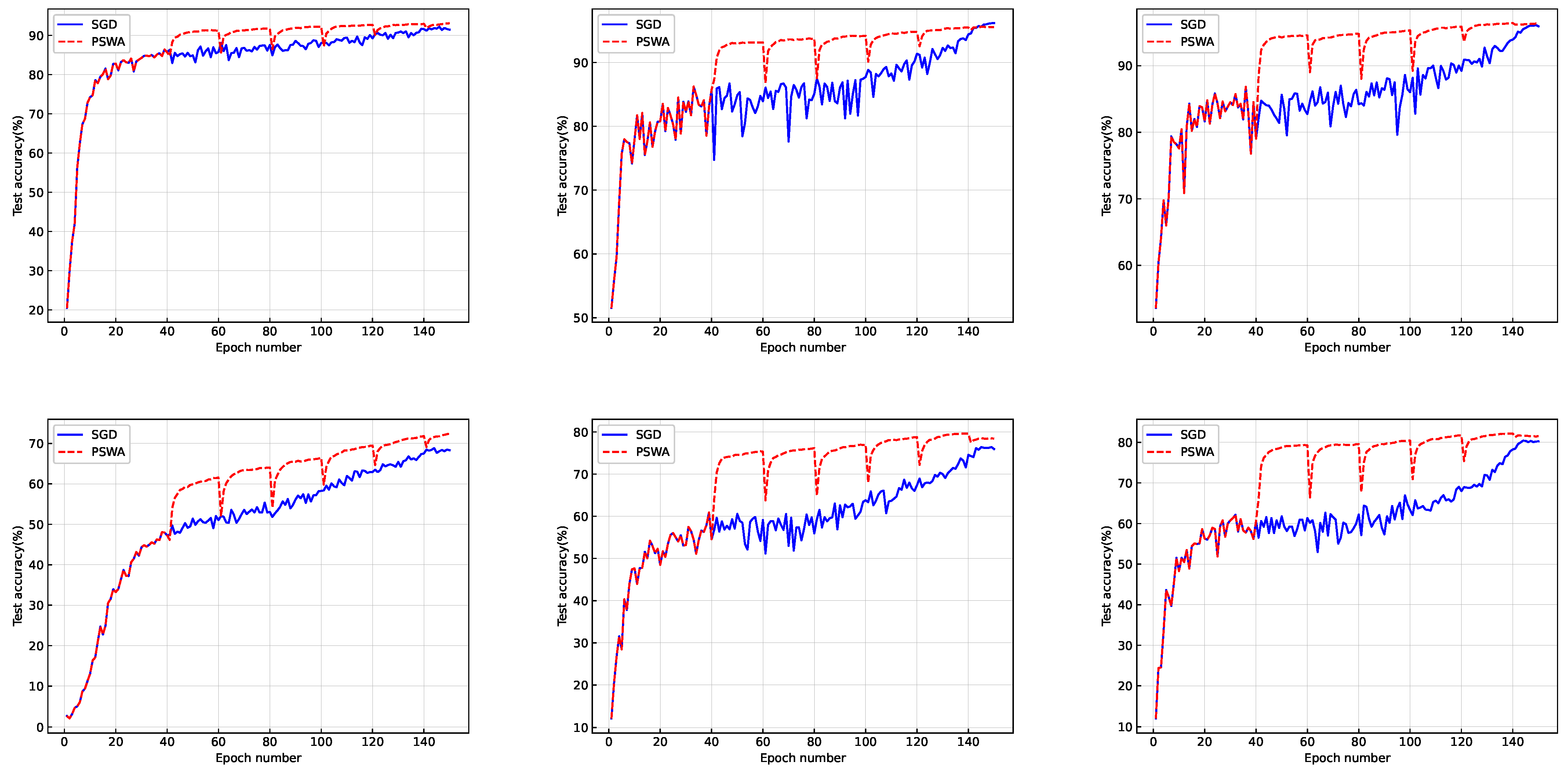
  • We found that SWA explored the parameter space more widely than its backbone SGD algorithm, which could be under-fitted due to a lack in the training budget. Inspired by this finding, we proposed a novel algorithm design, termed periodic SWA (PSWA), and demonstrated that it was preferable to SGD when the training budget was limited to the point it could not support the convergence of SGD.

2. Related Work

Here, we briefly introduce related works in the literature. A summary of their respective advantages and disadvantages is presented in Table 1.

2.1. Iterate Averaging

The basic concept of iterate averaging, also referred to as tail-averaging in [1], was introduced by [2,3]. The tail-averaging method averages the final few iterates of SGD. Therefore, it decreases the variance in the final iterate of SGD and stabilizes the regularization properties and prediction guarantees [4]. A generalization error boundary for tail-averaging within the context of least squares regression with the stochastic approximation was derived in [1].We show in this paper that the weight-averaging operation is a type of tail-averaging, which provides a stabilizing effect and the function of variance reduction for SWA.

2.2. Cyclical Learning Rates

The benefits of employing cyclical learning rates (CLRs) in an SGD procedure were demonstrated in [9,10]. In addition, a CLR strategy has been widely used for developing advanced DNN optimizers, such as fast geometric ensembles (FGE) [11], snapshot ensembles [12], super-convergence training [13], or exploring the loss landscape of DNNs [14]. In this paper, we discovered that the CLR strategy also plays a significant role in SWA’s success.

2.3. Convergence Theory

In [20], Zhu et al. presented a convergence theory for training DNNs, based on two assumptions: the input data points were distinct and the DNN architecture was over-parameterized. This theory suggests that, at least for fully connected NNs, convolutional NNs (CNNs), and residual NNs (ResNets), an SGD with a random weight initialization could attain 100% accuracy in classification tasks if the number of SGD iterations scales polynomially in the number of training samples and that of NN layers. Cheridito et al. demonstrated that for ReLU networks that had a much larger depth than their width, SGD failed to converge if the number of restarted SGD trajectories did not increase to infinity within a certain time frame [21]. Here, we investigated the specific roles of the CHC learning-rate schedule and the weight-averaging operation for promoting SGD’s convergence. While our results were empirical, they could promote more theoretical research on DNN convergence.

2.4. Loss Landscape Study & Sharpness-Aware Minimization

Another commonly used way to investigate the convergence problem has been through a loss-landscape analysis. The Hessian spectrum analysis was shown to be an effective approach to inspect smoothness, curvature, and sharpness in NN loss landscapes [15,16]. Yao et al. developed an open-source scalable framework for the fast computation of Hessian information in DNNs [17]. Typically, at least for some cases, NNs generalize better when they converge to a wider local optimum, and vice versa [8]. However, the correlation between the local sharpness of the loss landscape and a global property, such as generalization performance, could be only relational, instead of causative [18].
The empirical finding of the relationship between local sharpness and global generalization motivated the design of practical approaches for improving the generalization property of an SGD. For example, the sharpness-aware-minimization (SAM) method seeks NN weights that exist in a wider loss basin by optimizing the objective function to be sharpness-aware [19]. An SWA could be seen as a type of wideness-aware solver for DNN optimization. It was reported that SWA could find wider minima than SAM [6]. Our work characterized the root cause that led to SWA’s success and provided additional empirical evidence for an in-depth understanding of the loss landscape of DNNs.

2.5. Application Scenarios

Iterate-averaging, cyclical learning rates, loss-landscape studies, and SWA are all fundamental, generic, architecture-agnostic concepts that have been used for training DNNs. Therefore, potential application scopes of the aforementioned theories and techniques, along with this work, cover all scenarios to which deep-learning methods could contribute, such as speech recognition, image classification, information retrieval, reinforcement learning, etc.

3. Main Results

Our goal was to inspect the actual cause that led to SWA’s behavior. Towards this goal, we experimented with different DNN architectures on different datasets. We presented the main results indexed with questions concerning our interests. All details regarding the experimental settings are described in Appendix A.1.
Here, we adopted test accuracy as a measure of an algorithm’s generalization capability, according to [5]. In concept, test accuracy and an algorithm’s ability to generalize were not equivalent, since the latter denoted the difference between the test error and the training error. Nevertheless, for evaluating the generalization of SWA-type algorithms, test errors (or test accuracy) could act as qualified measures of generalization performance, since SWA and its backbone SGD, share the same training errors.

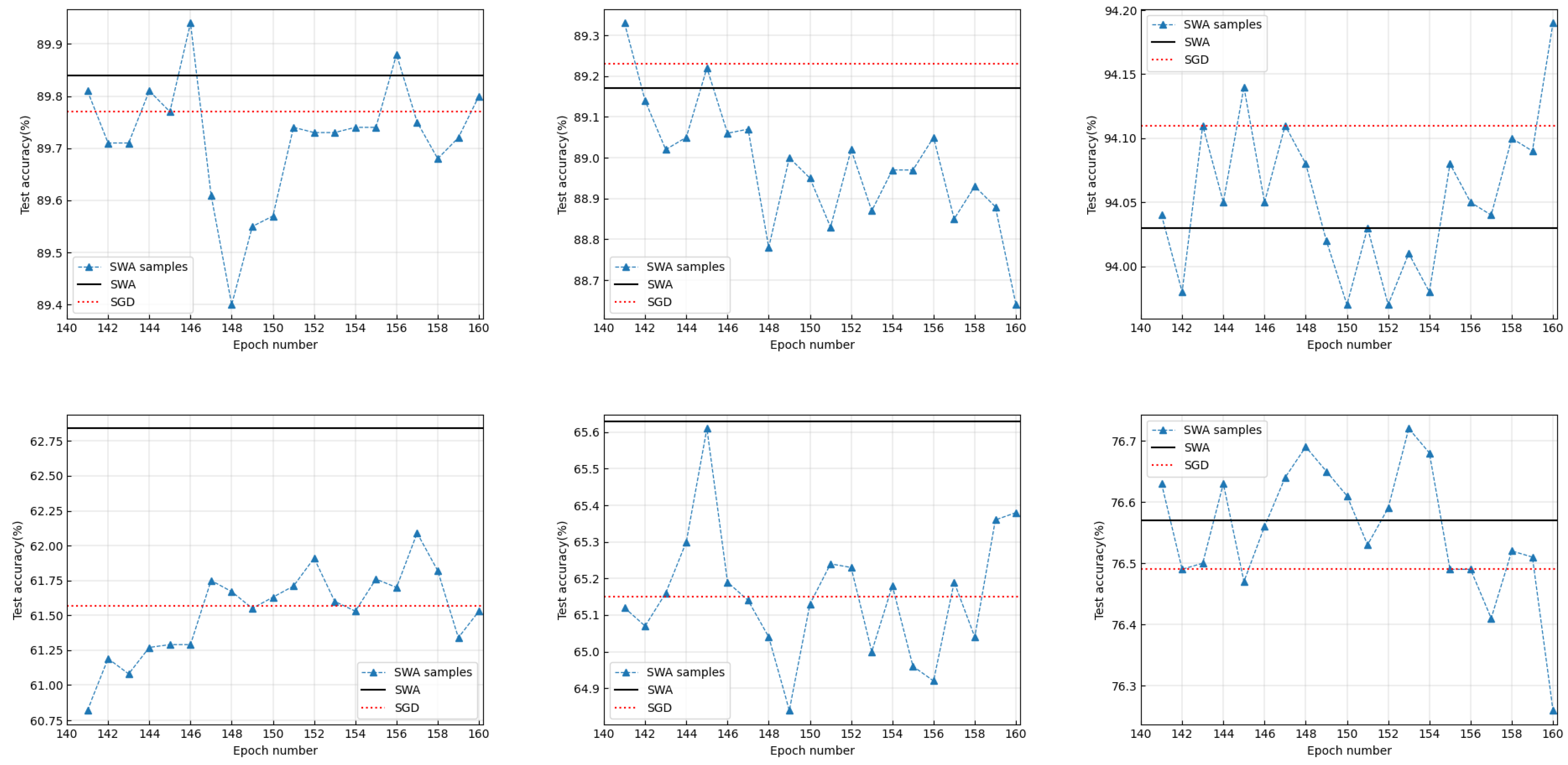
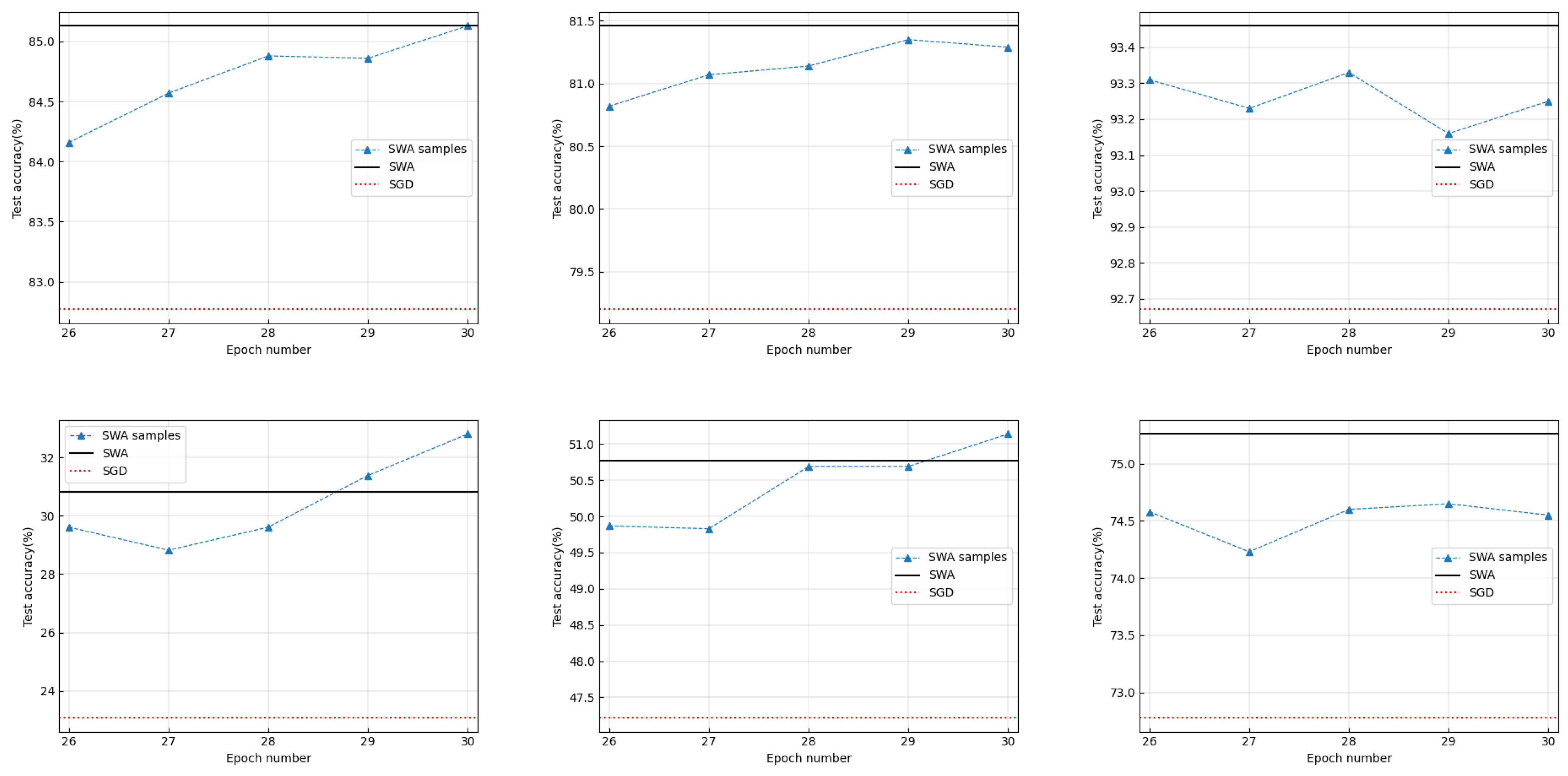
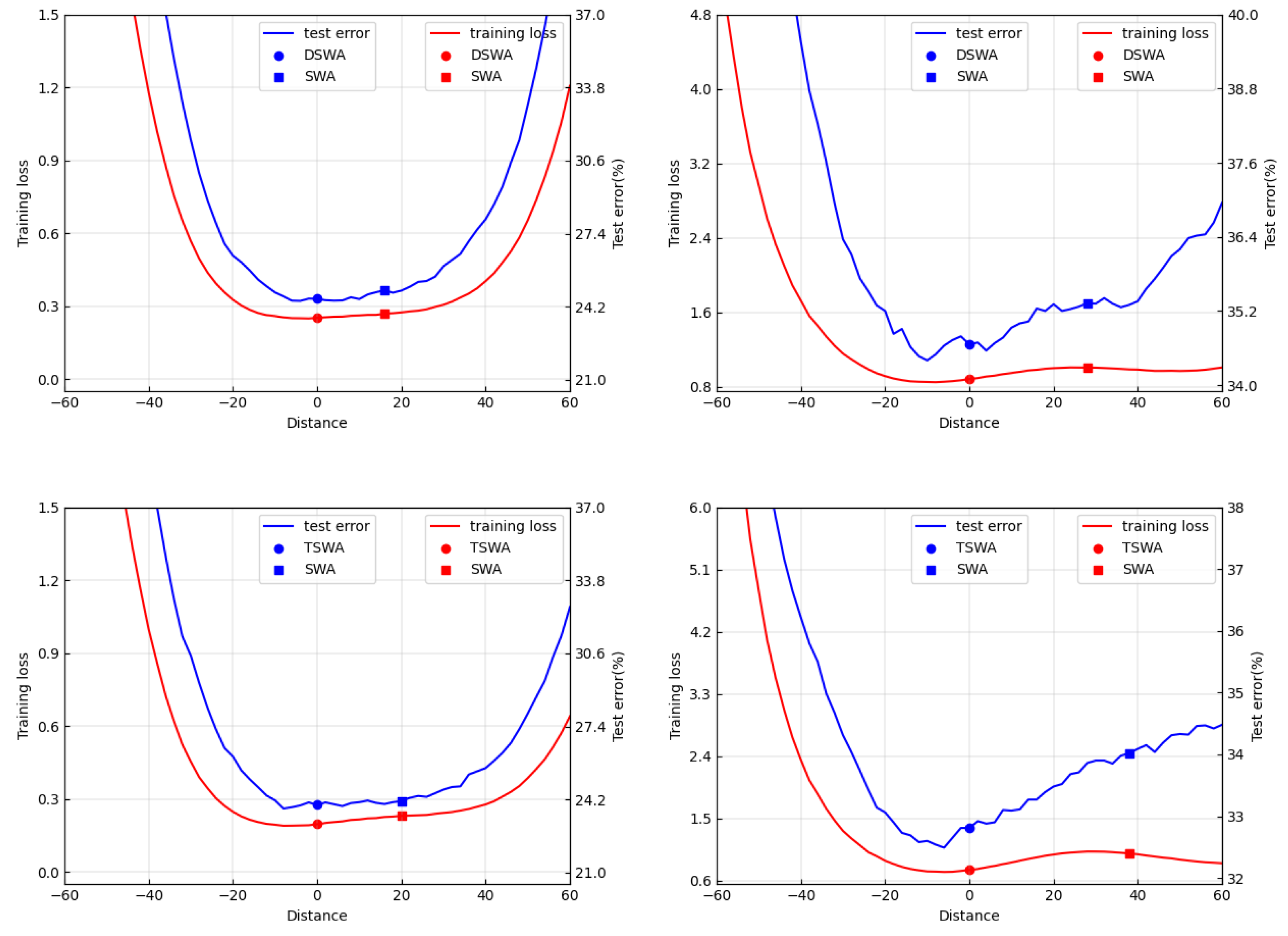
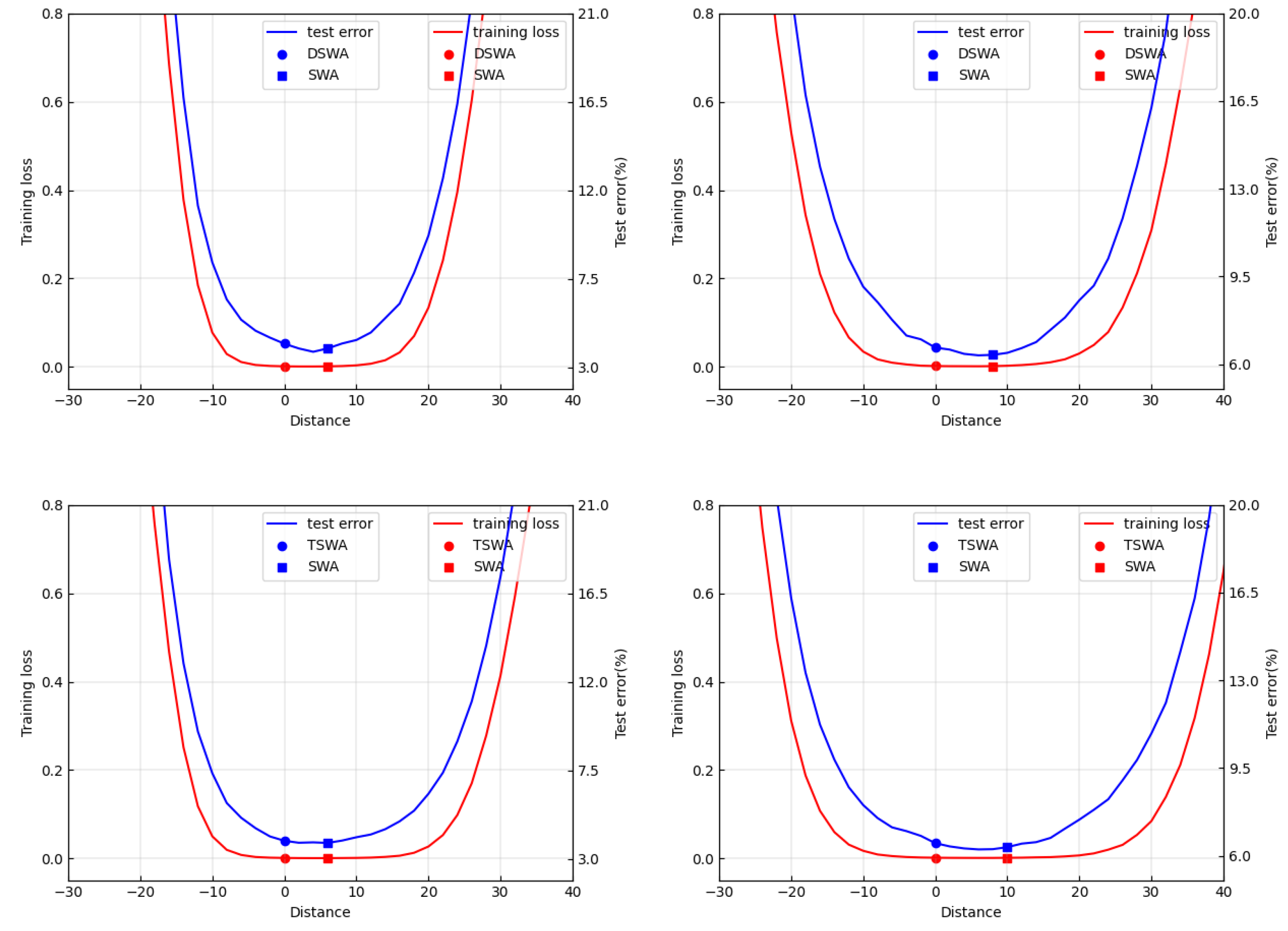
3.1. Does SWA Always Identify Wider Optima Than SGD?

The results reported in the SWA paper [5] showed that SGD generally converged to a boundary of a wide basin region and SWA assisted in finding an optimum exactly located in that wide basin region. All experiments conducted there used image datasets, such as CIFAR- { 10 , 100 } [22] and ImageNet ILSVRC-2012 [23,24]. We speculated whether SWA would always lead to a better generalization than an SGD. We conducted experiments on graph- and text-based datasets.The results showed that the answer was no, which further indicated that for these cases, SWA could not locate wider optima than an SGD. Specifically, on the graph dataset MUTAG, we used SWA to train a graph isomorphism network (GIN) for graph classification. The baseline optimizer selected was Adam, which is an advanced SGD method that performs better for graph-data-based tasks. We found that if we applied Adam with 300 epochs, then we obtained a test accuracy value of 89%; however, when we replaced Adam with SWA for the last 30 epochs, we obtained a smaller test accuracy value of 84%.
We considered the graph-node-classification task using graph-neural-network (GNN) models, such as a graph convolutional network (GCN) [25], GraphSAGE [26], and a graph attention network (GAT) [27], on public open-source datasets Cora, Citeseer, and Pubmed. The parameter setting for the experiment is shown in Table A1 in Appendix A.4. The test accuracy comparison result is presented in Table 2.
We also considered a graph-classification task using models MinCutPool [28] and SAGPool [29], on public open-source datasets NCI1 (https://paperswithcode.com/dataset/nci1, accessed on 1 November 2021), D&D (https://paperswithcode.com/sota/graph-classification-on-dd, accessed on 1 November 2021), and PROTEINS (https://paperswithcode.com/sota/graph-classification-on-proteins, accessed on 1 November 2021). The parameter settings are shown in Table A2, Table A3 and Table A4 in Appendix A.4. The test accuracy comparison result is shown in Table 3.
The experimental results for the graph datasets showed that using SWA did not always lead to a better generalization than other advanced SGD optimizers, such as Adam.
On a text dataset termed Microsoft Research Paraphrase Corpus (MRPC), we used an SGD with momentum to fine-tune the pre-trained model RoBERTa for testing whether two sentences were semantically equivalent. See details about the experimental setting in Appendix A.1.1. On average, the SGD provided a test accuracy value of 87.98% while SWA only achieved 87.50%.
We found that, even for image datasets, an SGD did not always converge to a boundary of a wide basin region, especially when we removed the momentum module from its backbone SGD. In such cases, we found that SWA could converge to a deep loss valley, where the averaged gradients over mini-batch training samples were all close to zero. Then, the products of such gradients and the learning rate were close to zero. In such cases, SWA failed to find a wider optimum with better generalization. See details of the experimental results in Appendix A.3.
To understand why removing the momentum module could result in SWA failing to find wider optima, we reviewed the working mechanism of the momentum technique. As we know, a momentum optimizer accelerated an SGD by adding a fraction of the update vector of the past iterations to the current update vector. Even if the backbone SGD had converged to a local minimum, resulting in an update vector close to zero, the update vector of the previous iteration could be large, which could then introduce unwanted oscillations in the resulting weight samples. This could explain the phenomenon that a converged SGD enhanced by momentum only found weight samples located at the boundary of a flat valley, as reported by [5]. However, when we removed the momentum module, SWA could lose its advantages. As for our experimental results on the graph datasets, they were consistent with those reported in [30], which showed that the training loss minimizer and the test loss minimizer were not correlated in graph-based datasets.

3.2. What Is the Real Function of the Weight-Averaging Operations in SWA?
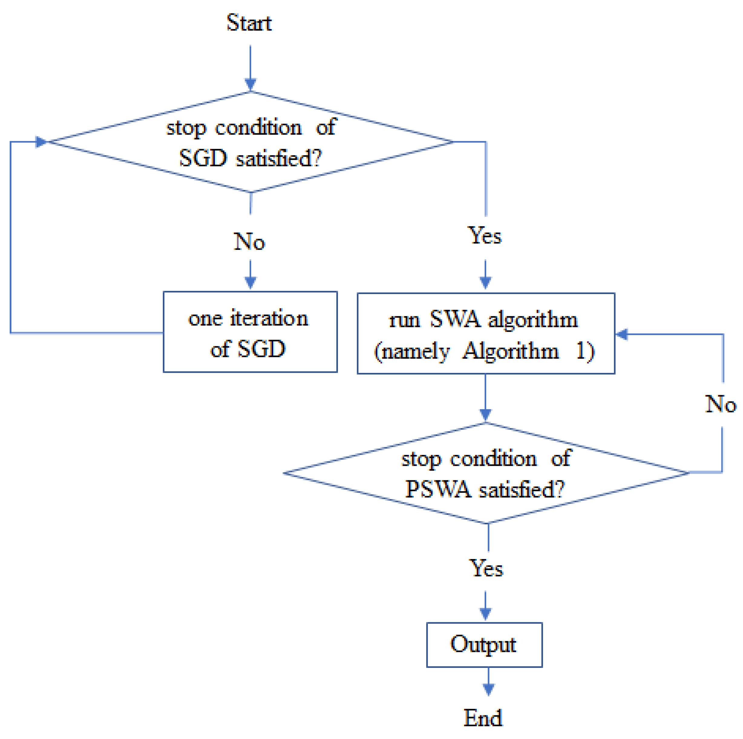
To answer the question in the title of this section, we conducted ablation studies on different DNN models and datasets. As mentioned previously, the SWA procedure consist of a re-started SGD process that uses a CHC learning-rate schedule. Using this process, a set of NN weights are sampled, and a weight-averaging operation is performed to yield the average of these sampled weights. We refer to the sampled weights as SWA samples, hereafter. The momentum and weight decaying operations were not included here to simplify the investigation.
First, we considered image classification with DNN structures, such as VGG16 [31], preactivation ResNet-164 (PreResNet-164) [32], and WideResNet-28-10 [33], using dataset CIFAR-{10,100}. For each model, SWA started after a previous converged SGD process. The results are presented in Figure 1. The effect of the weight-averaging was determined by comparing the test accuracy value of SWA to those of separate SWA samples. As was shown, neither using the CHC learning-rate schedule nor performing weight-averaging resulted in a significant increase in test accuracy. This result coincides with that revealed in the previous subsection.
We then considered cases in which the backbone SGD that ran before SWA had converged to a bad optimum, corresponding to Case II in Appendix A.1.2. In this case, we did not provide a sufficient budget for DNN training. The number of training epochs was only 30. The results based on CIFAR-{10,100} are presented in Figure 2. In this case, it is shown that the application of the CHC learning-rate schedule results in a significantly improved test accuracy by comparing test accuracy values of the SWA samples to that of the backbone SGD that ran before SWA. We also found that weight-averaging increased the test accuracy by comparing the test accuracy value of SWA to those of SWA samples.
Finally, we conducted an ablation study based on the ImageNet dataset. The results are shown in Appendix A.2. It was found that the SWA samples provided a greater increase in test accuracy values than the SGD; except for VGG16, the weight-averaging operation also increased the test accuracy.
In all aforementioned cases, the weight-averaging operation consistently provided a test accuracy value that was larger than the smallest test accuracy value provided by the separate SWA samples. It indicated that the weight-averaging operation in SWA functions similarly to tail-averaging [1], namely it decreased the variance of the test accuracy values associated with the SWA samples.

4. Periodic SWA

4.1. On the Global Geometric Structure of the DNN Loss Landscape

As presented previously, we found cases in which SWA was initialized by an SGD that did not converge well, and SWA performed notably better than its backbone SGD. However, if the preceding SGD converged well, then the performance gap between SWA and its backbone SGD was reduced or even indistinguishable. As previously shown, when the preceding SGD converged well, the NN weights employed by SWA centered around a local optimum discovered by its backbone SGD. Since those NN weights were all close to this local optimum, they were close among each other. Therefore, based on these weights, the SWA operation could only employ a highly local geometric structure around the local optimum. On the contrary, when the preceding SGD did not converge well, corresponding to a larger product of the learning rate and the stochastic gradient, the NN weight samples fed into SWA were not close to each other, so they spanned a much wider area. This motivated us to form the following hypothesis:
Is there any global geometric structure in the DNN loss landscape that could be encountered by an SGD during an early stage of its life cycle? If such a global structure exists, could it be exploited to facilitate the discovery of higher-quality local optima?
We proposed a novel algorithm design, termed a periodic SWA (PSWA), that initialized SWA during an early stage of an SGD procedure. The PSWA exploited the aforementioned possible global structures via performing weight-averaging sequentially. We describe the experimental results in the following section, which demonstrated that the PSWA outperformed its backbone SWA remarkably, thus providing evidence for the existence of such global geometric structures.
The PSWA consisted of a series of SWA procedures that processed sequentially. The first SWA procedure was initialized by an NN weight provided by the backbone SGD that processed before SWA. For each of the other SWA procedures, its starting weight seed was the output of its previous SWA procedure. As opposed to the original SWA method, which was invoked when its previous SGD converged, the PSWA was initialized when its preceding SGD was in an early stage of its operation.
A flowchart of PSWA is shown in Figure 3. Two special examples of PSWA, termed double SWA (DSWA) and triple SWA (TSWA), which consisted of two and three sequentially performed SWA procedures, are shown in Algorithm 2 and Algorithm 3, respectively. In addition, PSWA used a learning-rate schedule that was identical to its backbone SGD, as shown in Figure A1. If the sequentially performed SWA procedures could continually increase performance, as compared to the backbone SGD, then this would indicate that PSWA employed certain global structures of the loss landscape to search for the local optima.
Algorithm 2 Double Stochastic Weight Averaging (DSWA)
Input: weights w ^ , learning-rate schedule, cycle length c, number of iterations n (assumed to be multiples of 2)
Output: w dswa
1:
Run the SWA procedure (namely Algorithm 1) with input w ^ , c, n / 2 . Denote the output to be w swa .
2:
w ^ w swa .
3:
Run the SWA procedure again with input w ^ , c, n / 2 . Denote the output to be w dswa .
4:
return w dswa
Algorithm 3 Triple Stochastic Weight Averaging (TSWA)
Input: weights w ^ , learning-rate schedule, cycle length c, number of iterations n (assumed to be multiples of 3)
Output: w tswa
1:
Run the SWA procedure (namely Algorithm 1) with input w ^ , c, n / 3 . Denote the output to be w swa .
2:
w ^ w swa .
3:
Run the SWA procedure again with input w ^ , c, n / 3 . Denote the output to be w dswa .
4:
w ^ w dswa .
5:
Run the SWA procedure again with input w ^ , c, n / 3 . Denote the output to be w tswa .
6:
return w tswa

4.2. On the Performance of PSWA

The PSWA algorithm was a byproduct of our experimental findings in Section 3. The aim of our experiments was to test whether our hypothesis in Section 4.1 could be confirmed. We compared PSWA with the backbone SGD on datasets CIFAR-10 and CIFAR-100, based on DNN architectures VGG16, PreResNet-164, and WideResNet-28-10. The codes for reproducing the experimental results are available at https://github.com/ZJLAB-AMMI/PSWA (accessed on 22 February 2023). The momentum factor for the SGD was 0.9, and the weight-decay parameter was 0.0005. The PSWA initialized after the 40th epoch with a period of 20 epochs. Within one period of the PSWA, a full SWA procedure was conducted. In a SWA procedure, we sampled one NN weight per epoch and then averaged the weights that had been sampled within this SWA procedure, as the current output of PSWA.
The experimental results are shown in Figure 4. We found that PSWA provided a remarkable performance gain, as compared to its backbone SGD, during the early stage of the training process. We also conducted an experiment in which we compared SWA with DSWA and TSWA, and we conducted the same number of iterations to guarantee that their computational budgets were approximately the same. We did not use the momentum and weight decay methods to prevent their influences on the comparison.
We found that if the backbone SGD that ran before SWA did not converge or converged to a bad local optimum, corresponding to Case II in Appendix A.1.2, DSWA and TSWA found flatter optima that led to a better generalization than SWA, as shown in Table 4 and Table 5, and Figure 5. If the backbone SGD converged well, corresponding to Case I in Appendix A.1.2, then DSWA and TSWA failed to find flatter optima than SWA, as shown in Figure 6. Note that Figure 5 and Figure 6 were obtained using the same procedures as those used to obtain Figure 5 in [5].

4.3. Discussions

The previous results on PSWA showed experimental evidence for the existence of global geometric structures in the DNN loss landscape that could be perceived by an SGD algorithm agent at an early stage of its operation and demonstrated that such structures could be exploited by the weight-averaging operations for improving the backbone SGD. From an algorithmic perspective, we could not claim that PSWA was better than SGD, since the quality of their final results at the end of the training process were indistinguishable. If the training budget could not support the whole training process, then PSWA was clearly preferable to an SGD, since it provided better weight samples than an SGD during an early stage of the training process. Our experimental results using DSWA and TSWA provided a geometric insight that the weight-averaging operation could occasionally lead to wider optima. Specifically, when the momentum and weight-decaying techniques were not used and the preceding SGD converged well, the weight-averaging operation failed to find wider optima. This result was consistent with that reported in Section 3.1.

5. Conclusions

In this paper, we investigated the contributions of the weight-averaging operation and the cyclical or high-constant learning-rate scheduling to the SWA process. Through experiments on a broad range of NN architectures, we identified a link between SGD and the global loss landscape and developed a novel insight from statistical and geometric perspectives regarding SWA. Specifically, we found that SWA was useful because it provided a mechanism to combine the advantages of the weight-averaging operation and the CHC learning-rate schedule. The CHC learning-rate schedule discovered global-scale geometric structures, and weight-averaging exploited such structures. By leveraging SGD’s behavior in its early training phase, we proposed a novel algorithm, periodic SWA, which proved to be capable of finding high-quality local optima more quickly than SGD.
Although we covered a broad range of network architectures and different types of datasets in our experiments, our findings still lacked theoretical support and may not be applicable for all DNN tasks. However, our work may promote more theoretical and algorithmic research on demonstrating, discovering, and exploiting non-local geometric structures of DNN’s loss landscape in the future.

Author Contributions

Conceptualization, B.L.; methodology, B.L.; software, H.G., J.J. and B.L.; validation, H.G. and B.L.; formal analysis, B.L.; investigation, B.L.; resources, B.L.; data curation, H.G. and J.J.; writing—original draft preparation, B.L.; writing—review and editing, B.L.; visualization, H.G., J.J. and B.L.; supervision, B.L.; project administration, B.L.; funding acquisition, B.L. All authors have read and agreed to the published version of the manuscript.

Funding

This research was funded by Research Initiation Project of Zhejiang Lab grant number 2021KB0PI01 and Exploratory Research Project of Zhejiang Lab grant number 2022RC0AN02.

Institutional Review Board Statement

Not applicable.

Informed Consent Statement

Not applicable.

Data Availability Statement

All datasets used in this study are publicly open-sourced. We provided links to these datasets in the maintext.

Conflicts of Interest

The authors declare no conflict of interest.

Appendix A. Experimental Settings and More Experimental Results

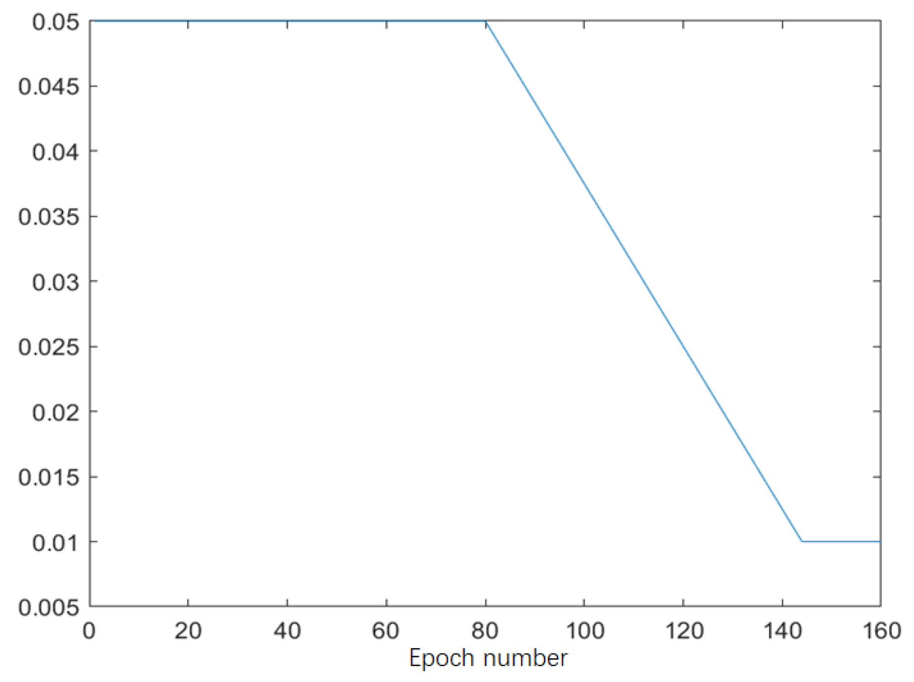
Appendix A.1. Experimental Setting

In this section, we describe our experimental design, corresponding to the results presented in Section 3 and Section 4.

Appendix A.1.1. Experimental Settings for Results Reported in Section 3.1

For the graph-classification task, we conducted our experiments on a public open-source dataset MUTAG, which has commonly been used for graph-classification tasks. See details about this dataset at https://paperswithcode.com/dataset/mutag (accessed on 1 November 2021).We used Adam [34] to train a GIN model for 300 epochs. We set the learning rate α at 0.01 and used the default parameter setting for the exponential decay rates β 1 and β 2 , namely let β 1 = 0.9 and β 2 = 0.999 , respectively. For SWA, it initialized at the 270th epoch, using a constant learning rate of 0.02.
For experiments on the text dataset MRPC (see details about this dataset at https://paperswithcode.com/dataset/mrpc (accessed on 1 November 2021)) the learning rate of SGD was fixed at 10 4 during the first 20 epochs; then, it was linearly decreased to 10 6 in the following 20 epochs and then was fixed at 10 6 for the last 10 epochs. The momentum and the weight-decaying factors were set at 0.9 and 0.01, respectively. SWA was initialized at the 45th epoch. For each epoch of SWA, the learning rate was linearly decreased from 5 × 10 5 to 5 × 10 6 .

Appendix A.1.2. Experimental Settings for Results Reported in Section 3.2

For the image-classification experiments presented in Section 3.2, we considered two main cases, termed Case I and Case II, for each DNN architecture under consideration. In Case I, we processed SWA after a converged SGD. In Case II, we processed it after a non-converged SGD. We adopted the same type of learning-rate schedule as used in [5]. An example of learning-rate schedule we used is shown in Figure A1. This learning-rate schedule covered L = 160 epochs in total. The first half-segment of this learning-rate schedule had a constant higher value C h , followed by a segment of the learning-rate schedule that consisted of linearly decreased learning-rate values. The ending segment of this learning-rate schedule had a constant lower value C l . The learning-rate schedule is shown in Figure A1, C h = 0.05 , and C l = 0.01 . For Case I, we set the value of L to be sufficiently high and that of C l sufficiently low to guarantee that the SGD process that processed before SWA converged. For Case II, we set a low value, such as 30, for L to ensure that the SGD that processed before SWA did not converge. For the SWA procedure, the cycle length c had a value that ensured a cycle was equal to an epoch. We adopted the same CHC learning-rate schedule used in [5] for the SWA procedure. The mini-batch size was set at 128 for all experiments.
Figure A1. An example of the learning-rate schedules used in our experiments.
Applsci 13 02935 g0a1

Appendix A.2. Experiment on ImageNet

We conduct the same ablation study in Section 3.2 on the ImageNet dataset. We processed SWA based on the backbone DNN models VGG16, ResNet-50, ResNet-152, and DenseNet-161, which were contained in PyTorch. The results are presented in Figure A2.
Figure A2. Ablation study using the ImageNet dataset. The legends are defined in the same way as in Figure 1. The top left, top right, bottom left, and bottom right panels show results corresponding to VGG16, ResNet-50, ResNet-152, and DenseNet-161, respectively. Note that SWA began based on the pre-trained models in Pytorch. Therefore, the horizontal axis label initialized with epoch 1.
Applsci 13 02935 g0a2

Appendix A.3. Experiments with a Toy CNN Model

In this experiment, we removed the momentum module from the SGD. We trained a toy CNN model on CIFAR-10 and received an over-fitted result, as shown in Figure A3. We recorded the weight value at the end of each epoch and calculated the corresponding test accuracy value. The maximum test accuracy value of 0.683 appeared at the 45th epoch. The test accuracy corresponding to the last iterate of SGD was 0.680. We replaced the last L = 5 iterations of the SGD with the SWA procedure, resulting in a test accuracy value of w swa = 0.679 . We changed the value of L to 20 and obtained w swa = 0.680 . This indicated that SWA did not lead to wider optima in this case.
A similar phenomenon occurred when we replaced the toy CNN model with PreResNet-164. We used the open-source code by [5], while removing influences of the momentum and the L2-based weight regularization, on SWA. As is shown in Figure A4, the SGD converged after the 120th epoch at a test accuracy of 89.24%. We processed SWA after the 140th epoch and obtained a test accuracy of 89.17%, which was smaller than the test accuracy achieved by the converged SGD.
Figure A3. The over-fitted result obtained when training a toy CNN model on CIFAR-10. This CNN had 9 layers: the input layer, the convolution layer, a max-pooling layer, another convolution layer, another max-pooling layer, the flatten layer, 2 fully connected layers, and a softmax layer.
Applsci 13 02935 g0a3
Figure A4. Training PreResNet-164 on CIFAR-10.
Applsci 13 02935 g0a4

Appendix A.4. Experiments with Graph Data

We showed experimental settings associated with the graph data experiments presented in Section 3.1 in Table A1, Table A2, Table A3 and Table A4.
Table A1. The parameter settings for the GNN experiments. The baseline optimizer was Adam with a weight-decay factor of 0.0005. The variable L denotes the total number of epochs, α is the learning rate of the Adam optimizer, α SWA is the constant learning rate used by SWA, and t SWA is the starting point to launch SWA.
ParameterGCNGraphSAGEGAT
L20020300
α 0.010.0030.005
t SWA 18015270
α SWA 0.020.010.01
Table A2. The parameter settings for the graph-classification task on dataset NCI1. The baseline optimizer was Adam with weight-decay factor of 0.0005. The variable L denotes the total number of epochs, α is the learning rate of the Adam optimizer, α SWA is the constant learning rate used by SWA, and t SWA is the starting point to launch SWA.
ParameterMinCutPoolSAGPool
L1000300
α 0.0010.003
t SWA 900270
α SWA 0.010.01
Table A3. The parameter settings for the graph-classification task on dataset D&D. The baseline optimizer was Adam with weight-decay factor of 0.0005. The variable L denotes the total number of epochs, α is the learning rate of the Adam optimizer, α SWA is the constant learning rate used by SWA, and t SWA is the starting point to launch SWA.
ParameterMinCutPoolSAGPool
L50150
α 0.0010.003
t SWA 35120
α SWA 0.010.005
Table A4. The parameter settings for the graph-classification task on dataset PROTEINS. The baseline optimizer was Adam with weight-decay factor of 0.0005. The variable L denotes the total number of epochs, α is the learning rate of the Adam optimizer, α SWA is the constant learning rate used by SWA, and t SWA is the starting point to launch SWA.
ParameterMinCutPoolSAGPool
L500300
α 0.00010.003
t SWA 450270
α SWA 0.0010.01

References

  1. Jain, P.; Kakade, S.; Kidambi, R.; Netrapalli, P.; Sidford, A. Parallelizing stochastic gradient descent for least squares regression: Mini-batching, averaging, and model misspecification. J. Mach. Learn. Res. 2018, 18, 1–42. [Google Scholar]
  2. Ruppert, D. Efficient Estimations from a Slowly Convergent Robbins-Monro Process; Technical Report; Cornell University Operations Research and Industrial Engineering: New York, NY, USA, 1988. [Google Scholar]
  3. Polyak, B.T.; Juditsky, A.B. Acceleration of stochastic approximation by averaging. SIAM J. Control Optim. 1992, 30, 838–855. [Google Scholar] [CrossRef] [Green Version]
  4. Neu, G.; Rosasco, L. Iterate averaging as regularization for stochastic gradient descent. In Proceedings of the Conference on Learning Theory, Stockholm, Sweden, 6–9 July 2018; pp. 3222–3242. [Google Scholar]
  5. Izmailov, P.; Podoprikhin, D.; Garipov, T.; Vetrov, D.; Wilson, A.G. Averaging weights leads to wider optima and better generalization. In Proceedings of the Conference on Uncertainty in Artificial Intelligence (UAI), Monterey, CA, USA, 6–10 August 2018; pp. 1–10. [Google Scholar]
  6. Cha, J.; Chun, S.; Lee, K.; Cho, H.C.; Park, S.; Lee, Y.; Park, S. SWAD: Domain generalization by seeking flat minima. In Proceedings of the Thirty-fifth Conference on Neural Information Processing Systems, Virtual, 6–14 December 2021. [Google Scholar]
  7. Hwang, J.W.; Lee, Y.; Oh, S.; Bae, Y. Adversarial Training with Stochastic Weight Average. In Proceedings of the IEEE International Conference on Image Processing (ICIP), Anchorage, AK, USA, 19–22 September 2021; pp. 814–818. [Google Scholar]
  8. Keskar, N.S.; Mudigere, D.; Nocedal, J.; Smelyanskiy, M.; Tang, P.T.P. On large-batch training for deep learning: Generalization gap and sharp minima. In Proceedings of the International Conference on Learning Representations, Toulon, France, 24–26 April 2017. [Google Scholar]
  9. Smith, L.N. Cyclical learning rates for training neural networks. In Proceedings of the IEEE Winter Conference on Applications of Computer Vision (WACV), Santa Rosa, CA, USA, 24–31 March 2017; pp. 464–472. [Google Scholar]
  10. Loshchilov, I.; Hutter, F. SGDR: Stochastic gradient descent with warm restarts. In Proceedings of the International Conference on Learning Representations, Toulon, France, 24–26 April 2017. [Google Scholar]
  11. Garipov, T.; Izmailov, P.; Podoprikhin, D.; Vetrov, D.; Wilson, A.G. Loss surfaces, mode connectivity, and fast ensembling of dnns. In Proceedings of the 32nd International Conference on Neural Information Processing Systems, Montréal, QC, Canada, 3–8 December 2018; pp. 8803–8812. [Google Scholar]
  12. Huang, G.; Li, Y.; Pleiss, G.; Liu, Z.; Hopcroft, J.E.; Weinberger, K.Q. Snapshot ensembles: Train 1, get M for free. In Proceedings of the International Conference on Learning Representations, Toulon, France, 24–26 April 2017. [Google Scholar]
  13. Smith, L.N.; Topin, N. Super-convergence: Very fast training of neural networks using large learning rates. In Proceedings of the Artificial Intelligence and Machine Learning for Multi-Domain Operations Applications, Baltimore, MD, USA, 14–18 April 2019; International Society for Optics and Photonics, SPIE: Bellingham, WA, USA, 2019; Volume 11006, p. 1100612. [Google Scholar]
  14. Smith, L.N.; Topin, N. Exploring loss function topology with cyclical learning rates. arXiv 2017, arXiv:1702.04283. [Google Scholar]
  15. Ghorbani, B.; Krishnan, S.; Xiao, Y. An investigation into neural net optimization via hessian eigenvalue density. In Proceedings of the International Conference on Machine Learning, Long Beach, CA, USA, 9–15 June 2019; pp. 2232–2241. [Google Scholar]
  16. Sagun, L.; Evci, U.; Guney, V.U.; Dauphin, Y.; Bottou, L. Empirical analysis of the hessian of over-parametrized neural networks. arXiv 2017, arXiv:1706.04454. [Google Scholar]
  17. Yao, Z.; Gholami, A.; Keutzer, K.; Mahoney, M.W. Pyhessian: Neural networks through the lens of the hessian. In Proceedings of the IEEE International Conference on Big Data (Big Data), Atlanta, GA, USA, 10–13 December 2020; pp. 581–590. [Google Scholar]
  18. Yang, Y.; Hodgkinson, L.; Theisen, R.; Zou, J.; Gonzalez, J.E.; Ramchandran, K.; Mahoney, M.W. Taxonomizing local versus global structure in neural network loss landscapes. In Proceedings of the Thirty-fifth Conference on Neural Information Processing Systems, Virtual, 6–14 December 2021; Volume 34. [Google Scholar]
  19. Kleiner, A.; Neyshabur, B.; Mobahi, H.; Foret, P. Sharpness-aware Minimization for Efficiently Improving Generalization. In Proceedings of the International Conference on Learning Representations, Virtual Event, Austria, 3–7 May 2021. [Google Scholar]
  20. Allen-Zhu, Z.; Li, Y.; Song, Z. A convergence theory for deep learning via over-parameterization. In Proceedings of the International Conference on Machine Learning, Long Beach, CA, USA, 9–15 June 2019; pp. 242–252. [Google Scholar]
  21. Cheridito, P.; Jentzen, A.; Rossmannek, F. Non-convergence of stochastic gradient descent in the training of deep neural networks. J. Complex. 2021, 64, 101540. [Google Scholar] [CrossRef]
  22. Krizhevsky, A.; Hinton, G. Learning Multiple Layers of Features from Tiny Images; Technical Report; University of Toronto: Toronto, ON, Canada, 2009. [Google Scholar]
  23. Deng, J.; Dong, W.; Socher, R.; Li, L.; Li, K.; Fei-Fei, L. ImageNet: A large-scale hierarchical image database. In Proceedings of the IEEE Conference on Computer Vision and Pattern Recognition, Miami, FL, USA, 20–25 June 2009; pp. 248–255. [Google Scholar]
  24. Russakovsky, O.; Deng, J.; Su, H.; Krause, J.; Satheesh, S.; Ma, S.; Huang, Z.; Karpathy, A.; Khosla, A.; Bernstein, M.; et al. ImageNet large scale visual recognition challenge. Int. J. Comput. Vis. 2015, 115, 211–252. [Google Scholar] [CrossRef] [Green Version]
  25. Yao, L.; Mao, C.; Luo, Y. Graph convolutional networks for text classification. In Proceedings of the AAAI Conference on Artificial Intelligence, Honolulu, HI, USA, 27 January–1 February 2019; pp. 7370–7377. [Google Scholar]
  26. Hamilton, W.; Ying, Z.; Leskovec, J. Inductive representation learning on large graphs. In Proceedings of the 2017 Conference on Neural Information Processing Systems, Long Beach, CA, USA, 4–9 December 2017; Volume 30. [Google Scholar]
  27. Veličković, P.; Cucurull, G.; Casanova, A.; Romero, A.; Lio, P.; Bengio, Y. Graph attention networks. arXiv 2017, arXiv:1710.10903. [Google Scholar]
  28. Bianchi, F.M.; Grattarola, D.; Alippi, C. Spectral clustering with graph neural networks for graph pooling. In Proceedings of the International Conference on Machine Learning, Virtual Event, 13–18 July 2020; pp. 874–883. [Google Scholar]
  29. Lee, J.; Lee, I.; Kang, J. Self-attention graph pooling. In Proceedings of the International Conference on Machine Learning, Long Beach, CA, USA, 9–15 June 2019; pp. 3734–3743. [Google Scholar]
  30. Kaddour, J.; Liu, L.; Silva, R.; Kusner, M.J. When Do Flat Minima Optimizers Work? arXiv 2022, arXiv:2202.00661. [Google Scholar]
  31. Simonyan, K.; Zisserman, A. Very deep convolutional networks for large-scale image recognition. In Proceedings of the International Conference on Learning Representations, San Diego, CA, USA, 7–9 May 2015. [Google Scholar]
  32. He, K.; Zhang, X.; Ren, S.; Sun, J. Identity mappings in deep residual networks. In Proceedings of the European Conference on Computer Vision (ECCV), Amsterdam, The Netherlands, 11–14 October 2016; pp. 630–645. [Google Scholar]
  33. Zagoruyko, S.; Komodakis, N. Wide residual networks. arXiv 2016, arXiv:1605.07146. [Google Scholar]
  34. Kingma, D.P.; Ba, J. Adam: A method for stochastic optimization. arXiv 2014, arXiv:1412.6980. [Google Scholar]
Figure 1. Ablation study of the CHC learning-rate schedule and the weight-averaging operation for DNNs that converge well. The legend “SGD" denotes the test accuracy value associated with the NN weight as provided by the backbone SGD at the time point when SWA was started. The legend “SWA samples” denotes test accuracy values associated with NN weights sampled during the SWA procedure. The legend “SWA” denotes the test accuracy value associated with the mean of NN weights sampled during the SWA procedure. The sub-figures in the left/middle/right columns correspond to VGG16/PreResNet-164/WideResNet-28-10. The sub-figures in the top/bottom rows correspond to dataset CIFAR-10/100.
Applsci 13 02935 g001
Figure 2. Ablation study on the CHC learning-rate schedule and the weight-averaging operation for DNNs that did not converge well. The legends are defined in the same way as in Figure 1. The sub-figures in the left/middle/right columns correspond to VGG16/PreResNet-164/WideResNet-28-10. The sub-figures in the top/bottom rows correspond to dataset CIFAR-10/CIFAR-100.
Applsci 13 02935 g002
Figure 3. Block schema of PSWA. PSWA consisted of a backbone SGD that processed before the SWA operations and a series of SWA procedures that processed sequentially. The first SWA procedure was initialized by the output of the backbone SGD. For each of the other SWA procedures, its starting weight seed was the output of its previous SWA procedure. In contrast to the original SWA method, which was invoked when its preceding SGD converged, the PSWA was initialized when its preceding SGD was in an early stage of its operation.
Applsci 13 02935 g003
Figure 4. Test accuracy comparison between PSWA and its backbone SGD. The sub-figures in the left/middle/right columns correspond to VGG16/PreResNet-164/WideResNet-28-10, respectively. The sub-figures in the top/bottom rows correspond to dataset CIFAR-10/CIFAR-100, respectively.
Applsci 13 02935 g004
Figure 5. Cross-entropy training loss and testing error as a function of a point on the line connecting the SWA and DSWA (or TSWA) solutions on CIFAR-100. DSWA and TSWA were initialized by a non-converged preceding SGD procedure. Left: PreResNet-164. Right: VGG16.
Applsci 13 02935 g005
Figure 6. Cross-entropy training loss and testing error as a function of a point on the line connecting the SWA and DSWA (or TSWA) solutions on CIFAR-10. DSWA and TSWA were initialized by a converged preceding SGD procedure. Left: PreResNet-164. Right: VGG16.
Applsci 13 02935 g006
Table 1. A summary of advantages and disadvantages of related works on IA (iterates averaging), CLR (cyclical learning rates), ensemble, and LL (loss landscape), and this work. We reviewed whether they provided statistical or geometric insights and practical algorithms.
Statistical InsightGeometric InsightAlgorithm
IA×
CLR [9,10]××
Ensemble [11,12,13,14]×
LL [6,8,15,16,17,18,19]×
this work
Table 2. Test accuracy (%) comparison between Adam and SWA for the graph-node-classification task on datasets Cora, Citeseer, and Pubmed. Best results are bolded.
CoraCiteseerPubmed
AdamSWAAdamSWAAdamSWA
GCN81.2 ± 0.47 81.3 ± 0.21 70.5 ± 0.45 70.8 ± 0.41 79.5 ± 0.29 79.6 ± 0.26
GraphSAGE80.2 ± 0.22 79.3 ± 0.49 69.8 ± 0.54 69.7 ± 0.16 77.8 ± 0.17 77.7 ± 0.29
GAT81.6 ± 0.43 81.7 ± 0.52 70.6 ± 0.26 70.4 ± 0.25 76.1 ± 0.43 76.2 ± 0.28
Table 3. Test accuracy (%) comparison between Adam and SWA for the graph-classification task on datasets NCI1, D&D, and PROTEINS. Best results are bolded.
NCI1D&DPROTEINS
AdamSWAAdamSWAAdamSWA
MinCutPool74.78 ± 0.42 75.25 ± 0.14 79.67 ± 0.69 80.86 ± 0.85 76.44 ± 1.50 77.34 ± 1.83
SAGPool71.63 ± 0.88 72.57 ± 0.49 71.89 ± 0.33 70.87 ± 0.45 77.73 ± 1.16 78.37 ± 1.10
Table 4. Test accuracy (%) comparison among SGD, SWA, and DSWA on CIFAR-10, based on a toy CNN model. The preceding SGD procedure did not converge. The best results are bolded.
SGDSWADSWA
57.10 ± 0.48 67.27 ± 0.29 69.49 ± 0.33
Table 5. Test accuracy (%) comparison among SGD, SWA, DSWA, and TSWA on CIFAR-100. The SGD procedure that processed before SWA does not converge. Best results are bolded.
VGG16PreResNet-164WideResNet-28-10
SGD55.28 ± 0.62 70.55 ± 0.84 76.30 ± 0.81
SWA65.89 ± 0.24 76.45 ± 0.63 80.95 ± 0.27
DSWA68.44 ± 0.25 77.26 ± 0.49 81.18 ± 0.14
TSWA68.68 ± 0.16 77.33 ± 0.45 81.11 ± 0.12
Disclaimer/Publisher’s Note: The statements, opinions and data contained in all publications are solely those of the individual author(s) and contributor(s) and not of MDPI and/or the editor(s). MDPI and/or the editor(s) disclaim responsibility for any injury to people or property resulting from any ideas, methods, instructions or products referred to in the content.

