Article

A Lightweight Robust Distance Estimation Method for Navigation Aiding in Unsupervised Environment Using Monocular Camera

1
Faculty of Applied Sciences, Macao Polytechnic University, Macao SAR 999078, China
2
Department of Computer Science and Engineering, University of Bologna, 40126 Bologna, Italy
3
Autonomous Robotics Research Center, Technology Innovation Institute (TII), Abu Dhabi P.O. Box 9639, United Arab Emirates
4
Samueli Computer Science Department, University of California, Los Angeles, CA 90095, USA
*
Author to whom correspondence should be addressed.
Appl. Sci. 2023, 13(19), 11038; https://doi.org/10.3390/app131911038
Submission received: 9 September 2023 / Revised: 28 September 2023 / Accepted: 3 October 2023 / Published: 7 October 2023
(This article belongs to the Special Issue Modern Computer Vision and Pattern Recognition)

Abstract

:
This research addresses the challenges of visually impaired individuals’ independent travel by avoiding obstacles. The study proposes a distance estimation method for uncontrolled three-dimensional environments to aid navigation towards labeled target objects. Utilizing a monocular camera, the method captures cuboid objects (e.g., fences, pillars) for near-front distance estimation. A Field of View (FOV) model calculates the camera’s angle and arbitrary pitch relative to the target Point of Interest (POI) within the image. Experimental results demonstrate the method’s proficiency in detecting distances between objects and the source camera, employing the FOV and Point of View (POV) principles. The approach achieves a mean absolute percentage error (MAPE) of 6.18% and 6.24% on YOLOv4-tiny and YOLOv4, respectively, within 10 m. The distance model only contributes a maximum error of 4% due to POV simplification, affected by target object characteristics, height, and selected POV. The proposed distance estimation method shows promise in drone racing navigation, EV autopilot, and aiding visually impaired individuals. It offers valuable insights into dynamic 3D environment distance estimation, advancing computer vision and autonomous systems.

1. Introduction

Visual impairment (VI) is a significant public health concern that affects people of all ages and is caused by a range of factors, including age-related eye diseases, genetic disorders, injuries, and infections [1]. The global population of individuals suffering from VI, including those who are completely blind, moderately visually impaired, and severely visually impaired, has reached more than 300 million [2]. The increasing number of visual impairment (VI) cases highlights the critical need to improve accessibility and mobility for visually impaired individuals, who face significant challenges in navigating public spaces due to the low success rate of obstacle avoidance.
Therefore, governments of different countries are attempting to design various assistive living facilities for individuals with visual impairments. In the United States, guide dogs and white canes remain essential tools. In addition, the emergence of advanced technologies has also enhanced the independent mobility of individuals with visual impairments and blindness. GPS-based navigation systems, such as smartphone applications and standalone devices, provide step-by-step navigation and information about points of interest. Furthermore, obstacle detection devices and electronic travel aids, such as ultrasonic canes and wearable sensors, assist individuals in navigating their surroundings [3]. In the United Kingdom, tactile pavements and signage have been implemented in public spaces to improve accessibility and orientation [4]. The “Haptic Radar” system in Japan utilizes vibrations to provide real-time feedback on surrounding objects [5].
However, the accessibility of these facilities is often inadequate in older districts, leading to the use of personal navigation tools such as white canes and guide dogs [6]. While white canes are a popular option, their short range and potential interference with other pedestrians may hinder mobility in crowded spaces. Alternatively, guide dogs offer effective guidance, but their high cost and restrictions on public transportation may limit their widespread use [7]. For the existing advanced technologies, engineers and manufacturers face technical challenges in ensuring the accuracy and reliability of navigation and object detection systems [3]. In daily life, it is essential to prioritize efforts to address the challenges faced by visually impaired individuals, as the loss of eyesight can be a debilitating experience.
Recently, machine learning techniques have greatly improved object recognition accuracy in computer vision [8]. This has led to the development of sophisticated models that can recognize objects in complex environments. These advancements have enabled the creation of highly accurate and reliable computer vision systems for applications such as self-driving cars, medical imaging, and surveillance. Near-field object detection can also benefit from these machine-learning techniques [9], allowing for accurate real-time detection of nearby objects. To locate the fences in the street, object detection is required, and it can be accomplished by a deep learning approach [10]. The distance information can then be utilized for various applications, including robotics, drone racing, autonomous vehicles, and navigation assistance tools [11,12,13,14]. Based on the trained model on the dataset, detection of the fences from public objects by the images and videos are captured by the user camera. Detected objects and their categories are remarked on in the corresponding media content. After eliminating duplicated and low-confident detection, the result is then passed to the distance estimation process.
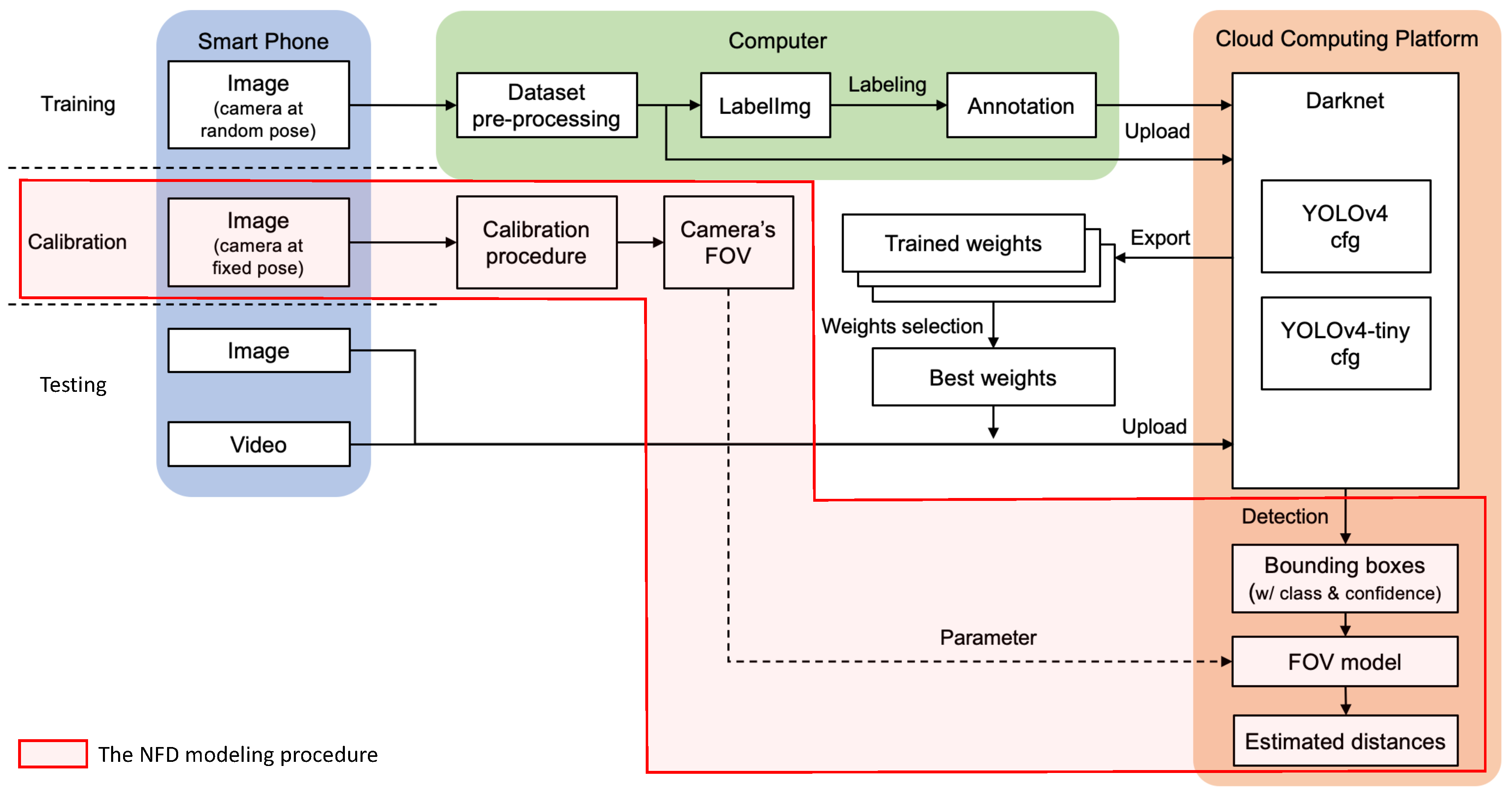
In this article, machine learning is applied to obstacle detection of near distance in front, allowing visually impaired people to walk freely and safely. The objective of this work is to develop a new approach to navigation aid that assists visually impaired people to travel independently with confidence. A solution, Near Front Distance (NFD) for estimating near-front distance using a monocular camera on public objects based on a deep learning approach is proposed, which consists of camera calibration and distance estimation modeling. A distance estimation process is applied to the images taken by the camera on intrinsic parameters after calibration. The position of detected objects on images are converted from the image coordinates to the actual coordinates based on the position or size information and within assumptions. Our distance estimation model can combine deep-learning-based object detection methods to accurately measure the distance between objects and the camera inside the field of view. Ultimately, our work contributes to bridging the gap between computer vision advancements and practical applications, particularly in scenarios where the accurate measurement of distances to obstacles is crucial.
We utilized a published dataset on public objects in the uncontrolled environment, which was specifically designed for navigation-aiding purposes [15]. The primary contributions of this work can be summarized as follows:
  • Development of a novel integration algorithm that utilizes image data from a monocular camera and the camera’s pose to estimate the distance to target objects effectively. The algorithm calculates the object’s distance on the front by the pixel on the picture after YOLOv4 detection.
  • Evaluation of the performance of deep learning models when applied to the novel algorithm for distance estimation.
The remainder of the work is divided into the following sections: The related works are comprehensively addressed in Section 2. In Section 3, the methodology used in this study is described in detail, including the approach for measuring distance from various positions and points of interest. The results of the suggested approach are shown in Section 4, which also presents the empirical findings. Finally, in Section 5, we offer a comprehensive summary of the study, highlighting the main conclusions, and provide some closing thoughts.

2. Related Works

In this section, conventional and deep learning approaches are investigated for depth estimation. In order to understand the conditions of the surroundings and the distances to the targets or obstacles, sensors such as cameras, radar, and LiDAR are commonly used.

2.1. Sensors for Distance Measurement

The camera is a widely used and cost-effective sensor for environmental perception. It mimics the capabilities of the human visual system, excelling in the recognition of shapes and colors of objects. However, it does have limitations, particularly in adverse weather conditions with reduced visibility.
The radar (radio detection and ranging) is widely used to precisely track the distance, angle, or velocity of objects. Radars can be broken down into a transmitter and receiver. The transmitter sends radio waves in the targeted direction and the waves are reflected when they reach a significant object. The receiver picks up the reflected waves and gives information about the object’s location and speed. The greatest advantage of the radar is that it is not affected by visibility, lighting, and noise in the environment. However, compared to a camera, a radar is low-definition modeling and is weak at providing the precise shape of objects and identifying what the object is.
The mechanism of the LiDAR (light detection and ranging) is similar to the radar but utilize laser light to determine ranges instead of radio wave. The LiDAR is a more advanced version of a radar that can provide extremely low error distance measurement. It is also capable of measuring thousands of points at the same time to model up a precise 3D depiction of an object or surrounding environment [16]. The disadvantages of the LiDAR are its high cost and the requirement of a remarkable amount of computing resources compared to cameras and radars.
Although the costs of cameras, radar systems, and LiDAR can vary significantly due to factors such as brand, specifications, and quality, a general assessment of equipment costs with comparable capabilities reveals the following: Cameras typically range in price from $100 to several thousand dollars, depending on factors such as resolution, image quality, and additional features. Radar systems used for object detection and tracking start at a few hundred dollars for basic short-range sensors, while more advanced and specialized radar systems can cost several thousand dollars or more. Likewise, LiDAR sensors range in price from a few hundred dollars for entry-level sensors to several thousand dollars for high-end models with extended range, higher resolution, and faster scanning capabilities.
Considering the pros and cons of the three types of sensors for distance measurement, the camera is the most appropriate sensor to be utilized in the research due to its low cost, being less sophisticated, and its high definition. The 2D information recognized by the camera can be adopted directly by the deep learning algorithms of object detection.

2.2. Traditional Distance Estimation

Typical photos taken from a monocular camera are shown in two dimensions that would require extra information for distance estimation. Distance estimation (also known as depth estimation) is an inverse problem [17] that tries to measure the distance between 3D objects from insufficient information provided in the 2D view.
The earliest algorithms for depth estimation were developed based on stereo vision. Researchers utilize geometry to constrain and replicate the idea of stereopsis mathematically. Scharstein and Szeliski [18] conducted a comparative evaluation of the best-performing stereo algorithms at that time. Meanwhile, Stein et al. [19] developed methods to estimate the distance from a monocular camera. They investigated the possibility of performing distance control to an accuracy level sufficient for an Adaptive Cruise Control system. A single camera is installed in a vehicle using the laws of perspective to estimate the distance based on a constrained environment: the camera is at a known height from a planar surface in the near distance and the objects of interest (the other vehicles) lie on that plane. A radar is equipped for obtaining the ground truth. The results show that both distance and relative velocity can be estimated from a single camera and the actual error lies mostly within the theoretical bounds. Park et al. [20] also proposed a distance estimation method for vision-based forward collision warning systems with a monocular camera. The system estimates the virtual horizon from information on the size and position of vehicles in the image, which is obtained by an object detection algorithm and calculates the distance from vehicle position in the image with the virtual horizon even when the road inclination varies continuously or lane markings are not seen. To enable the distance estimation in vehicles, Tram and Yoo [21] also proposed a system to determine the distance between two vehicles using two low-resolution cameras and one of the vehicle’s rear LED lights. Since the poses of the two cameras are pre-determined, the distances between the LED and the cameras, as well as the vehicle-to-vehicle distance can be calculated based on the pinhole model of the camera as the focal lengths of the cameras are known. The research also proposes a resolution compensation method to reduce the estimation error by a low-resolution camera. Moreover, Chen et al. [22] proposed an integrated system that combines vehicle detection, lane detection, and vehicle distance estimation. The proposed algorithm does not require calibrating the camera or measuring the camera pose in advance as they estimate the focal length from three vanishing points and utilize lane markers with the associated 3D constraint to estimate the camera pose. The SVM with Radial Basis Function (RBF) kernel is chosen to be the classifier of vehicle detection and Canny edge detection and Hough transform are employed for the lane detection.

2.3. Depth Estimation Using Deep Learning

Nowadays, to achieve depth estimation using a monocular camera, neural networks are commonly used. Eigen et al. [23] proposed one of the typical solutions that presented a solution to measure depth relations by employing two deep network stacks: one that makes a coarse global prediction based on the entire image, and another that refines the prediction locally. By applying the raw datasets (NYU Depth and KITTI) as large sources of training data, the method matches detailed depth boundaries without the need for superpixelation.
Another solution that can overcome the weakness of using CNN for depth estimation is that vast amounts of data need to be manually labeled before training [24]. A CNN for single-view depth estimation that can be trained end-to-end, unsupervised, using data captured by a stereo camera without requiring a pre-training stage or annotated ground-truth depths. To achieve that, an inverse warp of the target image is generated using the predicted depth and known inter-view displacement to reconstruct the source image; the photometric error in the reconstruction is the reconstruction loss for the encoder. Zhou et al. [25] also presented an unsupervised learning framework for the task of monocular depth and camera motion estimation from unstructured video sequences. The system is trained on unlabeled videos and yet performs comparably with approaches that require ground-truth depth or pose for training. As a whole, Table 1 highlights the various deep-learning-based approaches to depth estimation.
While deep learning technology has showcased its proficiency in depth perception and measurement, certain challenges persist: (i) Specialized Equipment: Generating media data with depth information necessitates specialized equipment like Kinect cameras, ToF cameras, or LiDAR sensors to create training datasets. Without such equipment, the laborious task of manually labeling each object with ground truth distance becomes inevitable. (ii) Unsupervised Framework: Unsupervised monocular camera depth estimation typically relies on stereo video sequences as input. It leverages geometric disparities, photometric errors, or feature discrepancies between adjacent frames as self-supervised signals for model training.
In this study, we propose a novel integration approach for navigation that merges computer vision and deep learning in object detection and distance estimation. This approach is user-friendly, easily maintainable, and cost-effective. Importantly, it demands fewer computational resources, making it suitable for implementation on smartphones and similar devices.

3. Methodology

In this work, NFD for estimating near-front distance using a monocular camera on public objects is proposed. The solution can be utilized as a navigation aid for visually impaired people. Figure 1 depicts the architecture of NFD, which is a three-tier cloud solution that consists of a smartphone with a built-in monocular camera, a computer for image processing, and a cloud computing platform for model training. Images are first captured by the smartphone and transferred to the computer for the creation of the dataset. Once the dataset is ready, it is sent to the cloud computing platform for neural network training and inference. After training, a model will be outputted for distance estimation. Training, calibration, and testing are the three processes that compose NFD specifically. The specifics are as follows:
  • Training. In the first stage, NFD establishes a deep learning model for training to detect public objects (e.g., fences in the street), which is detailed in [15]. During the training, a certain amount of street view images of public objects were taken by smartphone cameras at random poses. Those images were imported into a computer for the dataset pre-processing, which includes image selection, format converting, and resizing by image editing software. An annotation software, LabelImg v1.8.6 [32], was then used for labeling the positions and classes of target objects manually. The exported annotation files were grouped with the pre-processed images and uploaded to the GPU-enabled cloud computing platform, Google Colaboratory [33], for the training process. The Darknet [34], an open-source neural network framework specialized for YOLO [35], was set up on the cloud and different versions of YOLO were executed on it for training the model. Finally, trained weights files were outputted and saved on the network drive. Multiple sessions of training were performed to seek the most suitable configurations and the best weights before the testing.
  • Calibration. In the second stage, when a new camera is used, calibration must be performed to acquire the camera’s intrinsic parameters. During the calibration stage, the camera was set up at fixed poses with known heights and pitch angles. After going through the calibration procedures (detailed in Section 4.1), the intrinsic parameters (e.g., the vertical and horizontal field of view, and the focal length of the camera) are determined and utilized for the next stage.
  • Testing. In the final stage, testing is the experimental implementation of NFD for detecting objects and estimating their distances from the visual content. Testing images, in which the objects’ distances were measured, and demo videos were uploaded to the cloud computing platform for detection. In the smartphone application, the trained deep learning model is assumed to download to a smartphone to perform the tasks. Once the target objects were detected and framed by bounding boxes, NFD combined computer vision techniques and the parameters of the camera to estimate the distances of near-front public objects based on the distance estimation model.

3.1. Distance Estimation Using Position Information

A pinhole camera’s geometry can be used to calculate object distances because a monocular lacks the ability to detect depth information. A distance estimate is often done in one of two ways: based on positional information or size information. Referring to the findings of the research by Taylor et al. [36], if an object is on the same plane as the camera, the position of the object in pixel coordinates can be converted to the real-world coordinates. The distance between the object and the camera can be estimated by a single image from a monocular camera, of which the FOV is known. FOV is the maximum area of a sample that a camera can image. It is related to the focal length of the lens and the sensor size [37]. The implementation of the FOV model can be divided into two scenarios: (1) horizontal camera axis, and (2) arbitrary pitch angle.

3.1.1. Horizontal Camera Axis

As can be seen in Figure 2a, the camera is held or set up horizontally, in which the optical axis of the camera is parallel to the ground and the pitch angle is 0°. In the diagram, h is the height of the camera, b is the length of the blind area, d is the distance from the edge of the blind area to the bottom of the target object and w is the one-half width of the captured target object surface in real-world coordinates. α indicates one-half of the vertical FOV and γ is one-half of the horizontal FOV of the camera.
The remain factors in Figure 2a can be further derived from Equations (1)–(3).
tan β = b h
α + β = 90
tan γ = w d + b
where β is the viewing angle of the blind area. Assuming the image resolution is m by n in pixel, for a point in pixel coordinate P ( u , v ) , which ranges from 0 to ( m 1 ) and 0 to ( n 1 ) , respectively, the distance along the x- and y-axis in real-world coordinates can be determined by the following Equations (4) and (5).
y = h tan β + 2 α n 1 v n 1
x = y tan γ 2 u m + 1 m 1
Above, Figure 3 illustrates the distance estimation of Equations (4) and (5). It assumes that there exists a point P 1 lying on the y-axis and its projection in pixel coordinate is P 1 . The intersection angle of the projection line P 1 P 1 and z-axis ( θ ) is β plus a portion of vertical FOV and the portion can be determined by the pixel coordinate v of the image, which is 2 α n     1     v n     1 . Thus, y = h tan θ = h tan β + 2 α n     1     v n     1 is obtained and Equation (4) is derived. For Equation (5), assuming there is a point P 2 , which is P 1 shifting along the x-axis and the projection of P 2 in pixel coordinate is P 2 . The intersection angle of the projection line P 2 P 2 and y-axis ( φ ) is a portion of horizontal FOV and the potion can be determined by the pixel coordinate u of the image, which is γ 2 u     m   +   1 m     1 . Hence, x = y t a n φ = y tan γ 2 u     m   +   1 m     1 is obtained based on the triangular relationship.
Since the camera is held horizontally, the object placed sufficiently far away will eventually appear in the horizontal centerline of the image, then α comes to 0 , and y becomes infinity. x can be positive or negative from the equations. The positive value of x indicates that the object is at the front-right and the negative indicates that the object is at the front-left. According to Equations (4) and (5), x and y only rely on known parameters including h (the height of the camera), α , β , γ (the FOV of the camera, which can be acquired from calibration), m and n is the resolution of images. Once the pixel coordinate ( u , v ) of any object is known, its corresponding location in real-world coordinate ( x , y , 0 ) can be converted as the object is assumed to be lying on the ground. Hence, the distance from the user’s feet to the object’s bottom along the ground surface is described in Equation (6):
D = x 2 + y 2

3.1.2. Arbitrary Pitch Angle

The proposed FOV model can also be extended such that the camera is held at an arbitrary pitch angle. Assuming the pitch angle is δ , w becomes one-half the width of the captured centerline surface in real coordinates. The top and side views of the model at an arbitrary pitch angle are illustrated in Figure 3, Figure 4, Figure 5 and Figure 6. In terms of the arbitrary pitch angle, Equations (1)–(3) can be expressed as Equations (7)–(9), respectively.
α + β + δ = 90
tan β = b h
tan ( α + β ) = b + d h
tan γ = w d + b
For a point in pixel coordinate P ( u , v ) , the relationship of the distance along the x- and y-axis in real-world coordinate remains as Equations (4) and (5). In such a case, β becomes a parameter depending on the pitch angle δ .
There are various methods to acquire the pitch angle δ . For example, (1) measures the blind area b to derive δ from α and β . It is infeasible as the user needs to measure the blind area from time to time. (2) Detect the vanishing point of the image to derive the pitch angle. It is difficult in the city area as lots of buildings and crowds may block the discovery of vanishing points. (3) Using an inertial measurement unit or gyroscope for continuously measuring the pitch angle for updating the rotation matrix of the camera in order to eliminate the estimated error caused by the vibration from movement [38]. It can also be used to deal with the roll angle changes when moving. However, the acquisition of the pitch angle is beyond the scope of this work so the latter sections will remain on the scenario of the horizontal camera axis.

3.2. Distance Estimation Using Size Information

Stein et al. [19] utilized the size information (the height or width) of a car for estimating the distance using perspective. Since the width of an unknown vehicle could vary differently, the accuracy of estimation using size information was only about 30% in their research. The estimation from the size information could only be used as a sanity check. The technique of object detection is implemented so NFD can identify the class of the object in the image. Because the size of the public object in each class is standard, distance estimation using size information is now feasible. The solution prefers to use the height of the target object instead of the width since the projection width of the object in the image varies along with the oblique angle to the camera axis. Meanwhile, the height is nearly unchanged assuming that the lens distortion is negligible. Let h be the height of the target object in the image in pixel and H is the height of the target object in real-world coordinates. When the target object is at distance D, D can be estimated by the Equation (11).
D = f H h
where f is the focal length of the camera (pixel/meter) and depends on the camera’s hardware.

3.3. Point of Interest of Target Objects

Since NFD detects objects by YOLO, the result shows the positions of bounding boxes, classes of objects, and their confidence only. The posture of the target objects would not be clearly shown and they may be almost or partially blocked. It was difficult to determine the closest point of the detected object based on the limited information (in Figure 4). There are methods for identifying the posture of objects such as adding another neural network for detecting the pose or labeling the orientation information in the dataset at the very beginning. However, it would increase the complexity of NFD so it is proposed to be handled in future work. To simplify the model, the concept of Point of Interest (POI) was introduced. Instead of determining the exact closest point of the object, the middle bottom of the bound box was selected as the POI. The distance estimated in the model was the distance between the camera and the POI.
The simplification would introduce errors into the solution. The error varied depending on the pose of the object and the maximum error was half of the width of the detected object, which is shown in Section 4.1. In this work, the largest target object is a long fence that has a width of 1.42 m. Assume that a user is wearing a camera at 1.2 m height and standing at 2.5 m from the object (the blind area is around 2.4 m in that case). The maximum error introduced by the simplification is calculated by Equation (12), which introduces the maximum of 4% error on the actual distance.
ε m a x = ( h / 2 ) 2 + d 2 d d = ( 1.42 / 2 ) 2 + 2.5 2 2.5 2.5 = 4 %

4. Results

This section may be divided by subheadings. Providing a concise and precise description of the experimental results, their interpretation as well as the experimental conclusions that can be drawn.

4.1. Calibration of Camera

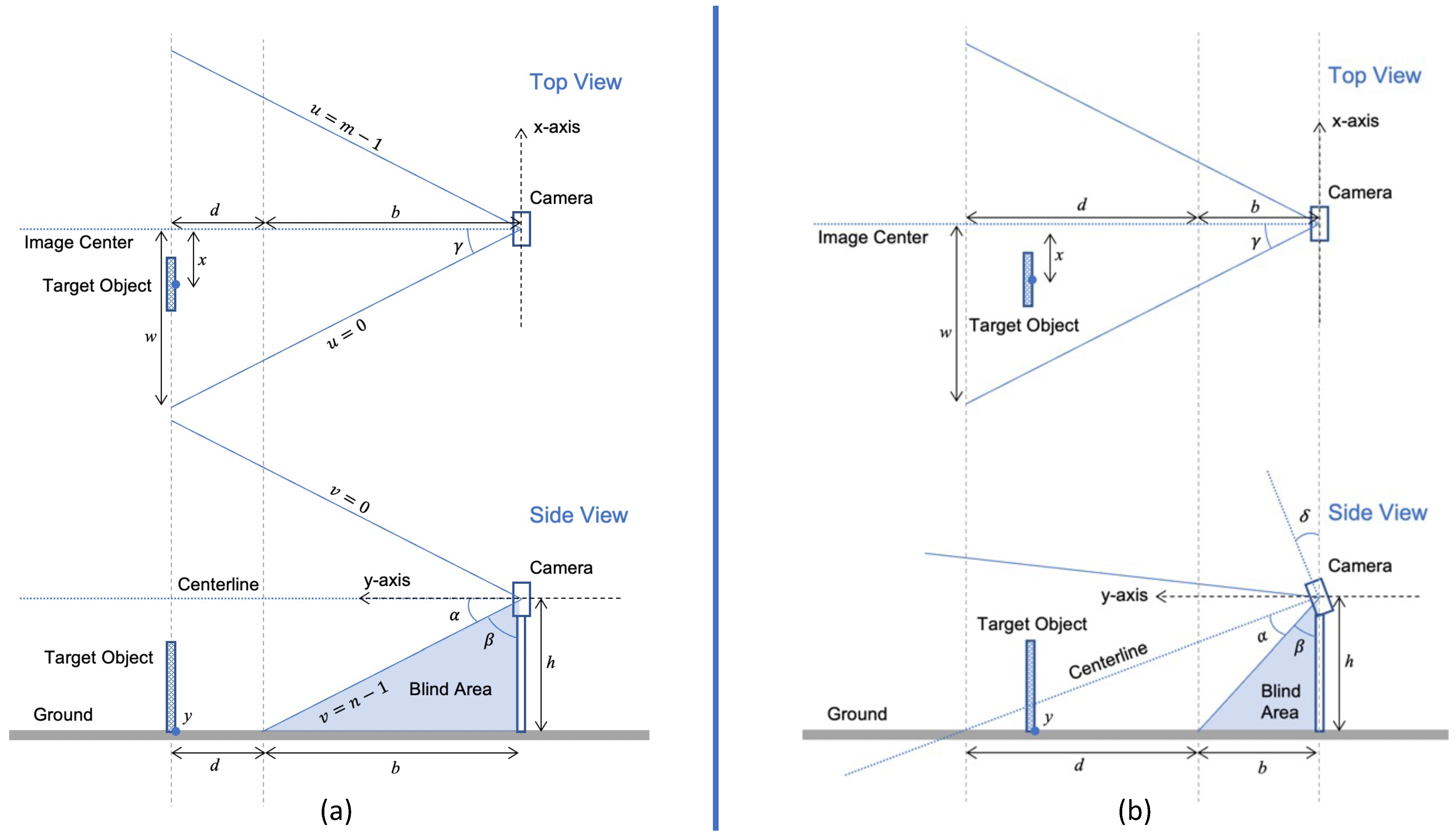
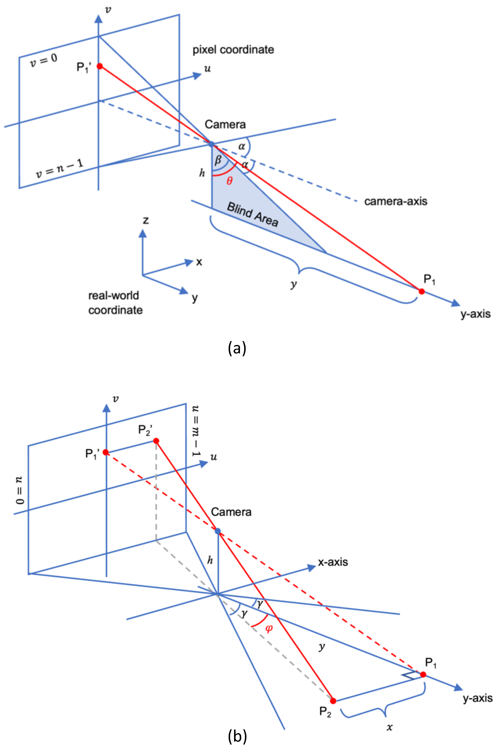
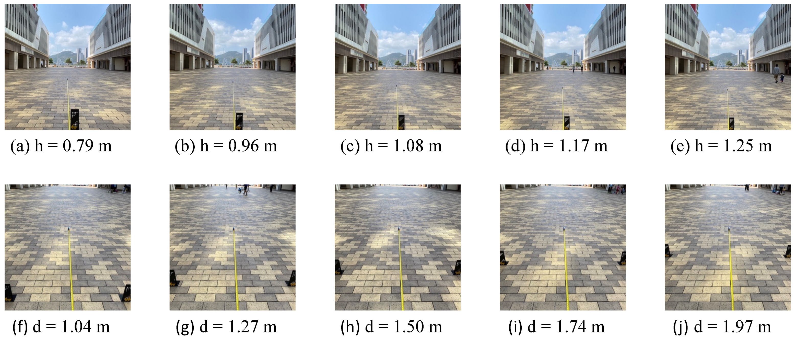
When a new camera is applied in the experiment, calibration is necessary for acquiring the camera’s FOV or focal length, which targets for the position-based estimation or size-based estimation. There are various methods to acquire the FOV. The calibration procedure in this experiment was as follows: (1) set up a camera on a tripod with the camera axis parallel to the ground; (2) place reference markings at particular locations according to the live view of the camera; (3) measure the location of reference markings in real-world coordinates; and (4) calculate the FOV of the camera from Equations (1)–(3). To acquire the vertical FOV of the camera, a tape measure was laid on the ground and extended from the bottom of the tripod along with the centerline of the camera. A distinguishable object was placed close to the edge in pixel coordinates (Figure 5a–e). Read from the tape measure to record the length of the blind area in real-world coordinates. Repeat the measurement at different heights to find the average.
Once the height of camera h and the length of bind area b were measured, β and α could be calculated by Equation (1). Hence, the average of vertical FOV of the camera used in the experiment is shown in Table 2.
For the horizontal FOV, similar steps were performed, but two objects were placed at the left and right edge in the pixel coordinate (Figure 5f–j). The camera was set up at a certain pitch angle, otherwise the width w would be too far away and close to the vanishing point if we set up the camera horizontally. The height of camera h was measured for calculating the actual distance d = ( d 2 + h 2 ) from the camera to the plane of w when the camera was hoisted at h. The horizontal FOV could be calculated by Equation (3). The average horizontal FOV of the camera in the experiment is shown in Table 3, where the height is fixed to 1.183 m.
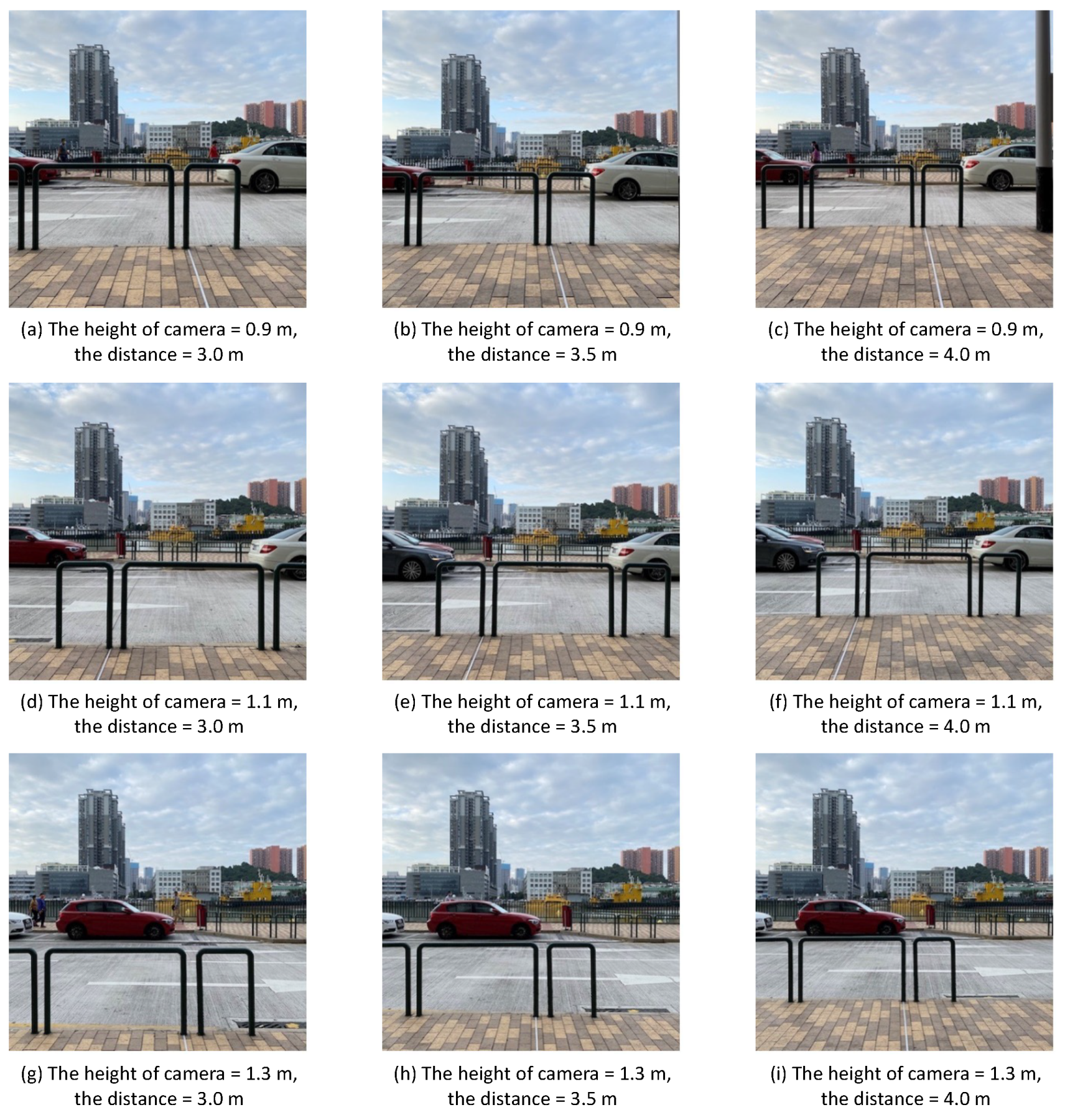
To acquire the focal length of the camera, take several pictures that contain the target objects at different distances (Figure 6). As long as the size of the objects and the distances are known, the focal length can be calculated by the following Equation (13).
f = h D H
where the height of the object in pixel h can be measured by photo editing software. Table 4 and Table 5 show a mean camera’s focal length of 424.52 by experiment.

4.2. Effective Distance

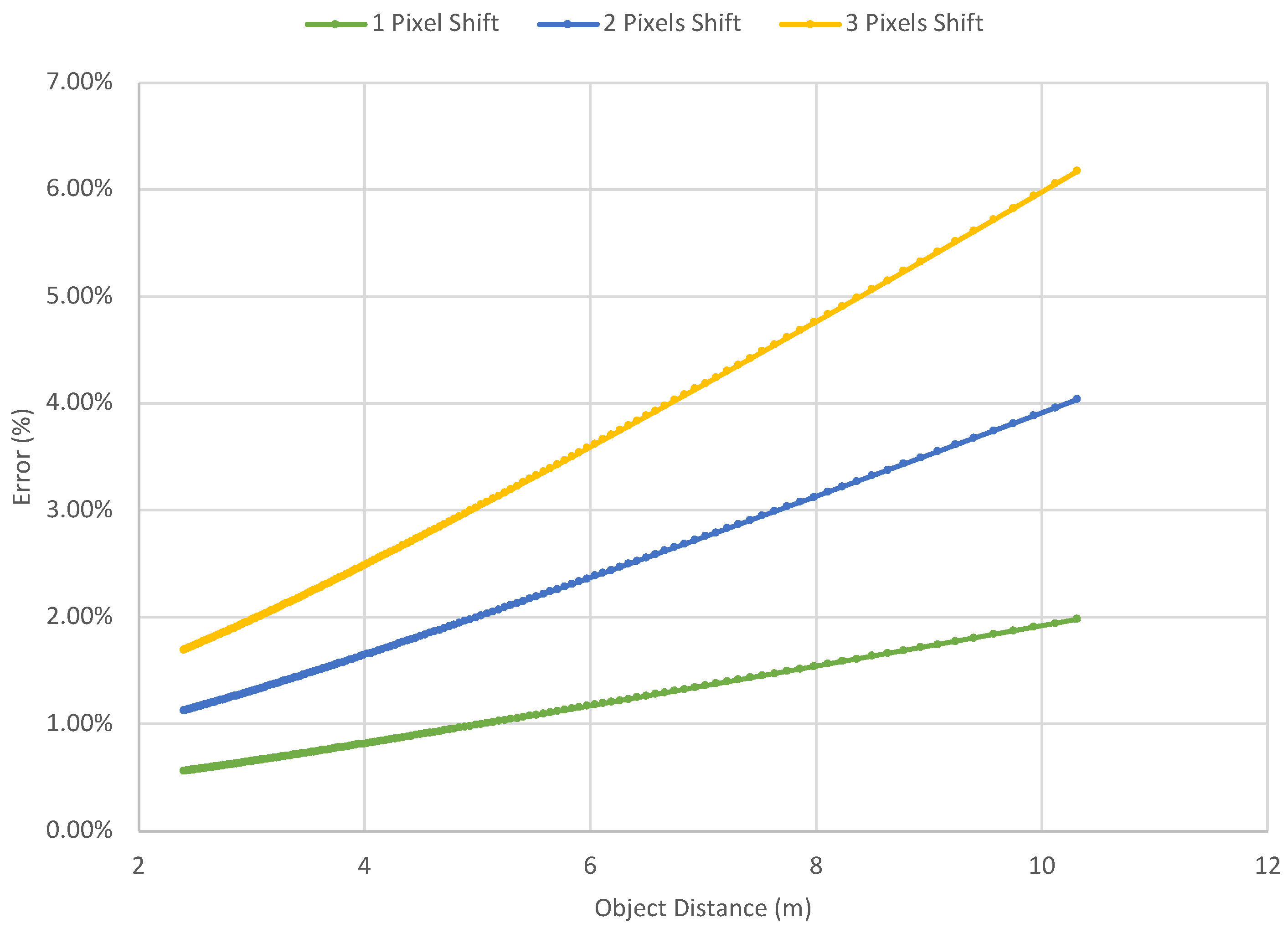
The error introduced by the pixel shift grows with the tangent function in the proposed model. For example, in our case a 416 × 416 image with a horizontal FOV of 63.46° and the camera height h = 1.2 m. Assuming the detection shifts 1 pixel at D = 2.4 m ( y = 0 in image coordinate),
y e r r = 1.2 × tan ( 63.46 + 2 × 26.54 × 1 416 ) 1.2 × tan ( 63.46 ) = 0.013 m
y e r r = y 156 y 155 = 0.196 m
In Equation (14), the error is 0.013 m, which is 0.56% of the distance. However, if 1-pixel shifting occurs at D = 10 m (y = 155 in image coordinate), the error becomes 0.196 m, which is 1.94% of the distance. Figure 7 illustrates the relationship between the object distance and the error introduced by the pixel shifting. For the object at 10 m, 2 to 3 pixels shifting made by the detection will introduce a 3.96% to 6.05% error. It is unignorable and it is necessary to define the effective distance for the proposed model.
According to Sørensen and Dederichs [39] and Bala et al. [
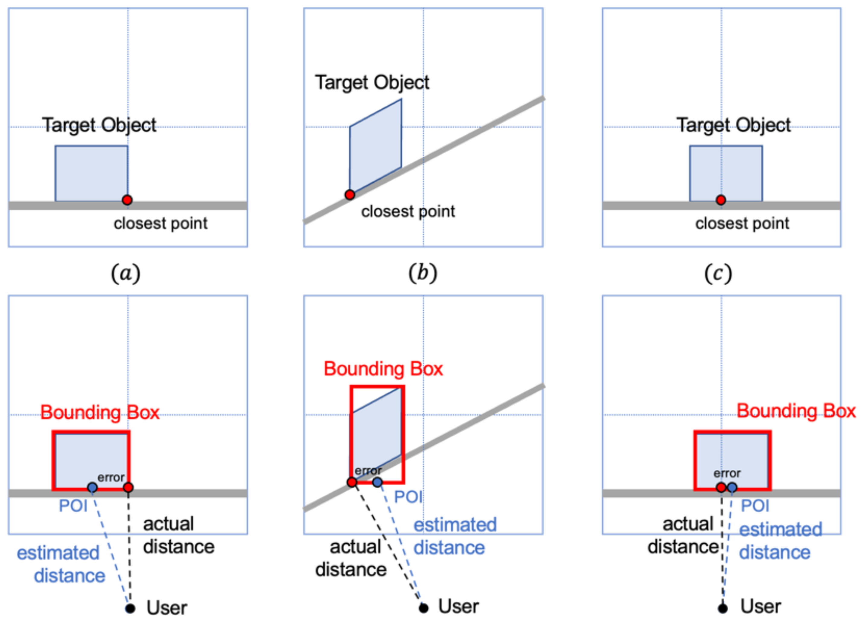
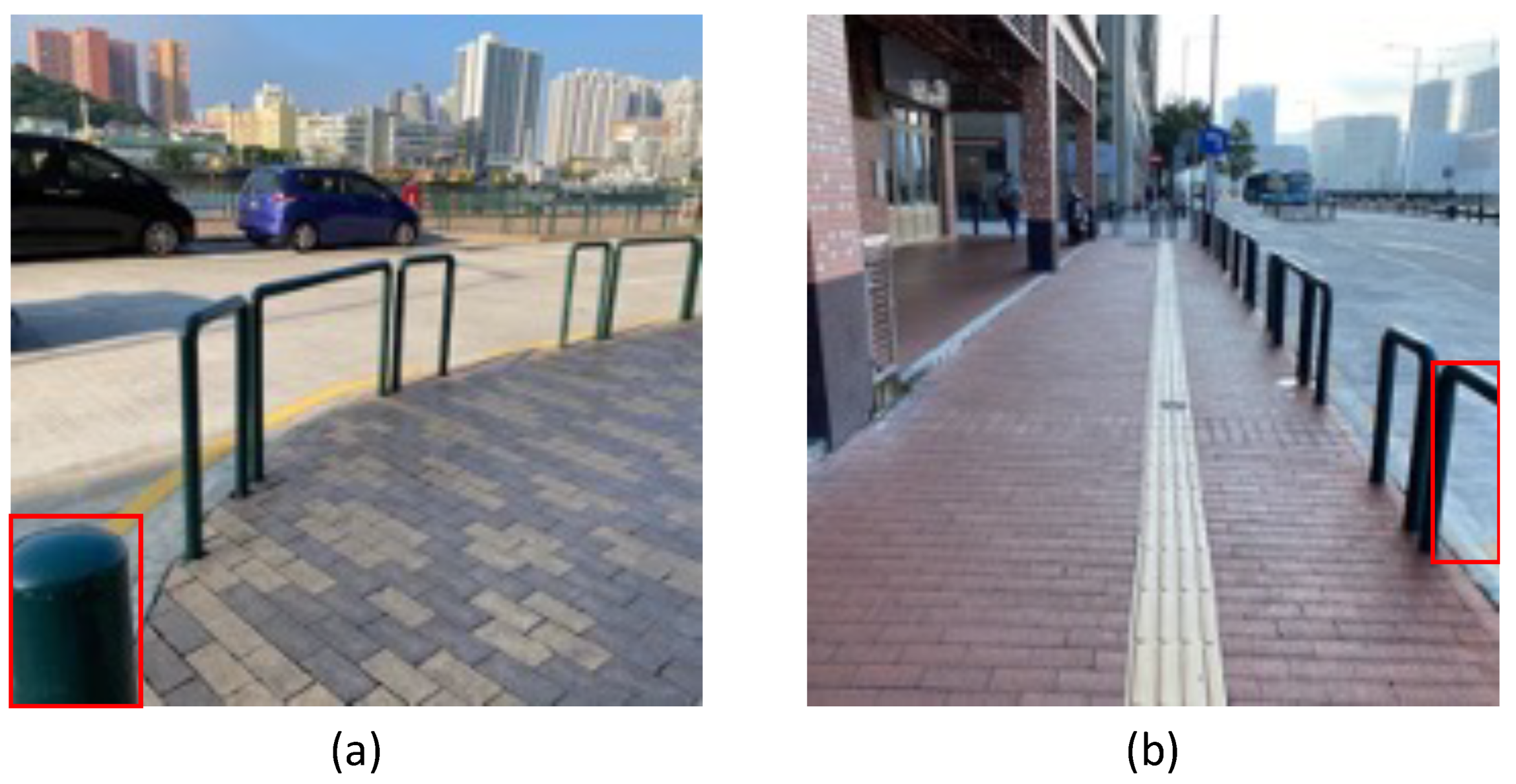
40], the mean walking speed of pedestrians is 1.69 m/s, 1.43 m/s, and 0.792 to 1.53 m/s for younger individuals, older individuals, and visually impaired people, respectively. Therefore, assuming there is an object located 10 m away, it takes 6.5 s (1.53 m/s) for the user to reach it. Assuming the system needs 0.5 s to manipulate, there are 6 s left for the users to respond and adjust their route. On the other hand, if a user is wearing a camera at 1.2 m height (average chest height of a human), the blind area is around 2.4 m. It means that the object closer than 2.4 m could not be or could only be partially detected. Since the position-based model is only effective for the object of which the bottom is completely captured, the partial detection will introduce error to the system (Figure 8). Hence, the effective distance of NFD is assumed to be 2.4 m to 10 m. For the estimation of the distance of objects shorter than the effective distance, it is suggested to use the previous frames of images for the determination.

4.3. Distance Estimation

In Table 6 and Table 7, all detected objects were classified into the correct class in the demonstration, thus the precision was 100%. The recall was up to 94.12% (YOLOv4-tiny) and 97.06% (YOLOv4) within the effective distance (<10 m). The mean absolute percentage error (MAPE) of distance estimation results within an effective distance was 6.18% (YOLOv4-tiny) and 6.24% (YOLOv4), respectively. The error of estimation out of effective distance (>10 m) was relatively large. The MAPE of all detections increased to 14.03% (YOLOv4-tiny) and 16.08% (YOLOv4). Some far objects (around 12 m) were estimated twice the distance to the ground truth due to pixel error. It proved that the proposed FOV model was not compatible with estimating far distance. The result was acceptable to a prototyping solution manipulating low-resolution images with the assumption of no distortion error. Based on the analysis, the errors were caused by two factors. (1) POI error, which could contribute to a maximum of 4% error; (2) bounding box error: since the average IoU of the model was 74.42% (YOLOv4-tiny) and 75.19% (YOLOv4). If a bounding box framed an object inner (or outer) its actual contour, the model would misjudge that the object was located farther (or closer) than its actual location, which is introduced by pixel shift.
To compare the performance between different distance estimation models, the trained deep learning model (80:20 split ratio, labeling method 2, and YOLOv4-tiny) was applied in the position-based (relying on the bottom of the object) and the size-based (relying on the height of the object) models, respectively. Table 8 summarizes the estimation results of the two models. The overall performance is shown in Table 9, in which the position-based model in short distances is better as the MAPE (within the effective distance) of the position-based model was 6.18%, but the size-based model was 6.59%. However, when taking the objects out of the effective distance into account, the size-based model gives a much better result. The MAPE of the size-based model was only 5.96% whereas the size-based model climbed to 14.03%. The size-based model shows the capability of estimating distance in dynamic range. Another advantage of the size-based model is that it is free from the assumption of the POI since it refers to the height of the detected objects. One of the limitations of the size-based model is that the detected object has to be completely detected. The misunderstanding of the sizes of occluded and partially out-of-view objects by the deep learning model will lead to a relatively large error. Therefore, a labeling method that ignores the incomplete target object is more suitable for the size-based distance estimation model.

4.4. Discussion and Future Work

The experiment shows that NFD provides a satisfying result in detecting selected near-front objects and estimating their distance from the user. It provides a relatively affordable solution for visually impaired people with the concept of ‘grab, wear, and go’. NFD utilized YOLOv4-tiny for object detection. It provides competitive performance in terms of accuracy among the other solutions for object detection. The training and inference speed outperform other solutions. However, the accuracy of distance estimation of NFD is not better than those with depth sensors, such as ToF cameras and LiDAR. However, inference output can directly locate detected objects in front at comparatively fewer resources (without going through the point cloud). On the other hand, using public objects, NFD can generally work in the entire city, whereas most of the existing solutions could only be utilized for indoor environments or particular areas. However, it can only recognize two types of outdoor public objects currently, implying that it can only work outdoors. Also, moving objects, such as humans and cars, are not detectable yet. To extend it, enhancing the dataset of the trained model for the improvement of the solution is needed in the future. The more high-quality data included in the dataset, the more accurate the prediction it can make using deep learning.
One of the improvements suggested to NFD is the dataset, which includes the image depth information from ToF or RGBD camera. Training images in the dataset can improve the accuracy of prediction, as bias from the lens model and camera posture can be ignored. Additionally, to enhance the robustness of NFD, other common public objects such as fire hydrants, street name signposts, traffic signs, streetlights, and especially humans and cars should be included in the object detection. Such an improved solution will be helpful to the vision-impaired people to fully understand the environment, locate themselves in the street, and avoid static and moving obstacles.

5. Conclusions

This study describes a novel distance estimate method that has undergone time-consuming, costly development, exact calibration, and thorough testing. This unique technique significantly lessens the computing load on edge application devices by utilizing mathematical models to produce reliable estimations. Our method represents a substantial development in the field since it incorporates modern object detection models. The testing results have shown that NFD estimate is accurate within the practical distance range. Based on the findings obtained from our experimental analysis, it is evident that the position-based model achieved a satisfactory mean absolute percentage error (MAPE) of 6.18%, whereas the size-based model yielded a slightly higher MAPE of 6.59%. Notably, both models exhibited commendable precision of 100% and a recall rate of 94.12% within a specified effective distance range of 2.4 to 10 m.
In ideal circumstances, where elements, including the camera’s alignment with the ground’s surface, minimum lens distortion, a well-defined effective distance, and exact POI are guaranteed, NFD emerges as a very effective navigation tool. It is also important to note that our suggested approach for distance estimate holds significant promise outside of its intended use cases. It has enormous promise for autopilot applications for electric cars and drone racing navigation, which advances computer vision and autonomous systems by offering insightful information on distance estimation in a dynamic 3D environment.
These promising findings imply that with further refinement, NFD can be embedded into a wearable device that provides real-time navigation support to those with visual impairments. This advancement allows visually impaired people to move and engage with their environment with greater independence and mobility. We are getting closer to achieving the full potential of this technology and changing the navigation help the market as we continue to refine it.

Author Contributions

Conceptualization, T.L.W., K.S.C. and K.L.W.; methodology, T.L.W., K.S.C. and K.L.W.; software, T.L.W., K.S.C. and K.L.W.; validation, D.A. and L.S.; formal analysis, T.L.W.; investigation, T.L.W., L.S., K.L.W. and K.S.C.; resource, R.T., S.-K.T. and G.P.; data curation, T.L.W.; writing—original draft preparation, T.L.W.; writing—review and editing, T.L.W., K.S.C., K.L.W., L.S., D.A., R.T., S.-K.T. and G.P.; visualization, T.L.W.; supervision, R.T., S.-K.T. and G.P.; project administration, R.T., S.-K.T. and G.P.; funding acquisition, R.T., S.-K.T. and G.P. All authors have read and agreed to the published version of the manuscript.

Funding

This research received no external funding.

Institutional Review Board Statement

Not applicable.

Informed Consent Statement

Not applicable.

Data Availability Statement

Not applicable.

Acknowledgments

This work is supported in part by the research grant (No.: RP/ESCA-04/2020) offered by Macao Polytechnic University.

Conflicts of Interest

The authors declare no conflict of interest.

References

  1. Li, C.; Zhu, B.; Zhang, J.; Guan, P.; Zhang, G.; Yu, H.; Yang, X.; Liu, L. Epidemiology, health policy and public health implications of visual impairment and age-related eye diseases in mainland China. Front. Public Health 2022, 10, 966006. [Google Scholar] [CrossRef]
  2. Bourne, R.R.; Adelson, J.; Flaxman, S.; Briant, P.; Bottone, M.; Vos, T.; Naidoo, K.; Braithwaite, T.; Cicinelli, M.; Jonas, J.; et al. Global Prevalence of Blindness and Distance and Near Vision Impairment in 2020: Progress towards the Vision 2020 targets and what the future holds. Investig. Ophthalmol. Visual Sci. 2020, 61, 2317. [Google Scholar]
  3. Messaoudi, M.D.; Menelas, B.A.J.; Mcheick, H. Review of Navigation Assistive Tools and Technologies for the Visually Impaired. Sensors 2022, 22, 7888. [Google Scholar] [CrossRef] [PubMed]
  4. Huang, C.Y.; Wu, C.K.; Liu, P.Y. Assistive technology in smart cities: A case of street crossing for the visually-impaired. Technol. Soc. 2022, 68, 101805. [Google Scholar] [CrossRef]
  5. Tse, R.; Mirri, S.; Tang, S.K.; Pau, G.; Salomoni, P. Modelling and Visualizing People Flow in Smart Buildings: A Case Study in a University Campus. In Proceedings of the Conference on Information Technology for Social Good, Association for Computing Machinery, GoodIT ’21, New York, NY, USA, 9–11 September 2021; pp. 309–312. [Google Scholar] [CrossRef]
  6. Rickly, J.M.; Halpern, N.; Hansen, M.; Welsman, J. Traveling with a guide dog: Confidence, constraints and affective qualities of the human-guide dog relationship. Tour. Manag. 2022, 93, 104617. [Google Scholar] [CrossRef]
  7. Zhu, J.; Hu, J.; Zhang, M.; Chen, Y.; Bi, S. A fog computing model for implementing motion guide to visually impaired. Simul. Model. Pract. Theory 2020, 101, 102015. [Google Scholar] [CrossRef]
  8. Zaidi, S.S.A.; Ansari, M.S.; Aslam, A.; Kanwal, N.; Asghar, M.; Lee, B. A survey of modern deep learning based object detection models. Digit. Signal Process. 2022, 126, 103514. [Google Scholar] [CrossRef]
  9. Xiao, Y.; Yin, S.; Cui, G.; Yao, L.; Fang, Z.; Zhang, W. A Near-Field Area Object Detection Method for Intelligent Vehicles Based on Multi-Sensor Information Fusion. World Electr. Veh. J. 2022, 13, 160. [Google Scholar] [CrossRef]
  10. Sukel, M.; Rudinac, S.; Worring, M. Urban object detection kit: A system for collection and analysis of street-level imagery. In Proceedings of the 2020 International Conference on Multimedia Retrieval, New York, NY, USA, 8–11 June 2020; pp. 509–516. [Google Scholar]
  11. Li, S.; Ozo, M.M.; Wagter, C.D.; de Croon, G.C. Autonomous drone race: A computationally efficient vision-based navigation and control strategy. Robot. Auton. Syst. 2020, 133, 103621. [Google Scholar] [CrossRef]
  12. Chou, K.S.; Wong, K.L.; Aguiari, D.; Tse, R.; Tang, S.K.; Pau, G. Recognition of Driving Behavior in Electric Vehicle’s Li-Ion Battery Aging. Appl. Sci. 2023, 13, 5608. [Google Scholar] [CrossRef]
  13. Tang, S.K.; Tse, R.; Lam, C.U. A new method of visualizing the road traffic: Differential timing method. In Proceedings of the Eleventh International Conference on Digital Image Processing (ICDIP 2019), Guangzhou, China, 10–13 May 2019; SPIE: Bellingham, WA, USA, 2019; Volume 11179, pp. 749–755. [Google Scholar]
  14. Chen, Y.; Tse, R.; Bosello, M.; Aguiari, D.; Tang, S.K.; Pau, G. Enabling deep reinforcement learning autonomous driving by 3D-LiDAR point clouds. In Proceedings of the Fourteenth International Conference on Digital Image Processing (ICDIP 2022), Wuhan, China, 20–23 May 2022; SPIE: Bellingham, WA, USA, 2022; Volume 12342, pp. 362–371. [Google Scholar]
  15. Wong, T.L.; Chou, K.S.; Wong, K.L.; Tang, S.K. Dataset of Public Objects in Uncontrolled Environment for Navigation Aiding. Data 2023, 8, 42. [Google Scholar] [CrossRef]
  16. Vernimmen, R.; Hooijer, A.; Pronk, M. New ICESat-2 satellite LiDAR data allow first global lowland DTM suitable for accurate coastal flood risk assessment. Remote Sens. 2020, 12, 2827. [Google Scholar] [CrossRef]
  17. Szeliski, R. Computer Vision: Algorithms and Applications; Springer Nature: Berlin/Heidelberg, Germany, 2022. [Google Scholar]
  18. Scharstein, D.; Szeliski, R. A taxonomy and evaluation of dense two-frame stereo correspondence algorithms. Int. J. Comput. Vis. 2002, 47, 7–42. [Google Scholar] [CrossRef]
  19. Stein, G.P.; Mano, O.; Shashua, A. Vision-based ACC with a single camera: Bounds on range and range rate accuracy. In Proceedings of the IEEE IV2003 Intelligent Vehicles Symposium, Proceedings (Cat. No. 03TH8683), Columbus, OH, USA, 9–11 June 2003; IEEE: Piscataway, NJ, USA, 2003; pp. 120–125. [Google Scholar]
  20. Park, K.Y.; Hwang, S.Y. Robust range estimation with a monocular camera for vision-based forward collision warning system. Sci. World J. 2014, 2014, 923632. [Google Scholar] [CrossRef] [PubMed]
  21. Tram, V.T.B.; Yoo, M. Vehicle-to-vehicle distance estimation using a low-resolution camera based on visible light communications. IEEE Access 2018, 6, 4521–4527. [Google Scholar] [CrossRef]
  22. Chen, Y.C.; Su, T.F.; Lai, S.H. Integrated vehicle and lane detection with distance estimation. In Proceedings of the Computer Vision-ACCV 2014 Workshops, Singapore, 1–2 November 2014; Revised Selected Papers, Part III 12. Springer: Berlin/Heidelberg, Germany, 2015; pp. 473–485. [Google Scholar]
  23. Eigen, D.; Puhrsch, C.; Fergus, R. Depth map prediction from a single image using a multi-scale deep network. Adv. Neural Inf. Process. Syst. 2014, 27. [Google Scholar]
  24. Garg, R.; Bg, V.K.; Carneiro, G.; Reid, I. Unsupervised cnn for single view depth estimation: Geometry to the rescue. In Proceedings of the Computer Vision–ECCV 2016: 14th European Conference, Amsterdam, The Netherlands, 11–14 October 2016; Proceedings, Part VIII 14. Springer: Berlin/Heidelberg, Germany, 2016; pp. 740–756. [Google Scholar]
  25. Zhou, T.; Brown, M.; Snavely, N.; Lowe, D.G. Unsupervised learning of depth and ego-motion from video. In Proceedings of the IEEE Conference on Computer Vision and Pattern Recognition, Honolulu, HI, USA, 21–26 July 2017; pp. 1851–1858. [Google Scholar]
  26. Ye, C.; Qian, X. 3-D object recognition of a robotic navigation aid for the visually impaired. IEEE Trans. Neural Syst. Rehabil. Eng. 2017, 26, 441–450. [Google Scholar] [CrossRef] [PubMed]
  27. Kayukawa, S.; Takagi, H.; Guerreiro, J.; Morishima, S.; Asakawa, C. Smartphone-based assistance for blind people to stand in lines. In Proceedings of the Extended Abstracts of the 2020 CHI Conference on Human Factors in Computing Systems, Honolulu, HI, USA, 25–30 April 2020; pp. 1–8. [Google Scholar]
  28. Ying, J.C.; Li, C.Y.; Wu, G.W.; Li, J.X.; Chen, W.J.; Yang, D.L. A deep learning approach to sensory navigation device for blind guidance. In Proceedings of the 2018 IEEE 20th International Conference on High Performance Computing and Communications, the IEEE 16th International Conference on Smart City, the IEEE 4th International Conference on Data Science and Systems (HPCC/SmartCity/DSS), Exeter, UK, 28–30 June 2018; pp. 1195–1200. [Google Scholar]
  29. Shelton, A.; Ogunfunmi, T. Developing a deep learning-enabled guide for the visually impaired. In Proceedings of the 2020 IEEE Global Humanitarian Technology Conference (GHTC), Seattle, WA, USA, 29 October–1 November 2020; IEEE: Piscataway, NJ, USA, 2020; pp. 1–8. [Google Scholar]
  30. Ryan, J.; Okazaki, D.; Dallow, M.; Dezfouli, B. NavSense: A Navigation Tool for Visually Impaired. In Proceedings of the 2019 IEEE Global Humanitarian Technology Conference (GHTC), Seattle, WA, USA, 17–20 October 2019; IEEE: Piscataway, NJ, USA, 2019; pp. 1–8. [Google Scholar]
  31. Sohl-Dickstein, J.; Teng, S.; Gaub, B.M.; Rodgers, C.C.; Li, C.; DeWeese, M.R.; Harper, N.S. A device for human ultrasonic echolocation. IEEE Trans. Biomed. Eng. 2015, 62, 1526–1534. [Google Scholar] [CrossRef]
  32. LabelImg. LabelImg: A Graphical Image Annotation Tool to Label Object Bounding Boxes in Images. Available online: https://morioh.com/a/adff27290f5e/labelimg-is-a-graphical-image-annotation-tool-and-label-object-bounding-boxes-in-images (accessed on 6 September 2023).
  33. Bisong, E. Google Colaboratory. In Building Machine Learning And Deep Learning Models on Google Cloud Platform: A Comprehensive Guide for Beginners; Apress: Berkeley, CA, USA, 2019; pp. 59–64. [Google Scholar] [CrossRef]
  34. FAQ, D. Programming Comments—Darknet FAQ. Available online: https://www.ccoderun.ca/programming/darknet_faq/ (accessed on 6 September 2023).
  35. Redmon, J.; Divvala, S.; Girshick, R.; Farhadi, A. You Only Look Once: Unified, Real-Time Object Detection. In Proceedings of the 2016 IEEE Conference on Computer Vision and Pattern Recognition (CVPR), Las Vegas, NV, USA, 27–30 June 2016; IEEE: Piscataway, NJ, USA, 2016. [Google Scholar]
  36. Taylor, T.; Geva, S.; Boles, W. Monocular vision as a range sensor. In Proceedings of the International Conference on Computational Intelligence for Modelling, Control & Automation (CIMCA 2004), University of Canberra, Bruce, ACT, Australia, 12–14 July 2004; pp. 566–575. [Google Scholar]
  37. Shin, H.; Oh, S.; Hong, S.; Kang, M.; Kang, D.; Ji, Y.g.; Choi, B.H.; Kang, K.W.; Jeong, H.; Park, Y.; et al. Early-stage lung cancer diagnosis by deep learning-based spectroscopic analysis of circulating exosomes. ACS Nano 2020, 14, 5435–5444. [Google Scholar] [CrossRef]
  38. Qi, S.; Li, J.; Sun, Z.; Zhang, J.; Sun, Y. Distance estimation of monocular based on vehicle pose information. J. Phys. Conf. Ser. 2019, 1168, 032040. [Google Scholar] [CrossRef]
  39. Sørensen, J.G.; Dederichs, A.S. Evacuation characteristics of visually impaired people—A qualitative and quantitative study. Fire Mater. 2015, 39, 385–395. [Google Scholar] [CrossRef]
  40. Bala, M.M.; Vasundhara, D.; Haritha, A.; Moorthy, C.V. Design, development and performance analysis of cognitive assisting aid with multi sensor fused navigation for visually impaired people. J. Big Data 2023, 10, 21. [Google Scholar] [CrossRef]
Figure 1. The overall architecture of NFD. The NFD modeling procedure calibrates the device camera to obtain the ground truth of the object distance and estimate the FOV on the bounding boxes image after YOLOv4 detection.
Applsci 13 11038 g001
Figure 2. Camera positioning. (a) Scenario of holding the camera horizontally. (b) Scenario of camera setup at an arbitrary pitch angle.
Applsci 13 11038 g002
Figure 3. Distance estimation using triangulation relationship. (a) A point ( P 1 ) on the y-axis in real coordinate and its projection in pixel coordinate ( P 1 ). (b) A point ( P 2 ) shifting along the x-axis and its projection in pixel coordinate ( P 2 ).
Applsci 13 11038 g003
Figure 4. Image view of POI and bounding box. (a) an object is perpendicular to the camera axis and located in the left half of the image; (b) an object is oblique to the camera axis and located in the left half of the image; (c) an object is perpendicular to the camera axis and locates across the centerline of the image. It is difficult to determine the closest point of the object from the information of the bounding box.
Applsci 13 11038 g004
Figure 5. Experiments for acquiring the camera’s vertical and horizontal FOV.
Applsci 13 11038 g005
Figure 6. Experiments for acquiring the camera’s focal length.
Applsci 13 11038 g006
Figure 7. Relationship of object distance and error by pixel shift (h = 1.2 m).
Applsci 13 11038 g007
Figure 8. Example of partially out-of-view objects. (a) Only the upper part of the pillar was detected. The system could not estimate its distance; (b) only half of the fence was detected. The POI indicated by the bounding box is far from the closest point of the object. Both cases introduce errors into the system.
Applsci 13 11038 g008
Table 1. Comparison between NFD and existing solutions.
Existing SolutionTechnique/ModelHardwareTarget ObjectAdvantagesDisadvantages
Ye and Qian [26]3D point cloud3D ToF camera & tabletStructural Object (e.g., doorway, hallway, stairway, ground, and wall)Highly accurate and possible to combine with SLAM/wayfinding solutionsHigh computing resources required and indoor only
Kayukawa et al. [27]YOLOv3-tinySmartphone (built-in RGB camera and infrared depth camera)HumanHigh mobility and off-the-shelf device requiredVery specific application and short distance
Ying et al. [28]YOLOv3Stereo webcam & NVIDIA Jetson TX2Indoor furniture (e.g., chair and table)Low cost but small dataset requiredLow mobility and accuracy in distance estimation
Shelton and Ogunfunmi [29]AlexNetWebcam & laptopIndoor objects and outdoor buildingsText-to-speech function involved, available in both indoor and outdoorOnly workable in the authors’ campus and low mobility
Ryan et al. [30]MobileNet-SSDv2Micro-controllers, Raspberry PiCam & webcam, ultrasonic & infrared ToF SensorGeneral objects (VOC and COCO dataset)High mobility, available in low power, and low costAdditional sensors for distance estimation required. Implemented with the existing navigation tool
Sohl-Dickstein et al. [31]Ultrasonic echolocationSpeaker & ultrasonic microphonesAny object in short distanceWork without visible light, provide 3D spatial informationShort distance and could not recognize objects
Table 2. Readings of vertical FOV experiments.
 h (m)b (m) β α Vertical FOV
(a)0.7941.5663.03°26.97°53.95°
(b)0.9591.8862.97°27.03°54.05°
(c)1.0792.1563.35°26.65°53.30°
(d)1.1672.3963.97°26.03°52.05°
(e)1.2542.5763.99°26.01°52.02°
  Average:63.46°26.54°53.07°
Table 3. Readings of horizontal FOV experiments.
 d (m)w (m) γ Horizontal FOV
(f)1.0401.37523.58°47.16°
(g)1.2701.59624.69°49.38°
(h)1.5001.78225.00°50.01°
(i)1.7351.98225.26°50.53°
(j)1.9652.18725.49°50.98°
  Average:24.81°49.61°
Table 4. Readings of focal length experiment on long fence height.
 Camera Height (m)Distance (m)Height (Pixel)Focal Length (Pixel/m)
(a)0.93.0120418.60
(b)0.93.5103419.19
(c)0.94.089413.95
(d)1.13.0123429.07
(e)1.13.5105427.33
(f)1.14.092427.91
(g)1.33.0122425.58
(h)1.33.5103419.19
(i)1.34.092427.91
Table 5. Readings of focal length experiment on short fence height.
 Camera Height (m)Distance (m)Height (Pixel)Focal Length (Pixel/m)
(a)0.93.0121422.09
(b)0.93.5104423.26
(c)0.94.090418.6
(d)1.13.0125436.05
(e)1.13.5103419.19
(f)1.14.092427.91
(g)1.33.0122425.58
(h)1.33.5105427.33
(i)1.34.093432.56
Table 6. Estimated distance in the demonstration.
TestObjGround Truth (m)YOLOv4-TinyYOLO-v4
ClassEstimated Distance (m)ErrorClassEstimated Distance (m)Error
114.5304.50−0.66%04.50−0.66%
25.1315.201.36%15.150.39%
37.2107.402.64%07.280.97%
47.8017.931.67%18.012.69%
59.0009.030.33%08.95−0.56%
610.05N--210.221.69%
710.49N--211.065.43%
213.0303.112.64%03.102.31%
23.1513.356.35%13.407.94%
314.1404.02−2.90%04.00−3.38%
24.7114.66−1.06%14.55−3.40%
36.7106.03−10.13%06.02−10.28%
414.3004.576.28%04.453.49%
24.3814.564.11%14.512.97%
34.4804.674.24%04.807.14%
513.6303.722.48%03.743.03%
24.1914.364.06%14.394.77%
35.5506.089.55%06.038.65%
47.3908.2611.77%08.3412.86%
58.0319.4818.06%19.1814.32%
69.38N--N--
614.5104.673.55%04.745.10%
24.3324.657.39%24.688.08%
34.7225.2411.02%25.2611.44%
411.89020.5973.17%019.4363.41%
511.82018.0953.05%018.1253.30%
611.76N--218.5057.31%
711.88N--220.1569.61%
812.15023.5994.16%022.5385.43%
912.28125.72109.45127.86126.87%
713.8803.86−0.52%03.84−1.03%
24.4514.593.15%14.501.12%
35.8006.288.28%06.267.93%
47.5808.4611.61%08.339.89%
58.1519.3314.48%19.2313.25%
69.64N--011.2817.01%
711.56N--N--
812.21N--114.5018.76%
813.7313.50−6.17%13.781.34%
23.8203.71−2.88%03.80−0.52%
34.7125.067.43%25.067.43%
45.3425.818.80%25.778.05%
513.33N--216.9727.31%
612.85N--216.3627.32%
712.67N--215.7824.55%
812.72N--215.6623.11%
913.86017.1823.95%016.5219.19%
1014.53N--117.9923.81%
913.6823.29−10.60%23.28−10.87%
23.7523.32−11.47%23.26−13.07%
311.11N--210.67−3.96%
411.13N--210.37−6.83%
511.33010.61−6.35%010.81−4.59%
611.28011.310.27%010.87−3.63%
712.10011.72−3.14%012.05−0.41%
“N” denotes the absence of detected objects. The blue highlights indicate objects beyond the effective range, while the red highlights represent false negatives within the effective distance.
Table 7. Estimated distance by the different models.
TestObjGround Truth (m)ClassPosition-BasedSize-Based
Estimated Distance (m)ErrorEstimated Distance (m)Error
114.5304.50−0.66%4.06−10.38%
25.1315.201.36%4.51−12.09%
37.2107.402.64%7.02−2.64%
47.8017.931.67%7.30−6.41%
59.0009.030.33%8.69−3.44%
610.05N----
710.49N----
213.0303.112.64%2.94−2.97%
23.1513.356.35%3.09−1.90%
314.1404.02−2.90%3.69−10.87%
24.7114.66−1.06%4.2−10.83%
36.7106.03−10.13%5.79−13.71%
414.3004.576.28%4.42.33%
24.3814.564.11%4.564.11%
34.4804.674.24%4.35−2.90%
513.6303.722.48%3.26−10.19%
24.1914.364.06%3.72−11.22%
35.5506.089.55%5.53−0.36%
47.3908.2611.77%7.450.81%
58.0319.4818.06%8.698.22%
69.38N----
614.5104.673.55%3.92−13.08%
24.3324.657.39%4.350.46%
34.7225.2411.02%4.4−6.78%
411.89020.5973.17%12.172.35%
511.82018.0953.05%11.06−6.43%
611.76N----
711.88N----
812.15023.5994.16%11.77−3.13%
912.28125.72109.4511.77−4.15%
713.8803.86−0.52%3.38−12.89%
24.4514.593.15%3.88−12.81%
35.8006.288.28%5.7−1.72%
47.5808.4611.61%7.60.26%
58.1519.3314.48%7.94−2.58%
69.64N----
711.56N----
812.21N----
813.7313.50−6.17%3.07−17.69%
23.8203.71−2.88%3.26−14.66%
34.7125.067.43%4.81.91%
45.3425.818.80%5.07-5.06%
513.33N----
612.85N----
712.67N----
812.72N----
913.86017.1823.95%14.041.30%
1014.53N----
913.6823.29−10.60%3.762.17%
23.7523.32−11.47%3.883.47%
311.11N----
411.13N----
511.33010.61−6.35%11.06−2.38%
611.28011.310.27%11.06−1.95%
712.10011.72−3.14%11.41−5.70%
“N” denotes the absence of detected objects. The blue highlights indicate objects beyond the effective range, while the red highlights represent false negatives within the effective distance.
Table 8. Performance on object detection models.
MethodsMAPE (within Effective Distance)MAPEPrecisionRecall (within Effective Distance)Recall
YOLOv4-tiny6.18%14.03%100%94.12%72.72%
YOLO-v46.24%16.08%100%97.06%96.36%
Table 9. Performance on distance estimation models.
ModelsMAPE (within Effective Distance)MAPE
Position-based6.18%14.03%
Size-based6.59%5.96%
Disclaimer/Publisher’s Note: The statements, opinions and data contained in all publications are solely those of the individual author(s) and contributor(s) and not of MDPI and/or the editor(s). MDPI and/or the editor(s) disclaim responsibility for any injury to people or property resulting from any ideas, methods, instructions or products referred to in the content.

