Improved YOLOv4-Tiny Target Detection Method Based on Adaptive Self-Order Piecewise Enhancement and Multiscale Feature Optimization

Abstract

To improve the accuracy of material identification under low contrast conditions, this paper proposes an improved YOLOv4-tiny target detection method based on an adaptive self-order piecewise enhancement and multiscale feature optimization. The model first constructs an adaptive self-rank piecewise enhancement algorithm to enhance low-contrast images and then considers the fast detection ability of the YOLOv4-tiny network. To make the detection network have a higher accuracy, this paper adds an SE channel attention mechanism and an SPP module to this lightweight backbone network to increase the receptive field of the model and enrich the expression ability of the feature map. The network can pay more attention to salient information, suppress edge information, and effectively improve the training accuracy of the model. At the same time, to better fuse the features of different scales, the FPN multiscale feature fusion structure is redesigned to strengthen the fusion of semantic information at all levels of the network, enhance the ability of network feature extraction, and improve the overall detection accuracy of the model. The experimental results show that compared with the mainstream network framework, the improved YOLOv4-tiny network in this paper effectively improves the running speed and target detection accuracy of the model, and its mAP index reaches 98.85%, achieving better detection results.

1. Introduction

With the development of science and technology and the maturity of artificial intelligence technology, All industries are moving in the direction of intelligence. As one of the important pillar industries in China, construction machinery has played a vital role in the development of construction infrastructure in China [1]. Construction machinery covers infrastructure, mining, and other fields. The working environment is relatively bad, often accompanied by a high temperature, dust, vibration, etc. The complex working environment poses a serious threat to the safety of workers; part of the work of construction machinery is highly repetitive, and the working area is relatively fixed. Therefore, reducing the safety risk caused by construction machinery operation, saving labor cost, and developing unmanned and intelligent construction machinery have an important practical significance. According to the work requirements of construction machinery, this paper carried out research on technology for the intelligent identification of engineering materials in complex environments, realized the intelligent identification of construction machinery and material categories by loaders, and made independent decisions according to the surrounding environment to improve work efficiency and ensure the work safety of staff.

In recent years, with the development of computer hardware, target detection algorithms based on deep convolution neural network [2,3] have developed rapidly and have been widely used in various industries. These kinds of algorithms can learn target features from a large number of images and have the characteristics of a high detection accuracy and a good robustness. It is an important research direction in the field of computer vision. In the process of material identification, the material features are not prominent and obvious, which directly affects the final identification accuracy. Therefore, to fully mine the details of the image to ensure the accuracy of recognition, it is necessary to enhance the contrast of low-contrast image to improve the quality of the image. After increasing its clarity, the image is combined with a convolution neural network to improve the accuracy of recognition. To date, many experts and scholars have proposed many contrast enhancement algorithms based on different theoretical foundations. Most of these algorithms can effectively enhance the contrast of the image, thereby improving the visual effect of the image [4]. For example, the wavelet-based homomorphic filter proposed by Zhang et al. [5], the S-function image contrast enhancement algorithm based on human eye brightness perception proposed by Wang et al. [6], and the low-illumination image contrast enhancement algorithm based on the retinex theory proposed by Zhang et al. [7] have achieved good results in processing image contrast. This provides a good theoretical basis for the adaptive color scale enhancement algorithm proposed in this paper. This model mainly performs a color scale enhancement pretreatment on the collected data such as foggy days and dark environments, highlighting the target features in the scene, and providing a good basis for neural network training. The target detection algorithm based on convolutional neural network is mainly divided into a two-stage target detection algorithm and a one-stage target monitoring algorithm. A two-stage target detection algorithm first forms a target candidate frame and then detects the target through a convolution neural network. The detection accuracy is high, but the real-time performance is poor. Representative methods include R-CNN [8], Fast R-CNN [9], etc. A single-stage detection algorithm detects the target directly by a convolution neural network without generating the target candidate frame in advance. The detection accuracy of that method is lower than that of a two-stage algorithm, but the detection speed is faster. Representative methods include YOLO [10], SSD [11], etc.

At present, the YOLO algorithm is applied in practical projects by more and more people because of its excellent detection speed. Wu et al. applied the improved YOLOv4-tiny to the target recognition of a transmission line [12], redesigned the network for the problems of large-scale changes of targets around transmission lines, many small targets, and easy-to-miss reports, effectively improving the detection accuracy of the model. Fu Bowen et al. applied the improved YOLOv4-tiny to the rapid detection of face key points [13]. Compared with other methods, the proposed model had a higher recognition efficiency and lower configuration requirements based on ensuring the recognition accuracy. Zhao et al. applied the improved YOLOv4 algorithm to vehicle detection [14]. Aiming at the problem of the low detection accuracy in complex environments, the void convolution and focal loss function were introduced into the network to effectively solve the problem of a large difference between positive and negative samples in the detection process, and the accuracy was improved by 7.31% compared with that of the original method. Leng et al. applied an improved YOLOv4 in their research on traffic sign recognition [15], which effectively alleviated the problem of the low recognition accuracy caused by small targets and a complex background of traffic sign targets, and the average accuracy rate was nine percentage points higher than that of the original YOLOv4. Sun et al. applied an improved YOLOv4-tiny to pedestrian target detection in a school [16] and replaced the deep separable convolution with an ordinary convolution, reducing the complexity of the model. Compared with the original method, that method had the advantages of a high accuracy, fast speed, less parameters, and it could be applied to embedded devices. Liu et al. applied an improved YOLOv4-tiny to solder joint detection [17]. Compared with the original method, the average accuracy of the improved algorithm reached 99.3%, and the detection speed reached 91 f/s. Liu et al. proposed a lightweight contraband detection method based on YOLOv4 for X-ray security inspection, which utilized MobilenetV3 to replace the backbone network of YOLOv4, while optimizing the neck and head of YOLOv4 using a depth-separable convolution, significantly reducing the computational and parametric quantities [18]. Yu et al. proposed YOLOv4-FPM for the real-time detection of bridge cracks, using a pruning algorithm to simplify the network and speed up the detection, with an mAP of 97.6% and a reduced model size and number of parameters [19]. Zhang et al. combined GhostNet with coordinate attention to improve YOLOv4 and improved the mAP by 3.45% and the detection speed by 5.7 FPS on a dense apple detection task [20].

In order to be able to meet the work needs of unmanned loaders, it is important to study a material recognition algorithm that can be used in complex working conditions. At present, the YOLOv4-tiny algorithm, as a first-stage target detection algorithm, has greater advantages in detection speed and detection accuracy. However, the detection capability of YOLOv4-tiny is affected by low-contrast environments such as dark scenes and rainy and foggy weather, and the lower the contrast, the worse the detection effect is, which can cause the detection to fail. In order to enhance the problem of a poor detection of construction machinery and materials in low-contrast environments, we propose to enhance the collected low-contrast images by using an adaptive self-order segmentation enhancement algorithm, which makes the processed images clearer and the target contours more obvious. Then, we improve the YOLOv4-tiny network structure, the backbone feature extraction network by using an SE attention mechanism and an SPP module, and the FPN feature fusion structure to further improve the detection of construction machinery and materials.

The main contributions of this paper are as follows:

(1)

In the processing of image contrast, the adaptive piecewise self-order enhancement model proposed in this paper has a remarkable effect. The image color scale information is completely corrected, the target contrast is clear, the peak signal-to-noise ratio (PSNR) of the image before and after correction reaches more than 145, and the structural similarity of the image before and after correction can reach more than 95%.

(2)

By adding a spatial pyramid pooling module to the algorithmic feature extraction network, the feature information under different sense field sizes can be fused, and the fused feature maps contain different levels of semantic information, which is helpful to improve the abstract expression of features.

(3)

An attention mechanism is incorporated in the network, which can adaptively adjust the weights of each channel, enabling the network to focus more on important information and suppress irrelevant information in the channel dimension, increasing detection accuracy while ensuring an almost constant training time and detection speed.

(4)

The FPN feature pyramid fusion structure is improved, and a fusion mode is added to the original basis to realize a bidirectional connection, enhance the effective fusion of shallow and deep information, improve the utilization of multiscale features, and enrich the information in the feature map.

(5)

Finally, compared with the original algorithm, the improved YOLOv4-tiny target detection algorithm shows some improvement in the average precision of detection. The mAP reaches 98.85%.

2. Adaptive Piecewise Self-Order Enhancement Algorithm

To improve the detection rate of the algorithm, we carried out an adaptive self-order color scale enhancement on the collected low-contrast images to improve the images’ clarity and highlight the contour features of the target. The relevant enhancement principles are as follows.

2.1. Principle of Traditional Piecewise Enhancement Algorithm

The traditional piecewise enhancement algorithm divides the gray level of the image into three parts through the maximum and minimum gray limits of the image gray level. When the pixel value is less than the minimum gray value, the pixel gray value is assigned to 0, indicating that the pixel has no color component in the gray class, so as to weaken the gray level. If the pixel gray level is greater than the maximum gray value, the pixel is assigned a value of 255 to achieve the purpose of enhancing the gray level. When the pixel is larger than the minimum gray level but smaller than the maximum gray level, the gray level of the pixel is normalized to complete the gray level enhancement of the image. The specific model is as follows:

$$map\left(i+1\right)=\left\{\begin{array}{c}0\begin{array}{cc},& i<\mathrm{m}\mathrm{i}\mathrm{n}\left(R\right)\end{array}\hfill \\ uint8\left(\frac{\left(i-\mathrm{m}\mathrm{i}\mathrm{n}\left(R\right)\right)}{\left(\mathrm{m}\mathrm{a}\mathrm{x}\left(R\right)-\mathrm{m}\mathrm{i}\mathrm{n}\left(R\right)\right)}\right)\times 255\begin{array}{cc},& \mathrm{m}\mathrm{i}\mathrm{n}\left(R\right)\le i\le \mathrm{m}\mathrm{a}\mathrm{x}\left(R\right)\end{array}\hfill \\ 255\begin{array}{cc},& i>\mathrm{m}\mathrm{a}\mathrm{x}\left(R\right)\end{array}\hfill \end{array}\right.$$

(1)

where $map$ represents the defined pixel size, the i of $map(i+1)$ represents a pixel in image I, $\mathrm{m}\mathrm{a}\mathrm{x}\left(R\right)$ and $\mathrm{m}\mathrm{i}\mathrm{n}\left(R\right)$, respectively, represent the maximum and minimum gray values of the image.

2.2. Adaptive Piecewise Self-Order Enhancement Algorithm

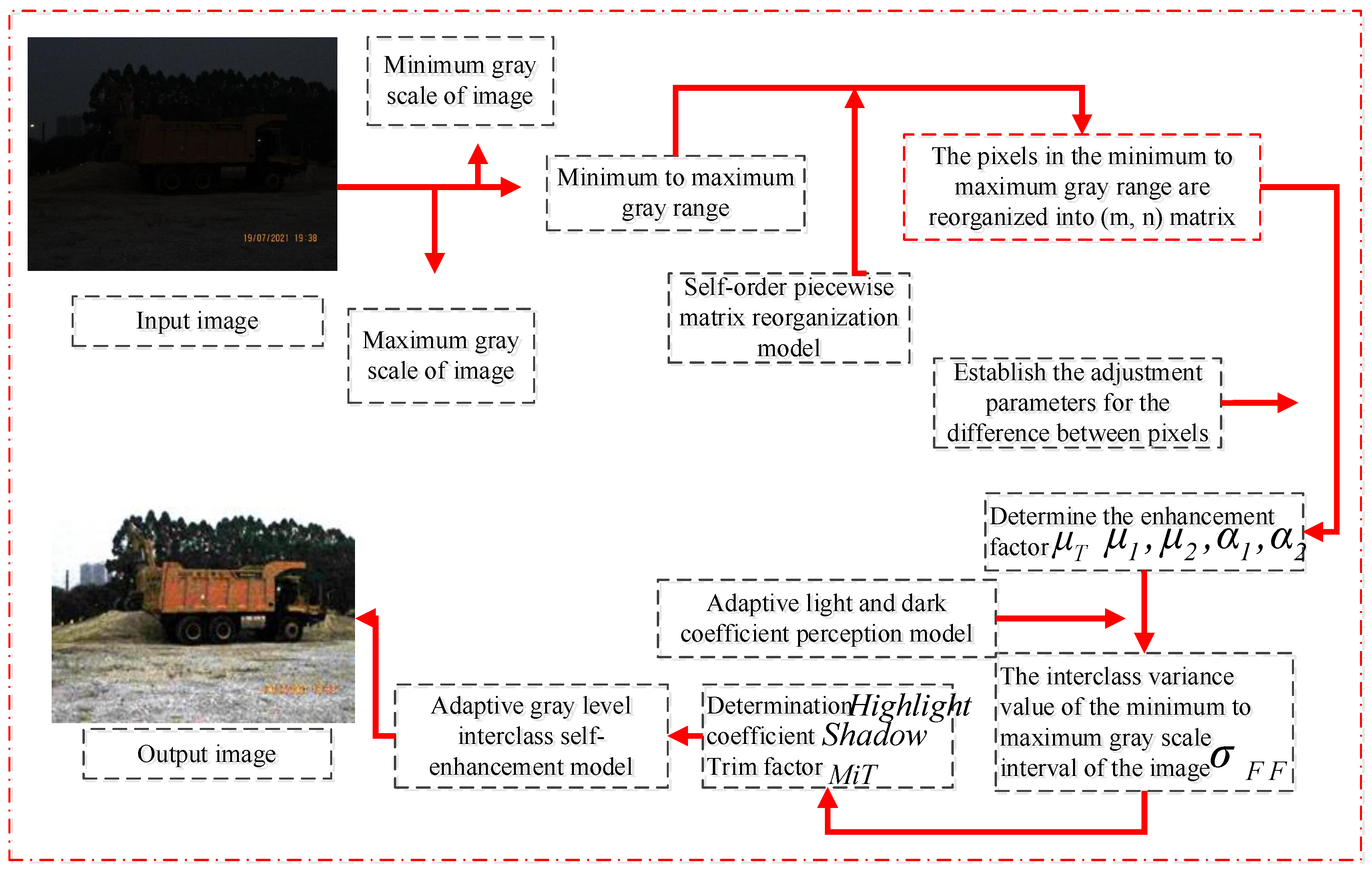
In the image gray level enhancement algorithm of the traditional self-ranking algorithm, the image pixel enhancement is mainly based on the maximum interclass difference of the image gray level. In the study of Formula (1) above, it is found that the simple algorithm for the gray level enhancement that adjusts the relevant fixed parameters through prior knowledge uniformly uses a simple normalization to enhance the pixels between the minimum gray level and the maximum gray level. The utilization rate of the interclass gray level information of the image is not high, resulting in a poor image enhancement effect, and the distinction between dark and bright gray levels in the image is polarized. Therefore, in view of the shortcomings of the image enhancement produced by the simple processing in the above formula, this paper constructed a self-order matrix reorganization analysis model to perform an interclass enhancement on the gray levels of the intermediate stage. The image can be enhanced according to different gray intensities, and the gray difference information between each gray level can be fully used to improve the quality of the image after the enhancement. The specific model is as follows:

$$map\left(i+1\right)=\left\{\begin{array}{c}255\begin{array}{cc},& i>\mathrm{m}\mathrm{a}\mathrm{x}\left(R\right)\end{array}\hfill \\ data\begin{array}{cc},& \mathrm{m}\mathrm{i}\mathrm{n}\left(R\right)\le i\le \mathrm{m}\mathrm{a}\mathrm{x}\left(R\right)\end{array}\hfill \\ 0\begin{array}{cc},& i<\mathrm{m}\mathrm{i}\mathrm{n}\left(R\right)\end{array}\hfill \end{array}\right.$$

(2)

In the formula, $data\left[\right]$ refers to the pixel stored between the minimum pixel and the maximum pixel. Other definitions are as shown in Formula (1). In this operation, all pixels smaller than the minimum and larger than the maximum are defined as 0 and 255 gray levels. For pixels larger than the minimum and smaller than the maximum, the defined reorganization model is as follows:

$$Data=reshape(data,m,n)$$

(3)

In the formula, $Data$ represents the pixel matrix after the matrix reorganization of the image gray levels, $reshape$ represents the element reorganization function, $data$ represents the result in Formula (2), $(m,n)$ represents the pixel matrix with a size of the element reorganization of $m\times n$. In order to effectively use the gray level between the minimum value and the maximum value of a pixel to reflect the interclass difference between the gray levels of each pixel and finally realize the gray level enhancement of the pixel, firstly, the histogram analysis of the reconstructed gray pixel is as follows:

$$DataR=imshist\left(Data\right)/(m\times n)$$

(4)

In the formula, $DataR$ represents the histogram after image normalization, and the other parameters are defined as above. The interclass coefficient of the gray level ${\mu }_T$ in the histogram can be determined by defining the gray level $colorlevel=256$ of the pixel according to the image as follows:

$${\mu }_T={\mu }_T+colorlevel\left(j\right)\times DataR\left(j\right)$$

(5)

In the formula, ${\mu }_T$ refers to the gray level coefficient in the range from the minimum gray level to the maximum gray level. The initial value is defined as 0, which means the defined gray level is from 1 to 256. In order to achieve the adaptive gray level enhancement, the difference between pixel classes must be adjusted by determining various gray level enhancement parameters ${\mu }_1,{\mu }_2,{\alpha }_1,{\alpha }_2$ adaptively according to the defined gray level $colorlevel$. The model for determining each parameter is as follows:

$$\left\{\begin{array}{c}{\alpha }_1={\alpha }_1+DataR\left(j_1\right)\hfill \\ {\alpha }_2=1-{\alpha }_1\hfill \end{array}\right.$$

(6)

$$\left\{\begin{array}{c}{\mu }_1={\mu }_1+\left(j_2-1\right)\times DataR\left(j_2\right)\begin{array}{cc}& \left(j_2<Th\right)\end{array}\hfill \\ {\mu }_2={\mu }_2+\left(j_2-1\right)\times DataR\left(j_2\right)\begin{array}{cc}& \left(j_2>Th\right)\end{array}\hfill \\ {\mu }_1={\mu }_1/{\alpha }_1\hfill \\ {\mu }_2={\mu }_2/{\alpha }_2\hfill \end{array}\right.$$

(7)

In the formula, ${\mu }_1,{\mu }_2,{\alpha }_1,$ and ${\alpha }_2$ represent the difference between adaptive gray levels according to the image information, $Th$ represents the adaptive gray level value, $DataR$ represents the result of the operation in Formula (4), $j_1$ and $j_2$ represent the cyclic operation parameters of the gray level $colorlevel$, where $j_1=1\sim (th-1)$, $(Th=colorlevel-1),j_2=1\sim colorlevel$.

Finally, the interclass variance of the output image of Formulas (5)–(7) is used as the judgment condition for the enhancement, and its mathematical model is as follows:

$${\sigma }_{FF}={\alpha }_1\times {\left({\mu }_1-{\mu }_T\right)}^2+{\alpha }_2\times {\left({\mu }_2-{\mu }_T\right)}^2$$

(8)

${\mu }_T$ represents the gray scale coefficient calculated in Formula (5) from the minimum gray scale to the maximum gray scale. Other definitions are as follows.

In order to make effective use of the information of the interclass gray level of the image for the enhancement, this paper proposes an adaptive light–dark perception model to build the model based on the parameters of the adjustment of the interclass difference, the variance of the interclass difference, and the original light–dark difference of the image. The specific model is as follows:

$$Highlight=\left\{\begin{array}{c}{\sigma }_{FF}\times 1.5\begin{array}{cc},& 100\le {\sigma }_{FF}<150\end{array}\hfill \\ {\sigma }_{FF}\times 4.5\begin{array}{cc},& {\sigma }_{FF}\ge 150\end{array}\hfill \\ {\sigma }_{FF}\times 4\begin{array}{cc},& {\sigma }_{FF}<100\end{array}\hfill \end{array}\right.$$

(9)

In the formula, ${\sigma }_{FF}$ is the maximum gray value of each gray category calculated in Formula (8) in the original image. Because this paper focused on the gray enhancement of dark night scenes with a low contrast and foggy weather scenes with a high brightness, it makes sense to choose different $Highlight$ parameters for the operation of grayscale enhancement according to the brightness of different scenes. At the same time, this paper used the brightness difference of each gray level in the original image to reflect the shadow characteristics between each gray level and obtained the brightness difference of the overall image through the difference between the highest brightness level of the image and the overall shadow coefficient of the image. The overall brightness difference of the image and the brightness difference between the image’s gray classes were combined and normalized to increase the information utilization rate of the image. The perception model of shadow parameters in this paper was as follows:

$$Shadow=ceil\left(\frac{\mathrm{m}\mathrm{a}\mathrm{x}\left(\mathrm{a}\mathrm{l}\mathrm{l}\left({\sigma }_{FF}\right)\right)}{\mathrm{m}\mathrm{i}\mathrm{n}\left(\mathrm{a}\mathrm{l}\mathrm{l}\left({\sigma }_{FF}\right)\right)}\right)$$

(10)

In the formula, $ceil$ it is the upward rounding function, and $\mathrm{a}\mathrm{l}\mathrm{l}\left({\sigma }_{FF}\right)$ represents the interclass variance value of all gray levels of the image. In addition, in order to effectively improve the information utilization rate and image enhancement effect, this paper also set the corresponding fine-tuning parameters to adapt the fine-tuning image enhancement effect based on different brightness levels and different scenes. The specific model was as follows:

$$MiT=\left\{\begin{array}{c}Highlight/1000\begin{array}{cc},& Highlight\ge 200\end{array}\hfill \\ 1\begin{array}{cc},& Highlight<200\end{array}\hfill \end{array}\right.$$

(11)

In the formula, $Highlight$ represents the overall brightness of the image. When it is a foggy scene, the gray levels of the pixels are similar, so the fine adjustment coefficient $MiT$ should be far less than 1. In a dark scene, there is a large difference between the gray level of the target pixel and the overall background, so it is necessary to improve the fine adjustment coefficient $MiT$ to enhance the color scale recovery effect. This paper defined its value as 1.

In combination with the parameters established by the above corresponding models, the enhancement model proposed in this paper is as follows:

$$D(i,j)=\left\{\begin{array}{c}Highlight-\left({\sigma }_{FF}\right)/255\begin{array}{cc},& \mathrm{m}\mathrm{i}\mathrm{n}\left[data(:)\right]\le Data(i,j)\le \mathrm{m}\mathrm{a}\mathrm{x}\left[data(:)\right]\end{array}\hfill \\ Highlight-Shadow\hfill \end{array}\right.$$

(12)

$$D_r(i,j)=\left\{\begin{array}{c}Data(i,j)-\left({\sigma }_{FF}\right)/255\begin{array}{cc},& D(i,j)=Highlight-\left({\sigma }_{FF}\right)/255\end{array}\hfill \\ Data(i,j)-Shadow\begin{array}{cc},& D(i,j)=Highlight-Shadow\end{array}\hfill \\ 0\begin{array}{cc},& D_r\le 0\end{array}\hfill \end{array}\right.$$

(13)

$$Result(i,j)={\left(\frac{D_r(i,j)}{D(i,j)}\right)}^{\left(\frac{1}{MiT}\right)\times 255}$$

(14)

In the formula, $Data(i,j)$ means that the grayscale value of the image between the maximum and minimum grayscale, $\mathrm{m}\mathrm{i}\mathrm{n}\left[data\right(:\left)\right]$, $\mathrm{m}\mathrm{a}\mathrm{x}\left[data\right(:\left)\right]$ means the minimum and maximum gray levels of the image, respectively. $Highlight$ represents the brightness of the image, $Shadow$ represents the shadow parameter of the image, $D(i,j)$ represents the brightness difference of a certain gray level in the whole image, ${\sigma }_{FF}$ denotes the operation result of Formula (8), $D_r$ represents the average gray level difference of the gray level, $(i,j)$ denotes the coordinates of the image element, and $Result(i,j)$ is the final enhancement result of the gray level. The overall process and pseudocode of the algorithm are as follows:

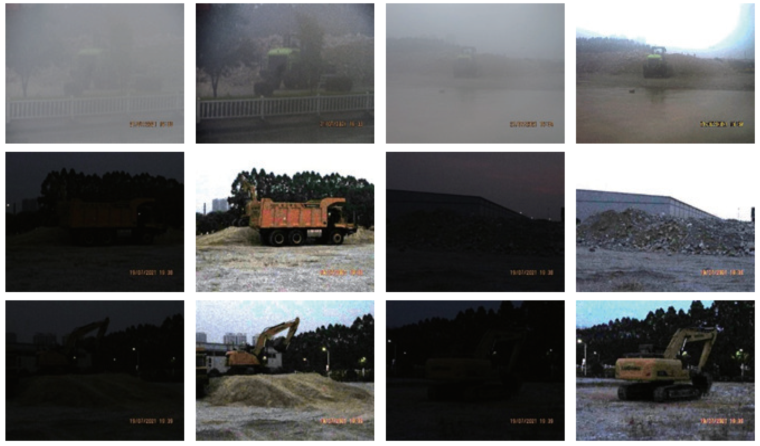
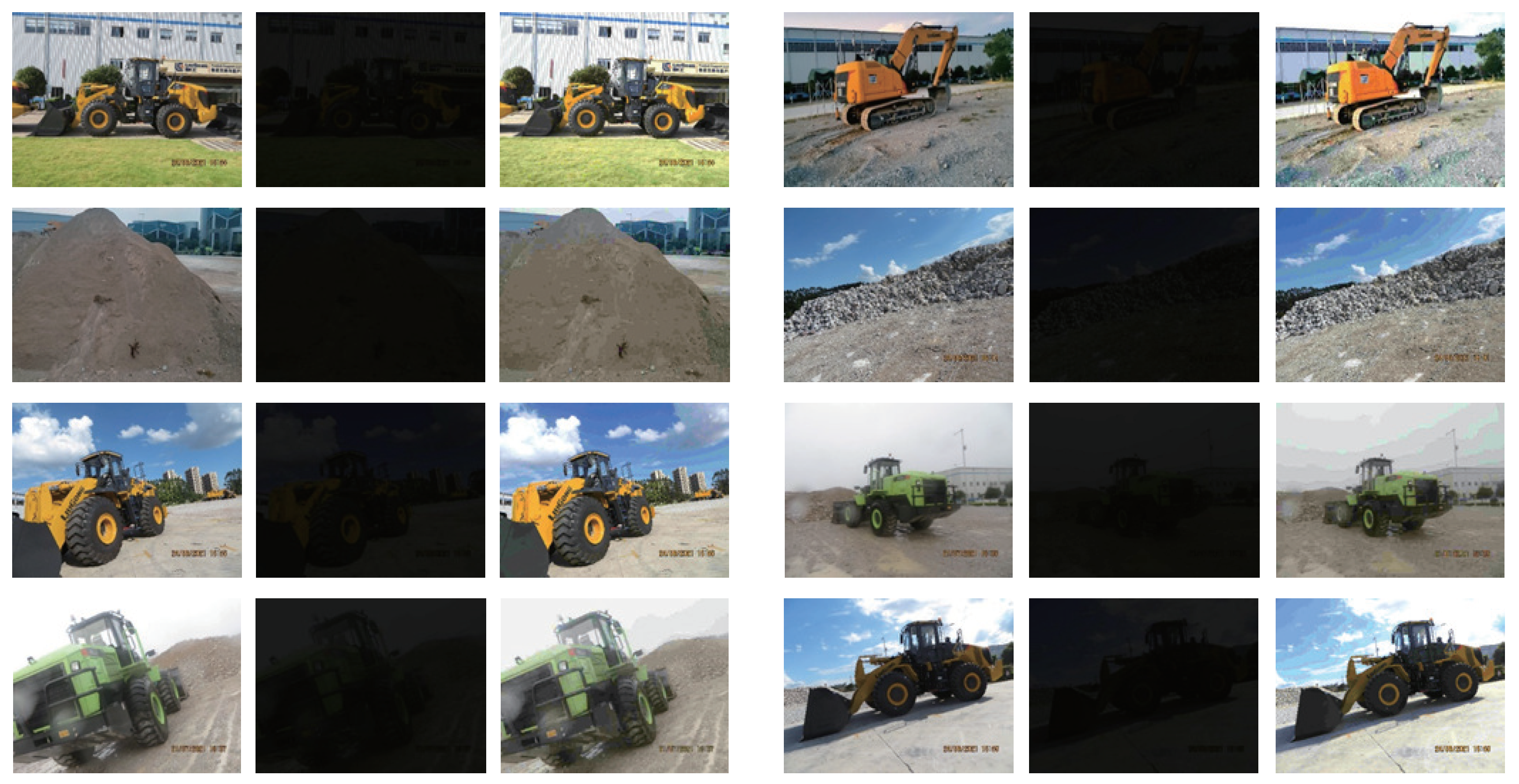
As shown in Figure 1 below, the image enhancement effect of the algorithm proposed in this paper is obtained after preliminary verification. It can be seen from the figure that the image enhancement effect of the algorithm proposed in this paper is obvious. The pseudocode of the overall algorithm is shown in

Table 1. Proposed algorithm pseudocode.

Step 1. Input image I;

Step 2. Use Formula (1) to obtain the histogram of the pixel gray distribution in input image I and calculate its maximum and minimum values $\min R$;

Step 3. On the basis of step 2, combine Formula (2) to count and normalize the pixels in the range from the minimum pixel to the maximum pixel values of each gray level category in the image;

Step 4. Reorganize the pixel whose gray level is in the minimum to maximum range into a new operational matrix $Data$ using Formula (3);

Step 5. Calculate the result of step 4 and Formulas (4)–(8), and output the adaptive self-order parameters of gray scale ${\sigma }_F$

Step 6. Combine Formulas (9)–(11) to determine the adaptive brightness parameters $Highlight$, scene shadows $Shadow$, and fine-tune parameters $MiT$ for different scenes;

Step 7. Combining the operation results and Formulas (12)–(14) in steps 5 and 6, complete the preliminary image preprocessing to achieve the purpose of darkening the foggy image and for a preliminary enhancement of the dark night image;

Step 8. Defining the image brightness parameter $Highlight=50$, the scene shadow $Shadow$ is defined as the result of Formula (9) divided by 65,535, and the fine-tuning parameter is defined as $Mi0.8$;

Step 9. Combine the results in steps 7 and 8 with those in steps 3, 4, and 5 to output the corresponding adaptive parameters, and then combine them with Formulas (12)–(14) to output the final enhancement results.

:

3. Improved YOLOv4-Tiny Detection Model

3.1. Basic Principle of YOLOv4-Tiny

The YOLO algorithm is a popular one-stage detection algorithm. The algorithm treats the target detection problem as a regression problem. The convolution neural network structure can directly predict the location and category of the target, it runs fast, and it can achieve real-time detection. YOLOv4 [21], as one of the most advanced algorithms in the current YOLO series, is an improvement of YOLOv3 [22]. It has strong real-time performance and a high accuracy and has been widely used in practical projects. YOLOv4-tiny is a lightweight network version of YOLOv4, which simplifies the network structure and parameter quantity. Its detection accuracy is lower than that of YOLOv4 but it has a higher detection speed. It also has obvious advantages in detection speed and accuracy compared with other versions of the YOLOv4 lightweight network. Its network structure is shown in Figure 2. The research goal of this paper was to achieve the classification and detection tasks of 9 types of targets. The detection speed and accuracy of the algorithm were high. Because the target scale of construction machinery and materials is large, and the number of categories is small, it does not need too deep a convolution neural network, so we chose to improve the YOLOv4-tiny algorithm.

YOLOv4-tiny uses CSP Darknet53-tiny as the backbone network, with a (416 × 416)-size image used as input. The backbone network is mainly composed of the CBL module and CSPBlock residual module. The CBL module is composed of a common convolution layer (Conv), batch standardization (BN), and leaky ReLu activation function. The CSPBlock module divides the input features into two parts. When stacking the residual blocks, a large residual edge is introduced. Finally, the two feature maps are spliced and the combined feature maps are downsampled using maximum pooling. This structure can effectively reduce the number of calculations. After downsampling 16 times and 32 times, the high-level and low-level feature information are fused using the idea of a feature pyramid [23] to improve the network-free feature extraction ability, and the final output size is 13 × 13 and 26 × 26 for the target detection.

The YOLOv4-tiny algorithm first extracts the features of the input image through the feature extraction network and then divides it into S × S grid cells. If the center point of a target falls in the grid cell, the grid is responsible for predicting the target. Each grid cell needs to predict three boundary boxes. Each boundary box contains information on four positions, x, y, w, and h, as well as the confidence and probability of a category. Multiple grid cells may predict the same target, Therefore the results are filtered using non-maximum suppression to get the coordinates and categories of the detected targets.

YOLOv4-tiny’s loss function refers to the difference between the predicted value of the model and the real value. The smaller the value of the loss function, the higher the prediction accuracy and the better the robustness of the model. YOLOv4-tiny’s loss function includes three parts, namely, the position loss, the confidence loss, and the category loss. The loss function is shown in Equation (15).

$$\mathrm{Loss}=L_{\mathrm{CIOU}}+L_{\mathrm{conf}}+L_{cls}$$

(15)

$$L_{CIOU}={\lambda }_{coord}\sum _{i=0}^{K\times K}\sum _{j=0}^M{I}_{ij}^{obj}\left(2-w_i\times h_i\right)\left(1-CIOU\right)$$

(16)

$$CIOU=IOU-\frac{{\rho }^2(b,b^{gt})}{c^2}-\beta v$$

(17)

$$\beta =\frac{v}{1-IOU+v}$$

(18)

$$v=\frac{4}{{\pi }^2}{\left(\arctan \frac{w^{gt}}{h^{gt}}-\arctan \frac{w}{h}\right)}^{{}^2}$$

(19)

$$\begin{gathered} \begin{array}{c}{L}_{conf}={\displaystyle \sum _{i=0}^{K\times K}}{\displaystyle \sum _{j=0}^M}{I}_{ij}^{obj}\left[{\stackrel{⌢}{C}}_i\mathrm{l}\mathrm{o}\mathrm{g}\left(C_i\right)+(1-{\stackrel{⌢}{C}}_i)\mathrm{l}\mathrm{o}\mathrm{g}(1-C_i)\right]\hfill \end{array}- \\ {\lambda }_{noobj}\sum _{i=0}^{K\times K}\sum _{j=0}^M{I}_{ij}^{noobj}\left[{\stackrel{⌢}{C}}_i\mathrm{l}\mathrm{o}\mathrm{g}\left(C_i\right)+(1-{\stackrel{⌢}{C}}_i)\mathrm{l}\mathrm{o}\mathrm{g}(1-C_i)\right] \end{gathered}$$

(20)

$$L_{cls}=-\sum _{i=0}^{K\times K}\sum _{j=0}^M{I}_{ij}^{obj}\sum _{c\in classes}\left[{\stackrel{⌢}{p}}_i\left(c\right)\mathrm{l}\mathrm{o}\mathrm{g}\left(p_i\left(c\right)\right)+\left(1-{\stackrel{⌢}{p}}_i\left(c\right)\right.\right)\mathrm{l}\mathrm{o}\mathrm{g}(1-p_i\left(c\right))]$$

(21)

In the above formula, $L_{CIOU}$ is the location loss, $L_{conf}$ is the confidence loss, and $L_{cls}$ is the category loss. In $L_{CIOU}$, ${\lambda }_{coord}$ is the weight coefficient of positive samples, ${\displaystyle \sum _{i=0}^{K\times K}}{\displaystyle \sum _{j=0}^M}$ means traversing all the prediction boxes, $I_{ij}^{obj}$ determines whether the sample is positive or not, where a positive sample is 1 and a negative sample is 0. ${\rho }^2(b,b^{gt})$ denotes the Euclidean distance between the prediction frame and the center point of the real frame. c denotes the diagonal distance of the smallest closed region containing both the predicted and real boxes, $\beta$ is a parameter measuring the consistency of the aspect ratio, and v is the trade-off parameter. $\left(2-w_i\times h_i\right)$ is the penalty term, $w_i$ and $h_i$ are the width and height of the center point of the prediction box, $w^{gt}$ and $h^{gt}$ are the width and height of the real frame, and w and h are the width and height of the prediction box. $L_{conf}$ and $L_{cls}$ are calculated using the cross-entropy loss, $I_{ij}^{noobj}$ is used to determine whether the judgment is a negative sample, where the negative sample is 1 and the positive sample is 0. ${\lambda }_{noobj}$ is the negative sample weighting factor.

3.2. Improved YOLOv4-Tiny Algorithm

Because the detection algorithm in this paper was aimed at the detection and classification of construction machinery and materials, the target scale changed little, the category was small and had obvious characteristic information. The deep convolution neural network model had too many parameters and a long training time, which was not suitable for this project. Therefore, we chose to improve YOLOv4-tiny, a lightweight model, in order to achieve a higher detection accuracy under the condition of ensuring a faster detection speed.

The improved YOLOv4-tiny in this paper added a channel attention SE module [24] and a spatial pyramid pooling module to the original network and improved the FPN feature fusion part of the network. The details are as follows: (1) At the neck of the network structure, this paper added an SPP module [25]. The SPP module is composed of four parallel branches, each with a convolution core size of 5 × 5, 9 × 9, 13 × 13, and a jump connection. Finally, the feature maps of the four branches are spliced and transferred to the next layer. The SPP module draws on the idea of the spatial pyramid, which enables the convolutional neural network to input images of arbitrary size, use different sliding window sizes and step sizes for different output scales, and finally output a fixed-length vector, realizing the fusion of local features and global features. Moreover, the fused feature map contains different levels of semantic information, which is conducive to improving the abstract expression of features and enhancing the sensitivity of features to high-level semantic concepts. (2) To make the detection network have higher accuracy, we inserted a channel attention mechanism SE module between the backbone feature extraction network and the feature fusion network. The SE module first performs a squeeze operation through a global average pooling to compress the input feature map of each channel into a scalar. This process can be regarded as feature extraction for each channel to obtain the importance of the channel. Then, the squeezed feature vector is input into two fully connected layers through the excitation operation. One fully connected layer is used to learn the weights between channels, and the other fully connected layer is used to learn the activation function. Then, the outputs of the two fully connected layers are multiplied to obtain a channel attention vector. Finally, the channel attention vector is applied to the input feature map to enhance useful features and weaken useless features. Its main advantages are that it can adaptively adjust the weight of each channel so that useful features get a higher weight and useless features get a lower weight, thereby improving the accuracy and robustness of the model. It can effectively improve the accuracy of the target detection with a small increase in the number of parameters. (3) In YOLOv4-tiny, the main role of the FPN structure is to solve the multiscale target detection problem in target detection by extracting multiscale features from different levels of feature maps, so that targets of different sizes can be detected. To be able to better fuse the features of different scales, we redesigned the FPN multiscale feature fusion structure. In the original structure, the multiscale features were fused only once. In this algorithm, we used a top-down and bottom-up bidirectional fusion based on the original fusion, using upsampling and downsampling to unify the features to the same size and adding jump connections between same-scale feature maps to realize the fusion of higher-level feature maps with lower-level feature maps, so that the information in the lower-level feature maps can be reused. This improved the utilization of multiscale features, enriched the information in the feature map, and improved the accuracy and robustness of the model. The improved structure is shown in Figure 3.

The input size of the image are automatically converted to 416 × 416, The image is first downsampled by three convolutions with a stride size of 2, then go through three CSP structures for the feature extraction, and at the same time, uses maximum pooling for downsampling. After the third CSP structure, the feature map enters the SE module to screen out important feature information, strengthen the attention to important features, and then use the SPP structure to improve the expression ability of features. Finally, the multiscale feature fusion structure fully integrates the deep information and shallow information and outputs 13 × 13 and 26 × 26 feature maps, respectively. The size of the feature map predicts the test results.

3.3. Algorithm Summary

Intending to effectively improve the detection accuracy of engineering materials in low-contrast scenes, an adaptive self-order enhancement algorithm was established to enhance low-contrast images; then, the SPP and SE modules were introduced into the YOLOv4-Tiny network framework. At the same time, a new FPN multiscale feature fusion structure was designed to enhance the fusion of semantic information at all levels of the network and improve the overall detection accuracy of the model. The proposed algorithm’s flow chart is shown in Figure 4.

4. Experiment and Analysis

4.1. Data Set Introduction

In this paper, LabelImg was used to label the collected images, and the labels were converted to the standard PASCAL VOC2007 format. In order to better train the target detection model, we divided the data set into training set, verification set, and test set according to the ratio of 7:2:1. The training set was used to train the target detection model and update the model parameters. The validation set was used to adjust the superparameters of the model and preliminarily evaluate the capability of the model. The test set was used to evaluate the generalization ability of the final model and test the performance of the model. The categories and quantities of all data sets are shown in

Table 2. Number of data set images.

Classification	Excavating Machinery	Loader	Lorry	Loess	Gobbet	Cobblestone	Fine Sand	Paling	Cone Barrel	Total
Number of images	752	1118	2124	2015	4565	2021	6109	4591	2377	25,672

.

4.2. Evaluation Indicators

In order to effectively evaluate the effect of low-contrast image before and after enhancement, this paper used the structural similarity (SSIM), mean squared error (MSE), and peak signal-to-noise ratio (PSNR) to evaluate the image after the self-order enhancement. At the same time, on the basis of image enhancement, this paper used the accuracy, recall, F1 score, and average accuracy (mAP) to evaluate the detection accuracy of different algorithms and drew PR curves to compare and analyze the results with those of other algorithms. Among them, the mathematical evaluation model of the color scale enhancement is as follows [26,27]:

$$\left\{\begin{array}{c}{E}_F=\frac{1}{MN}\sum _{i=1}^M\sum _{j=1}^{N}F(i,j),E_{F^{\prime }}=\frac{1}{MN}\sum _{i=1}^M\sum _{j=1}^N{F}^{\prime }(i,j)\hfill \\ {\mu }_F=\sqrt{\frac{1}{MN-1}{\sum }_{i=1}^M{\sum }_{j=1}^N{\left[F(i,j)-E_F\right]}^2}\hfill \\ {\mu }_{F^{\prime }}=\sqrt{\frac{1}{MN-1}{\sum }_{i=1}^M{\sum }_{j=1}^N{\left[F^{\prime }(i,j)-E_{F^{\prime }}\right]}^2}\hfill \\ {\mu }_{FF}=\frac{1}{MN-1}\sum _{i=1}^M\sum _{j=1}^N\left[F(i,j)-E_F\right]\left[F^{\prime }(i,j)-E_{F^{\prime }}\right]\hfill \\ SSIM=\frac{\left(2E_F{E}_{F^{\prime }}+{\epsilon }_1\right)\left(2{\sigma }_{F{F}^{\prime }}+{\epsilon }_2\right)}{\left(E_F^2+E_{F^{\prime }}^2+{\epsilon }_1\right)\left({\sigma }_F^2+{\sigma }_{F^{\prime }}^2+{\epsilon }_2\right)}\hfill \end{array}\right.$$

(22)

where M and N are the image row and column numbers; F is the original image; $F^{\prime }$ is the predicted image; $E_F$ is the mean value of the original image; $E_{F^{\prime }}$ is the mean value of the predicted image; ${\mu }_F$ is the standard deviation of the original image; ${\mu }_{F^{\prime }}$ is the standard deviation of the predicted image; ${\mu }_{FF}$ is the covariance of the original image and the predicted image; and ${\epsilon }_1$ and ${\epsilon }_2$ are constants, generally 0.01.

$$MSE=\frac{1}{MN}\sum _{i=1}^M\sum _{j=1}^N{\left[F(i,j)-F^{\prime }(i,j)\right]}^2$$

(23)

where M and N are the image row and column numbers; F is the original image; and $F^{\prime }$ is the predicted image. The peak signal-to-noise ratio model expression is as follows [28]:

$$PSNR=10 {\mathrm{l}\mathrm{o}\mathrm{g}}_{10}\frac{{(2r-1)}^2}{MSE}=20 {\mathrm{l}\mathrm{o}\mathrm{g}}_{10}\frac{2r-1}{MSE}$$

(24)

where r represents the pixel value of the image and $MSE$ represents the mean squared error. Among the target detection accuracy evaluation indicators, the accuracy, recall, F1 score, and average accuracy (mAP) evaluation metrics are as follows [29]:

$$Recall=\frac{TP}{TP+FN}$$

(25)

$$Precision=TP/(TP+FP)$$

(26)

$$F1=2·\left(precision·recall\right)/(precision+recall)$$

(27)

$$AP={\int }_0^{1}P\left(R\right)dR$$

(28)

$$mAP=\frac{1}{C}\sum _{i=1}^{C}A{P}_i$$

(29)

In the formula, $TP$ denotes the number of actual positive samples among the targets detected by the algorithm, $FP$ denotes the number of actual negative samples among the targets detected by the algorithm, and $FN$ denotes the number of targets missed by the algorithm. $Precision$ reflects the proportion of the real targets in the detection results, and the higher the value, the more accurate the detection effect is. $Recall$ reflects the proportion of the real targets detected, and the higher the value, the more comprehensive the detection effect is. Recall reflects the proportion of real targets detected, the higher the value, the more comprehensive the detection effect. The $F1$ score represents a balanced index between model precision and recall. The higher the value, the better the model. $AP$ denotes the area under the precision-recall curve calculated separately for each category, reflecting the predictive performance of each category. The $mAP$ is the mean of the $AP$ values of all categories, reflecting the overall predictive performance of the model. $P-R$ curve is Precision-Recall curve, with $Recall$ as the horizontal coordinate and $Precision$ as the vertical coordinate, the area below the curve (i.e., AP) reflects the detection performance of the category. The larger the area under the curve, the better the categorization.

4.3. Experimental Results

4.3.1. Enhanced Processing Qualitative Analysis

In this paper, some scenes were selected to carry out experiments on the adaptive autostep enhancement algorithm. The relevant experimental results are shown in Figure 5 below. The adaptive autostep enhancement algorithm proposed in this paper had an obvious effect and could significantly improve the image clarity in image defogging, laying the groundwork for subsequent target detection. In the dark night scene, the algorithm proposed in this paper could achieve a better self-enhancement, and the target in the image was obvious, which showed that the algorithm in this paper had a good feasibility to a certain extent.

4.3.2. Quantitative Analysis of Enhancement Treatment

In order to analyze the enhancement effect of the self-order enhancement algorithm proposed in this paper from a quantitative point of view, structural similarity (SSIM), mean square error (MSE), and peak signal-to-noise ratio (PSNR) are chosen to evaluate the images of different scenes.In the experimental process, two types of data are used for experimental validation: one type is to use the same camera to collect data for daytime and nighttime hours respectively, and the data of sunny daytime hours are treated as the standard dataset; the other type is to use the simulated nighttime data for validation, i.e., the data of the daytime hours are treated as the nighttime pictures after the blackening process, and then the enhancement correction is carried out by using the correction algorithm in this paper. Finally, these two types of data are used to evaluate the indicators of the data before and after enhancement. The different scene data are shown in Figure 6 below, the first column is the different scene data collected during the daytime hours, the second column is part of the real collected nighttime data and part of the nighttime simulation data, The third column is the resultant graph after image enhancement by the algorithm of this paper.

As shown in Figure 6, it can be observed that the algorithm proposed in this paper for an adaptive self-scale enhancement had good color-scale correction results for dark night scenes, and the corresponding evaluation indicators are shown in

Table 3. Evaluation indicators of a night scene.

Frames\Index	MSE	PSNR	SSIM
1	3.8660	132.7543	0.9579
2	9.2540	125.1968	0.8887
3	0.4662	151.1310	0.9591
4	1.0076	144.6581	0.9622
5	0.7584	147.4115	0.9865
6	0.6850	147.9944	0.9884
7	0.7231	147.3809	0.9868
8	1.4195	141.5466	0.9853

.

As shown in

Table 4. Assessment indicators of foggy scenes.

Frames\Index	MSE	PSNR	SSIM
1	0.1658	193.8824	0.9591
2	0.0063	202.5396	0.9991
3	0.0063	203.6259	0.9996
4	0.6299	148.9663	0.9921
5	2.6259	136.1131	0.9695
6	5.5518	129.6057	0.9554

, the values of the mean square error (MSE), peak signal-to-noise ratio (PSNR), and structural similarity (SSIM) of the self-order enhancement algorithm proposed in this paper in foggy days were good, which indicates the algorithm greatly preserved the original information of the image while improving the image quality and achieved the image enhancement target. In the dark scene, because the pixel distribution in the original scene was relatively uniform, the contrast of the image was greatly improved after the image enhancement, the original background of the scene was well preserved, and its MSE, SSIM, PSNR values performed well to achieve the self-correction of the dark field image.

4.3.3. Detection Results of Different Scenes under Low Contrast

During the experiment, the model superparameters were set to a batch size of 64, 8 subdivisions 8, max batches of 20,000, and a momentum and weight decay of 0.9 and 0.0005, respectively. The adaptive matrix estimation algorithm (Adam) was used to optimize the model, and the initial learning rate was set to 0.0025. When the maximum iteration was 80%, the learning rate was reduced by 10 times; When the maximum iteration was 90%, the learning rate was reduced by 10 times every time, and the weight was saved once every 10,000 training iterations of the model. The information on the experimental platform is shown in

Table 5. Development platform information.

Platform	Configuration
Operating System	Ubuntu 18.04
CPU	I5-12400F
GPU	RTX3060
Memory	12G
Cuda	11.3
Cudnn	8.2.1

. The improved model proposed in this paper was applied to the detection of nine categories in different environments, as shown in Figure 7. From Figure 7, it can be seen that all categories were successfully detected and had a high recognition rate.

4.3.4. Comparative Analysis of PR Curves

The algorithm in this paper is based on an improvement of YOLOv4-tiny, so this paper compared the performance of the improved algorithm with the PR curve of the YOLOv4-tiny algorithm. As can be seen from Figure 8, the performance of the improved algorithm in this paper was better than that of the algorithm before the improvement, with a better accuracy and recall rate and a stronger robustness. According to the PR curve, the algorithm applied to fine sand performed the worst. The reason was that a large part of the fine-sand data-set samples were collected in a dark environment, and the images’ distinguishable features were not obvious, resulting in a certain deviation, a low recall rate, and a small performance improvement for this type of images.

To compare the two algorithms in more detail, we compared each category of the two algorithms separately. The PR curve is shown in the figure. According to Figure 9, the improved algorithm in this paper was better than the original algorithm in terms of comprehensive performance. Therefore, the improved algorithm in this paper met the task requirements.

4.3.5. Ablation Experiments

To verify the effectiveness of the module proposed in this paper, we designed ablation experiments, as shown in

Table 6. Ablation experiments.

Method	Precision	Recall	F1	mAP
Baseline	92.00%	97.00%	95.00%	98.23%
Baseline + SPP	94.00%	96.00%	95.00%	98.27%
Baseline + SPP + SE	94.00%	96.00%	96.00%	98.30%
Baseline + SPP + SE + FPN	96.00%	97.00%	97.00%	98.79%

. From Table 6, we can see that the SPP module improved the precision and mAP, but the I decreased slightly, while the SE attention mechanism improved the F1 score and mAP, but the precision and recall remained unchanged. Improving the FPN structure had the most obvious effect, improving the four performance indexes (precision, recall, F1, and mAP). In summary, the improved method proposed in this paper achieved good results and can effectively improve the detection algorithm’s performance.

Considering that the learning rate has some influence on the training results, we conducted a relevant experimental validation. The experimental results are shown in

Table 7. Learning rate comparison experiment.

Learning Rate	Precision	Recall	F1	mAP
0.003	96.00%	97.00%	96.00%	98.81%
0.0027	96.00%	97.00%	96.00%	98.71%
0.00261	96.00%	97.00%	97.00%	98.79%
0.0025	96.00%	97.00%	96.00%	98.85%
0.0023	96.00%	97.00%	96.00%	98.72%
0.002	96.00%	97.00%	96.00%	98.80%

. We adjusted the learning rate within the interval from 0.002 to 0.003, based on the default learning rate. As can be seen from the table, precision and recall were almost unchanged with different learning rates, and the mAP and F1 scores did not change much. mAP was the highest at a learning rate of 0.0025, and the F1 score was the highest at the default parameter of 0.00261. We chose 0.0025 as the learning rate.

4.3.6. Detection Results of Different Algorithms under Low Contrast

In this paper, the performance of the improved algorithm was compared with that of SSD, YOLOv3-tiny, and YOLOv4-tiny, respectively, and we calculated the precision, recall, F1 score, and mAP for each algorithm with the IOU threshold set to 0.5 and 0.75, as shown in

Table 8. Comparison of indicators of different algorithms.

Methods	IOU Thresh	Precision	Recall	F1	mAP
SSD	0.5	93.10%	96.92%	95.00%	97.64%
	0.75	85.00%	84.32%	83.00%	82.67%
YOLOv3-tiny	0.5	95.00%	95.00%	95.00%	97.73%
	0.75	80.00%	80.00%	80.00%	79.00%
YOLOv4-tiny	0.5	92.00%	97.00%	95.00%	98.23%
	0.75	82.00%	87.00%	85.00%	86.00%
Our Methods	0.5	96.00%	97.00%	96.00%	98.85%
	0.75	86.00%	87.00%	87.00%	87.60%

. IOU indicates the overlap between the prediction frame and the real frame. The higher the IOU is, the higher the judgment standard is. From the table, it can be seen that when the IOU was 0.5, the recall of the YOLOv4-tiny algorithm was higher than its precision, and the proposed method significantly improved the precision, better balanced the precision and recall indexes, and the F1 score and mAP were also significantly improved. When the IOU was 0.75, the accuracy index of each algorithm was reduced to a certain extent due to the high judgment standard, the mAP of the improved algorithm in this paper was improved by 1.6%, and all other indexes were improved significantly. In a comprehensive view, the improved algorithm in this paper had a better performance compared with that of the other algorithms.

To better reflect the performance of the algorithm, we compared the detection results of different algorithms in rainy and foggy weather and in a low-contrast environment with four types of loaders, excavators, fine sand, and stones, as shown in Figure 10. From the figure, we can see that the probability of object categories detected by other algorithms was lower than that of the algorithm in this paper. In general, the algorithm in this paper had the best overall performance and had a high recognition rate in each scene.

4.4. Limitations of the Algorithm

The improved YOLOv4-tiny algorithm in this paper could achieve the detection and classification of construction machinery and materials under complex working conditions, and its detection accuracy and detection speed basically met the actual work requirements, but there were some limitations, including the following: (1) The target detection method based on deep learning needs a large quantity of labeled data for training, and the generalization of the algorithm is influenced by the data, so obtaining high-quality data is a difficult task. (2) Deep learning algorithms may have some problems in detecting obscured objects, as the obscured object will lead to changes in the original appearance of the target, which is not conducive to an accurate detection of the target by the model. (3) Deep learning models have different detection effects when dealing with targets of different scales because targets of different scales have different feature information, which may make it difficult for the model to detect them accurately. Due to the above limitations, deep-learning-based target detection algorithms still have a lot of room for improvement.

5. Summary

To sum up, this paper proposed an improved YOLOv4-tiny target detection method based on an adaptive self-order piecewise enhancement and multiscale feature optimization, aiming at the low accuracy of target recognition in low-contrast scenes. The algorithm first used an adaptive self-order enhancement model to enhance the low-contrast image and then improved the network structure of YOLOv4-tiny, added SPP structure and SE channel attention mechanisms into the backbone network structure, and improved the feature fusion method of FPN, so that different levels of features could be effectively used. Compared with the original algorithm, the improved algorithm had better comprehensive performance in various evaluation indicators, and the mAP reached 98.85%. In the experimental results on various targets in different environments, the proposed algorithm achieved good detection results. In a word, the improved target detection algorithm in this paper effectively improved the target recognition accuracy under low-contrast conditions and provided a good foundation for the intelligent development of construction machinery.

References

1. Lin, T.L.; Yao, Y.; Xu, W.J.; Fu, J.H.; Ren, H.L.; Chen, J.H. Unmanned walking method of electric construction machinery based on environment recognition. J. Mech. Eng. 2021, 57, 42–49. [Google Scholar]
2. Carion, N.; Massa, F.; Synnaeve, G.; Usunier, N.; Kirillov, A.; Zagoruyko, S. End-to-End Object Detection with Transformers. arXiv 2020, arXiv:200512872. [Google Scholar]
3. Tan, M.; Pang, R.; Le, Q.V. Efficientdet: Scalable and efficient object detection. In Proceedings of the IEEE/ CVF Conference on Computer Vision and Pattern Recognition, Seattle, WA, USA, 13–19 June 2020; pp. 10781–10790. [Google Scholar]
4. Guan, Z.H. Research on Color Image Contrast Enhancement Technology; South China University of Technology: Guangzhou, China, 2021; pp. 1–6. [Google Scholar]
5. Zhan, X.M.; She, L.S. Wavelet based homomorphic filter for image contrast enhancement. Electron. J. 2001, 29, 531–533. [Google Scholar]
6. Wang, Y.Z.; Li, Y.; Yang, Y. S-function image contrast enhancement algorithm based on human eye brightness perception. J. Univ. Electron. Sci. Technol. 2022, 51, 600–607. [Google Scholar]
7. Zhang, E.; Kong, L.; Guo, J.; Liu, H. A contrast enhancement algorithm of low illumination image based on Retinex theory. Electromechanical Eng. Technol. 2022, 51, 95–98. [Google Scholar]
8. Girshick, R.B.; Donahue, J.; Darrell, T.; Malik, J. Rich feature hierarchies for accurate object detection and semantic segmentation. In Proceedings of the IEEE Conference on Computer Vision and Pattern Recognition (CVPR), Columbus, ON, USA, 23–28 June 2014. [Google Scholar]
9. Ren, S.; He, K.; Girshick, R.; Sun, J. Faster R-CNN: Towards real-time object detection with region proposal networks. Adv. Neural Lnform. Process. Syst. 2016, 28, 91–99. [Google Scholar] [CrossRef]
10. Redmon, J.; Divvala, S.; Girshick, R.; Farhadi, A. You Only Look Once: Unified, Real-Time Object Detection. In Proceedings of the 2016 IEEE Conference on Computer Vision and Pattern Recognition(CVPR), Las Vegas, NV, USA, 27–30 June 2016; pp. 27–30. [Google Scholar]
11. Liu, W.; Anguelov, D.; Erhan, D.; Szegedy, C.; Reed, S.; Fu, C.Y.; Berg, A.C. SSD: Single Shot MultiBox Detector. In Proceedings of the 14th European Conference on Computer Vision, Amsterdam, The Netherlands, 11–14 October 2016; pp. 8–26. [Google Scholar]
12. Wu, J.C.; Zhang, N.; Yan, Y.H.; Zhang, G.Q.; Tang, R.; Ni, W. Transmission line target recognition algorithm based on improved YOLOv4-tiny. Meas. Control. Technol. 2022, 11, 28–34. [Google Scholar]
13. Fu, B.W.; Li, C.C.; Liang, A.H. Fast detection of face key points based on improved YOLOv4-tiny. Comput. Sci. 2022, S2, 450–454. [Google Scholar]
14. Zha, Y.J.; Li, G.; Yao, Q.X.; Ren, J. Application of improved YOLOv4 algorithm in vehicle detection. Electron. Des. Eng. 2022, 24, 37–42. [Google Scholar]
15. Len, K.; Qin, M.L.; Wang, X. Research on Traffic Sign Recognition Based on CA-ASFF-YOLOv4. Comput. Eng. Appl. 2022, 1–12. [Google Scholar]
16. Su, H.; Dong, X.F.; Wang, J.; Chen, Z.Y. Based on improved YOLOv4-tiny lightweight pedestrian target detection algorithm in school. Comput. Eng. Appl. 2022, 1–12. [Google Scholar]
17. Liu, Y.; Jiang, W.H.; Wang, H. Solder joint detection method based on improved YOLOv4-tiny. Autom. Instrum. 2022, 10, 61–67. [Google Scholar]
18. Liu, D.; Liu, J.; Yuan, P.; Yu, F. Lightweight prohibited item detection method based on YOLOV4 for X-ray security inspection. Appl. Opt. 2022, 61, 8454–8461. [Google Scholar] [CrossRef] [PubMed]
19. Yu, Z.; Shen, Y.; Shen, C. A real-time detection approach for bridge cracks based on YOLOv4-FPM. Autom. Constr. 2021, 122, 103514. [Google Scholar] [CrossRef]
20. Zhang, C.; Kang, F.; Wang, Y. An Improved Apple Object Detection Method Based on Lightweight YOLOv4 in Complex Backgrounds. Remote Sens. 2022, 57, 4150. [Google Scholar] [CrossRef]
21. Bochkovskiy, A.; Wang, C.Y.; Liao, H.Y.M. YOLOv4: Optimal Speed and Accuracy of Object Detection. ResearchGate 2022. [Google Scholar] [CrossRef]
22. Redmon, J.; Farhadi, A. Yolov3: An incremental improvement. In Proceedings of the IEEE Conference on Computer Vision and Pattern Recognition (CVPR), Salt Lake City, UT, USA, 18–22 June 2018. [Google Scholar]
23. Lin, T.Y.; Dollár, P.; Girshick, R.; He, K.; Hariharan, B.; Belongie, S. Feature Pyramid Networks for Object Detection. In Proceedings of the IEEE Conference on Computer Vision and Pattern Recognition (CVPR), Honolulu, HI, USA, 21–26 July 2017; pp. 936–944. [Google Scholar]
24. Hu, J.; Shen, L.; Sun, G. Squeeze-and-Excitation networks. In Proceedings of the 2018 IEEE/CVF Conference on Computer Vision and Pattern Recognition, Salt Lake City, UT, USA, 18–22 June 2018; pp. 7132–7141. [Google Scholar]
25. He, K.; Zhang, X.; Ren, S.; Sun, J. Spatial pyramid pooling in deep convolutional networks for visual recognition. IEEE Trans. Pattern Anal. Mach. Intell. 2015, 37, 1904–1916. [Google Scholar] [CrossRef]
26. Wang, Z.; Bovik, A.C.; Sheikh, H.R.; Simoncelli, E.P. Image quality assessment: From error visibility to structural similarity. IEEE Trans Image Process. 2004, 13, 600–612. [Google Scholar] [CrossRef]
27. Fen, Y.C.; Fen, H.J.; Xu, Z.H. Image processing technology of large aberration optical imaging system based on color separation correction. J. Photonics 2015, 44, 33–38. [Google Scholar]
28. Xiao, X.Y.; Jin, W.B.; Zhao, H.L. Improved image enhancement algorithm based on peak signal-to-noise ratio. J. Chang. Univ. Sci. Technol. 2017, 40, 83–86. [Google Scholar]
29. Yao, J.; Cai, D.; Fan, X.; Li, B. Improving YOLOv4-Tiny’s Construction Machinery and Material Identifification Method by Incorporating Attention Mechanism. Mathematics 2022, 10, 1453. [Google Scholar] [CrossRef]
Figure 1. Adaptive self-order segmentation enhancement algorithm flow.
Applsci 13 08177 g001
Figure 2. YOLOv4-tiny algorithm network structure.
Applsci 13 08177 g002
Figure 3. Algorithm flow of the network proposed in this paper.
Applsci 13 08177 g003
Figure 4. Algorithm’s flow chart.
Applsci 13 08177 g004
Figure 5. Image enhancement results of automatic color scale algorithm.
Applsci 13 08177 g005
Figure 6. Self -order correction results.
Applsci 13 08177 g006
Figure 7. Detection results of different scenes under low contrast.
Applsci 13 08177 g007
Figure 8. PR curves of the YOLOv4-tiny algorithm and the improved algorithm.
Applsci 13 08177 g008
Figure 9. Comparison of PR curves from the same category between the YOLOv4-tiny algorithm and the improved algorithm.
Applsci 13 08177 g009
Figure 10. Comparison of detection results of different algorithms with low-contrast scenes.
Applsci 13 08177 g010